1
Detection of Locally Influential Observations in Bayesian Models Russell B. MILLAR and Wayne S. STEWART
A geometric perturbation of likelihood terms is used to define a class of posteriors parameterized by observation (or group) weights. Kullback-Leibler divergence is used to quantify the difference between the baseline posterior and the perturbed posterior with altered weight given to observation i. The curvature of this divergence, evaluated at the baseline posterior, is shown to be the posterior variance of the log-likelihood of observation i, and is therefore a readily available measure of local case-influence. A second local measure of posterior change, the curvature of the Kullback-Leibler divergence between predictive densities, is seen to be the variance (over future observations) of the expected log-likelihood, and can easily be estimated using importance sampling. Analytical expressions are obtained for the linear regression model. The methodology is applied to a nonlinear state-space model of fish biomass, and used to determine the local influence of annual catch-rate observations on the predictive density of the current biomass. The final example examines the local influence of groups of repeated binary data in a behavioral study.
KEY WORDS: Case sensitivity, Kullback-Leibler divergence, local sensitivity, predictive density, posterior density
2 Russell B. Millar is Associate Professor, (E-mail:
[email protected]) and Wayne S. Stewart is graduate student. Department of Statistics, University of Auckland, P.O. Box 92019, Auckland, New Zealand.
3 1. INTRODUCTION Bayesian case-influence analysis requires some measure of the importance of the change in the posterior distribution when an observation is removed or downweighted. For the normal linear model, Johnson and Geisser (1983) chose as their measure the Kullback-Leibler divergence between the predictive densities of the full-data and reduced-data posteriors. Johnson and Geisser (1985) and Guttman and P˜ena (1988, 1993) used the Kullback-Leibler divergence between the posterior densities. These works employed analytical approximations to the Kullback-Leibler divergence because it is intractable except in the known variance case. In the more general setting, Carlin and Polson (1991) demonstrated use of the Gibbs sampler to estimate the Kullback-Leibler divergence between full-data and reduced-data posteriors using an approach that required samples from both posteriors. Weiss (1996) and Weiss and Cho (1998) demonstrated estimation of KullbackLeibler divergences (and other f-divergence measures, Csisz´ar [1967]) using a sample from the full-data posterior only. However, even in the linear model case, this procedure can be numerically unstable due to infinite variance of the sample average estimator of the conditional predictive ordinate (Weiss 1996; Peruggia 1997). McCulloch (1989) took a local influence approach to model perturbation, in either the prior and likelihood. This approach assumed a family of models indexed by hyperparameters and investigated sensitivity to a small change in these. McCulloch quantified sensitivity by the curvature of the Kullback-Leibler divergence (between perturbed and unperturbed posteriors) with respect to the hyperparameters and evaluated at the unperturbed model. This curvature is well known to be the Fisher information for the hyperparameters (Kullback and Leibler 1951). This approach
4 was applied to local influence in the normal linear model by considering sensitivity to hyperparameter wi , where Yi ∼ N (xTi β, wi−1 σ 2 ). Here, we utilize a local influence approach to data-sensitivity that combines the approach of McCulloch (1989) with the weighted log-likelihood approach to local influence employed by Cook (1986). The approach is applicable to any conditionally independent subset of the data. In the context of case-sensitivity, we evaluate the local influence of observation yi using a geometric weighting of the likelihood contribution from yi . That is, yi contributes f (yi |θ)wi to the model. Unlike the local perturbations considered in McCulloch (1989), these geometrically weighted likelihood terms do not, in general, correspond to density functions, or may not even be integrable. In the next section it is shown that they provide a natural way to alter case weight. In Section 3 it is shown that the curvature of the Kullback-Leibler divergence between perturbed and unperturbed posteriors, evaluated at wi = 1, is simply the posterior variance of log f (yi |θ). In Section 4, the curvature of the Kullback-Leibler divergence between predictive densities is seen to be the variance (over future observations) of the expected log-likelihood conditional on both the observed and future observations. Section 5 develops analytical formulae in the context of multiple linear regression, with application to the Gesell adaptive score data of Mickey et al. (1967). This is followed by applications to a nonlinear state-space model of tuna biomass, and a repeated measures model of binary behavioral responses. 2. MODELLING CASE WEIGHTS Assuming that the observations yi , i = 1, ..., n (possibly vector valued) are conditionally independent given θ, the density function for observation i will be denoted
5 f (yi |θ; xi ), where xi is a vector of known covariates. We formulate the dependence on observation weights via the weighted log-likelihood n X
l(θ; w) = log L(θ; w) =
wi li (θ), 0 ≤ wi
(1)
i=1
where w = (w1 , ..., wn ) and li (θ) = log f (yi |θ; xi ). That is, the contribution to the likelihood function from observation i is Li (θ; wi ) = f (yi |θ; xi )wi
(2)
Note that, as a function of xi , f (yi |θ; xi )wi will not in general be a density function and if the sample space has unbounded support then it may not be finitely integrable. The class of functions {Li (θ; wi ), 0 ≤ wi } will be referred to as a geometric weighted likelihood class. In particular, for 0 ≤ wi ≤ 1, they have a natural interpretation as a geometric mixture of the likelihood Li (θ) and the non-informative likelihood (uniform over the entire parameter space). Letting π(θ) be the prior on θ and assuming that the integral f (y; w) =
R
π(θ)
Qn
i=1
f (yi |θ; xi )wi dθ is finite, the
corresponding weighted-likelihood posterior is denoted π(θ|y; w) =
π(θ)
Qn
f (yi |θ; xi )wi . f (y; w)
i=1
(3)
When Yi is univariate with density that is of one-parameter exponential family form (suppressing dependence on covariates), f (yi |θ) = exp {[yi θ − b(θ)]/a + c(y)}
(4)
then the geometric weighted likelihood is (to within a multiplicative constant) simply given by replacing a by awi−1 in (4). For example, if L(p; yi , ni ) is the likelihood function for observing proportion yi /ni successes from a Binomial experiment with ni
6 trials and success probability pi , then the geometric weighted likelihood is obtained by evaluating this likelihood with the number of trials equal to wi ni . For normal observations (with known variance σi2 ), the geometric weighting is equivalent to the familiar weighting given by changing the observation variance to wi−1 σi2 . For Poisson(λi ) observations, it is equivalent to evaluating the likelihood with “observed” value wi yi and mean wi λi . In the case of normally distributed observations with unknown mean and variance, the geometric weighted likelihood differs from that obtained by dividing the variance by wi . In particular, consider the linear model with Y ∼ Nn (Xβ, σ 2 In ), where X is n × p of rank p < n. Using the standard reference prior π(β, σ 2 ) = σ −2 , the variance parameter has posterior distribution σ 2 |y ∼
X
ˆ 2 /χ2 (yi − xTi β) n−p
(5)
ˆ is the usual least squares estimate, and χ2 denotes where xTi is the ith row of X, β n−p a chi-square random variable with n−p degrees of freedom. If the model is perturbed by changing var(Yi ) to wi−1 σ 2 , i = 1, ..., n, then σ 2 |y; w ∼
X
ˆ )2 /χ2 wi (yi − xTi β w n−p
(6)
ˆ is the usual weighted least squares estimate. Thus, it is immediate from where β w (5) and (6) that in the case-sensitivity context where all wi are unity except for wk , π(σ 2 |y) ≤ST π(σ 2 |y; w), 0 < wk ≤ 1 π(σ 2 |y) ≥ST π(σ 2 |y; w), 1 ≤ wk where ≤ST (or ≥ST ) denote stochastically less (or greater) than or equal. More generally, it is straightforward to show that these stochastic inequalities hold for any
7 prior on σ 2 that results in a proper posterior distribution π(σ 2 |y). These stochastic inequalities do not depend on yk . That is, even if yk is well fitted by the model, down-weighting (or up-weighting) of yk will stochastically decrease (or increase) π(σ 2 |y). The scaling of observation variance is clearly not appropriate for assessing local case-sensitivity of π(µ, σ 2 |y). In contrast, if geometric weighting is used with the above linear model then σ 2 has posterior distribution σ 2 |y; w ∼ provided that w+ =
P
X
ˆ )2 /χ2 wi (yi − xTi β w w+ −p
(7)
wi > p. Consequently, down-weighting of observations results
in a reduction in degrees of freedom, and up-weighting increases degrees of freedom.
3. LOCAL SENSITIVITY TO CASE WEIGHT 3.1 Kullback-Leibler divergence and Fisher information The Kullback-Leibler divergence (Kullback and Leibler 1951) is used here as a measure of the difference between two density functions, π0 (θ) and π1 (θ). The directed Kullback-Leibler divergence is defined as Z
K(π0 , π1 ) =
Ã
!
π0 (θ) π0 (θ) log dθ . π1 (θ)
The directed Kullback-Leibler divergence is not symmetric in its arguments and a symmetric Kullback-Leibler divergence is given by J(π0 , π1 ) =
K(π0 , π1 ) + K(π1 , π0 ) . 2
In the present context, it is of interest to examine the difference between the baseline posterior, π0 = π(θ|y) and the weighted-likelihood posterior πwi obtained
8 when the weight on observation i is wi , and all others are unity. In the spirit of McCulloch (1989), we take a local approach to model sensitivity, and consider the shape of the Kullback-Leibler divergences in the neighbourhood of the baseline posterior, that is, when wi = 1. In particular, we will be interested in the curvature of the Kullback-Leibler divergences. Another convenience of the local approach is that the curvatures of K(π0 , πwi ), K(πwi , π0 ) and J(πwi , π0 ) are all equal (Kullback and Leibler 1951). Without loss of generality, in what follows we will use the symmetric divergence J(πwi , π0 ). Kullback-Leibler divergences are non-negative and J(πwi , π0 ) is zero when wi = 1. Consequently, the first derivative of J(πwi , π0 ) is zero at wi = 1. Assuming the appropriate regularity conditions (Kullback and Leibler 1951), the second derivative, evaluated at wi = 1 is
¯
∂ log π(θ|y; wi ) ¯¯ J¨iθ = varθ|y ¯ ¯ ∂wi wi =1
(8)
which is the Fisher information of the posterior, with respect to wi . McCulloch (1989) investigated local sensitivity to change in var(Yi ) in the conjugate linear model case where the Fisher information could be calculated explicitly. It was argued in Section 2 that the geometric weighted likelihood is a more natural, and general, approach to assessing local case sensitivity.
3.2 Local sensitivity to geometric weighting Kullback-Leibler divergences between posterior distributions, and the corresponding curvatures, are not generally tractable. However, note that the marginal distributions f (y; wi ) do not depend on θ, and so (8) can be written
¯
∂ log π(θ, y; wi ) ¯¯ J¨iθ = varθ|y ¯ ¯ ∂wi wi =1
(9)
9 Thus, in general, for any smooth perturbation of prior or likelihood indexed by wi , the curvature of the Kullback-Leibler divergence, evaluated at the baseline model, can easily be calculated as the posterior variance of the derivative of the log joint density. In particular, in the context of local sensitivity to case weights, this derivative is ∂ log π(θ, y; wi ) = li (θ) ∂wi and so J¨iθ = varθ|y (li (θ))
(10)
4. LOCAL SENSITIVITY OF MARGINAL AND PREDICTIVE DISTRIBUTIONS More generally, interest may lie in posterior sensitivity of a measurable transformation of θ. For example, if θ = (β, ψ) where ψ are nuisance parameters, then it may be the Kullback-Leibler divergence between π(β|y) and π(β|y; wi ) that is of interest. In this case,
J¨iβ
¯
∂ log π(β, y; wi ) ¯¯ . = varβ|y ¯ ¯ ∂wi wi =1
(11)
From Millar (2004), assuming that π(θ|y; wi ) can be differentiated under the integral sign, ∂π(θ|y; wi ) = π(θ|y)[li (θ) − Eθ|y (li (θ))] ∂wi and hence ∂π(β, y; wi ) Z = [li (θ) − Eθ|y (li (θ))]π(θ|y)dψ ∂wi from which it follows that ∂ log π(β, y; wi ) = Eθ|β,y [li (θ) − Eθ|y (li (θ))] ∂wi
10 and so ³
´
J¨iβ = varβ|y Eθ|β,y [li (θ) − Eθ|y (li (θ))] ³
´
= J¨iθ − Eβ|y varθ|β,y [li (θ) − Eθ|y (li (θ))] .
(12)
Other times, sensitivity of predictive distributions may be of interest. Letting yrep denote future observation(s) from f (y|θ; x) at pre-specified values of covariate vector(s) x, the predictive density of yrep is given by Z
f (yrep |y) =
f (yrep ; θ)π(θ|y)dθ .
The curvature of the Kullback-Leibler divergence between unperturbed and caseweight perturbed predictive densities is given by the Fisher information
y J¨i rep
¯
∂ log f (yrep |y; wi ) ¯¯ . = varyrep |y ¯ ¯ ∂wi wi =1
(13)
Using similar calculations to those used to obtain (12), it can be shown that ³
´
y J¨i rep = varyrep |y Eθ|yrep ,y [li (θ) − Eθ|y (li (θ))]
³
´
= J¨iθ − Eyrep |y varθ|yrep ,y [li (θ) − Eθ|y (li (θ))] .
(14)
y Equations (12) and (14) show that J¨iβ and J¨i rep can not exceed J¨iθ . This holds
more generally. Kullback and Leibler (1951) showed that the divergence between two probability spaces is at least as great as the divergence between any measurable-onto transformation of those probability spaces. That is, the Kullback-Leibler divergence between π(θ|y) and π(θ|y; wi ), wi > 0, can not increase under measurable-onto transformations of these posteriors, and consequently the curvature can not increase under such transformations. Moreover, from Weiss (1996) it can be concluded that, under weak conditions, J(π(yrep |y), π(yrep |y; wi )) converges monotonically to J(π(θ|y), π(θ|y; wi )) as the
11 dimension (i.e., number of predictions) of yrep increases. Note that the conditional variance in the second term of (14) would, under appropriate regularity conditions, become arbitrarily small as the dimension of yrep was increased.
5. EXAMPLES y In Section 5.1, explicit formulae for J¨iθ and J¨i rep are obtained for multiple linear
regression with known variance. In the unknown variance case, and in the nonlinear state-space (Section 5.2) and correlated Bernoulli data (Section 5.3) examples, calculation of the curvatures is obtained using posterior sampling. y To estimate J¨i rep , note that
π(θ|yrep , y) ∝ f (yrep |θ)π(θ|y) . For any value yrep , importance sampling can therefore be used to estimate Eθ|yrep ,y [log f (yi ; θ)] by
Pm
k=1
f (yrep |θ (k) ) log f (yi ; θ (k) ) Pm (k) ) k=1 f (yrep |θ
where θ (k) is a sample from π(θ|y). We do not consider estimation of marginal local influence J¨iβ , but remark that this could be implemented using nested sampling (Weiss and Cho, 1998).
5.1 Linear regression Consider the linear model with Y ∼ Nn (Xβ, σ 2 In ), where X is n × p of rank p < n and xTi denotes the ith row of X. With a flat prior distribution on β and σ 2 assumed known, the Kullback-Leibler divergences and their curvatures may be obtained explicitly. Specifically, the distribution of β|y is Np (Bb, B) where B =
12 σ 2 (X T X)−1 and b = X T y/σ 2 , and E[Yi |β] = xTi β has posterior mean and variance µi = xTi Bb and σi2 = xTi Bxi . Therefore varβ|y (log f (yi |β)) =
³ ´ 1 T 2 var (y − x β) i β|y i 4σ 4
= σi2 [2(yi − µi )2 + σi2 ]/(2σ 4 ) .
(15)
By definition, y|β and yrep |β are independent and identically distributed Nn (Xβ, σ 2 In ), and therefore, conditional on y|β and yrep |β, E[Yi |β] = xTi β has mean and variance 2 µi = xTi Bb and σi,rep = σi2 /2. Therefore,
σi2 [2(yi − µi )2 + σi2 /2]/(2σ 4 ) 2 varβ|y (log f (yi |β)) σ2 = − i2 . 2 8σ
varβ|y,yrep (log f (yi |β)) =
(16)
Gesell Data. Figure 1 shows Gesell adaptive score plotted against child’s age (months) of first spoken word (Mickey et al. 1967). For the known variance scenario, we set σ 2 = 50, the same value used by Pettit and Smith (1985) and Carlin and Polson (1991). The unknown variance case uses the standard reference prior π(σ 2 ) = σ −2 . To assess local sensitivity of predictive densities, yrep was taken to be 21 future values obtained using the same age values as in the observed data. Predictive influence was also evaluated using yi∗ , where yi∗ denotes a future value obtained for a child with age equal to that of observed child i. Observation 19 has the highest local sensitivity with respect to θ and yrep . This sensitivity is relatively more extreme in the unknown variance case, reflecting the impact of observation 19 on π(σ 2 |y). Observation 18 has the highest local sensitivity with respect to the predictive density of yi∗ , reflecting that it is a high influence point.
5.3 Nonlinear state-space model
13 Millar and Meyer (2000) applied a Bayesian state-space implementation of a Schaefer surplus production model to the South Atlantic albacore tuna catch-rate data of Polacheck et al. (1993). These data span the years 1967 to 1989, with 1967 being the first year of the fishery (Table 2). Under the Schaefer model, the biomass in year t is given by B1967 = Keu1967
, t = 1967
Bt = (Bt−1 + rBt−1 (1 − Bt−1 /K) − Ct−1 ) eut
, 1968 ≤ t ,
(17)
where r is the intrinsic growth rate of the population, K is virgin biomass, Ct is the catch (assumed known) in year t, and ut are iid Normal(0, σ 2 ). The catch rates, yt , are assumed to have expected value that is proportional to biomass. Specifically, the catch rates are modelled as yt = qBt evt , where parameter q is the “catchability coefficient”, and vt are iid Normal(0, τ 2 ). The model parameters are θ = (K, r, q, σ 2 , τ 2 B1967 , ...B1989 ) and hence yt , t = 1967, ..., 1989, are conditionally independent. Parameters K, σ 2 , and τ 2 were given vaguely information priors derived from expert knowledge. The prior for catchability was π(q) = q −1 . Intrinsic growth rate, r, was given an informative log-normal prior that was derived from analysis of other tuna stocks. These priors were assumed independent. The conditional prior π(B1967 , ...B1989 |K, r, q, σ 2 , τ 2 ) is induced from the priors on K, r and σ 2 , using (17). The posterior distribution of the model parameters has greatest local sensitivity to the catch rates in years 1968, 1971 and 1984 (Table 1). These are all years in which the log catch rate, log yt , is considerably higher than expected under the model (Fig. 2, Millar and Meyer [2000]).
14 In fisheries management, the unknown of greatest interest is the current biomass. In the context of these historical tuna data, spanning the years 1967 to 1989, the biomass of interest is B1990 . The posterior predictive density of B1990 has greatest local sensitivity to the catch rates in the earliest two years, 1967 and 1968, and the last year, 1989. The relatively high local sensitivity to the first two years can be attributed to these years being especially informative about virgin biomass, K.
5.2 Repeated Bernoulli Data Lindsey (1993) developed a model for the repeated Bernoulli data from the behavioral experiment of Solomon and Wynnes (1954). This experiment recorded whether or not a dog received an electric shock through the floor of its cage. The shock was avoidable if the dog jumped over a partition in its compartment within 10 s of a barrier being removed. The data are a binary sequence of results from 25 trials applied to 30 dogs. Lindsey (1993) models the probability that dog i receives a shock on trial k by pik = axik bk−1−xik where xik is the number of avoidances that the dog has made in trials 1 to k − 1. The dogs are assumed (conditionally) independent. We used this example as implemented in the distribution of the WinBUGS package (Spiegelhalter et al. 1995), where it uses highly dispersed normal priors, truncated to (−∞, 0), on log a and log b. That is, the prior is proper, but can be considered an approximation to the improper prior π(a, b) = a−1 b−1 , 0 < a, b < 1. Local sensitivity was evaluated with respect to the vector yi of 25 responses recorded for dog i. Dogs 2 and 9 have local sensitivities, J¨iθ , of approximately
15 0.51 and 0.56 respectively, and all other dogs have local sensitivity less than 0.24. Inspection of the data shows that dog 2 received 13 shocks in the first 14 trials (the highest of any dog), but no further shocks in the remaining 11 trials. Dog 9 appears to be the most “training-resistant” of the 30 dogs. It was the only dog to receive a shock in the last five trials, receiving shocks on trials 26 and 30. 6. DISCUSSION The geometric weighted likelihood provides a natural method to alter observation weights. The linear weighting of the individual log-likelihood terms in (1) gives the interpretation that the information content, measured as the Fisher information about θ provided by observation i, is proportional to wi . The geometric weighting has a natural interpretation in one-parameter exponential models, and in the conjugate normal linear model with unknown mean and variance, it was seen to provide an appropriate adjustment to the degrees of freedom on the scaled inverse chi-square distribution of π(σ 2 |y). The curvature of the Kullback-Leibler divergence, J¨iθ , is easily estimated from a posterior sample, as the posterior variance of log f (yi |θ; xi ) The curvature of the y Kullback-Leibler divergence between predictive densities, J¨i rep , are posterior vari-
ances of Eθ|yrep ,y [log f (yi |θ; xi )], and can be estimated using importance sampling. Weiss (1996) showed that (under weak conditions) J¨i rep converges to J¨iθ as the numy
ber of future predictions increases. Thus, even if interest is not specifically in θ, J¨iθ will nonetheless be a relevant measure of local sensitivity if the model is to be used for a large number of predictions.
16 REFERENCES Carlin, B. P., and Polson, N. G. (1991), “An Expected Utility Approach to Influence Diagnostics,” Journal of the American Statistical Association, 86, 1013–1021. Cook, R. D. (1986), “Assessment of Local Influence” (with discussion), Journal of the Royal Statistical Society, Ser. B, 48, 133–169. Csisz´ar, I. (1967), “Information-Type Measures of Difference of Probability Distributions and Indirect Observations,” Studia Scientiarum Mathematicarum Hungarica, 2, 299–318. Guttman, I., and Pe˜ na, D. (1988), “Outliers and Influence: Evaluation by Posteriors of Parameters in the Linear Model,” in Bayesian Statistics 3, eds. J. M. Bernardo, M. H. DeGroot, D. V. Lindley, and A. F. M. Smith, Oxford University Press, pp. 631–640. Guttman, I., and Pe˜ na, D. (1993), “A Bayesian Look at Diagnostics in the Univariate Linear Model,” Statistica Sinica, 3, 367–390. Johnson, W., and Geisser, S. (1983), “A Predictive View of the Detection and Characterization of Influential Observations in Regression Analysis,” Journal of the American Statistical Association, 78, 137–144. Johnson, W., and Geisser, S. (1985), “Estimative Influence Measures for the Multivariate General Linear Model” Journal of Statistical Planning and Inference, 11, 33–56. Kullback, S., and Leibler, R. A. (1951), “On Information and Sufficiency,” Annals of Mathematical Statistics, 22, 79–86.
17 Lindsey, J. K. (1993), Models for Repeated Measurements, Oxford, Clarendon Press. McCulloch, R. E. (1989), “Local Model Influence,” Journal of the American Statistical Association, 84, 473–478. Mickey, M. R, Dunn, O. J., and Clark, V. (1967), “Note on the Use of Stepwise Regression in Detecting Outliers,” Computers and Biomedical Research, 1, 105–111. Millar, R. B. (2004), “Sensitivity of Bayes Estimators to Hyper-Parameters with an Application to Maximum Yield from Fisheries” Biometrics, 60, 536–542. Millar, R. B., and Meyer, R. (2000), “Non-linear State Space Modelling of Fisheries Biomass Dynamics by Using Metropolis-Hastings within-Gibbs Sampling,” Journal of the Royal Statistical Society, Ser. C, 49, 327–342. Pettit, L. I., and Smith, A. F. M. (1985), “Outliers and Influential Observations in Linear Models” (with discussion), in Bayesian Statistics 2, eds. J. M. Bernardo, M. H. DeGroot, D. V. Lindley, and A. F. M. Smith, Amsterdam: North Holland, pp. 473–494. Peruggia, M. (1997), “On the Variability of Case-Deletion Importance Sampling Weights in the Bayesian Linear Model,” Journal of the American Statistical Association, 92, 199–207. Polackeck, T., Hilborn, R., and Punt, A. E. (1993), “Fitting Surplus Production Models: Comparing Methods and Measuring Uncertainty,” Canadian Journal of Fisheries and Aquatic Science, 50, 2597-2607.
18 Solomon, R. L., and Wynne, L. C. (1954), “Traumatic Avoidance Learning: The Principles of Anxiety Conservation and Partial Irreversibility,” Psychological Review, 61, 353–385. Spiegelhalter, D. J., Thomas, A., Best, N. G., and Gilks, W. R. (1995), BUGS: Examples, Version 0.50 Volume 1, MRC Biostatistics Unit, Cambridge. Weiss, R. (1996), “An Approach to Bayesian Sensitivity Analysis,” Journal of the Royal Statistical Society, Ser. B, 58, 739–750. Weiss, R. E., and Cho, M. (1998), “Bayesian Marginal Influence Assessment,” Journal of Statistical Planning and Inference, 71, 163–177.
19 Table 1. Local influence measures for the Gesell data σ 2 = 50 i
xi
yi
J¨iθ
y J¨i rep
1 2 3 4 5 6 7 8 9 10 11 12 13 14 15 16 17 18 19 20 21
15 26 10 9 15 20 18 11 8 20 7 9 10 11 11 10 12 42 17 11 10
95 71 83 91 102 87 93 100 104 94 113 96 83 84 102 100 105 57 121 86 100
0.005 0.295 0.308 0.11 0.079 0.003 0.015 0.009 0.019 0.067 0.224 0.022 0.308 0.207 0.025 0.004 0.079 0.612 0.975 0.151 0.004
0.002 0.145 0.153 0.054 0.039 0.001 0.007 0.004 0.009 0.033 0.111 0.01 0.153 0.103 0.012 0.002 0.039 0.253 0.487 0.075 0.002
π(σ 2 ) = σ −2 ∗
J¨iθ
y J¨i rep
0 0.038 0.018 0.007 0.004 0 0.001 0 0.001 0.004 0.018 0.001 0.018 0.011 0.001 0 0.004 0.191 0.049 0.008 0
0.029 0.131 0.152 0.052 0.037 0.031 0.03 0.029 0.033 0.041 0.093 0.034 0.152 0.093 0.03 0.03 0.037 0.389 1.575 0.064 0.03
0.015 0.056 0.076 0.027 0.019 0.016 0.016 0.016 0.017 0.02 0.045 0.018 0.076 0.047 0.016 0.016 0.02 0.118 0.705 0.033 0.016
y J¨i i
∗
y J¨i i
0.002 0.013 0.009 0.004 0.002 0.002 0.002 0.002 0.002 0.003 0.007 0.002 0.009 0.005 0.002 0.002 0.002 0.079 0.063 0.004 0.002
20 Table 2. Local influence measures for the tuna data
Catch Catch rate Year (1000s t) (kg/100 hooks) 1967 1968 1969 1970 1971 1972 1973 1974 1975 1976 1977 1978 1979 1980 1981 1982 1983 1984 1985 1986 1987 1988 1989
15.9 25.7 28.5 23.7 25 33.3 28.2 19.7 17.5 19.3 21.6 23.1 22.5 22.5 23.6 29.1 14.4 13.2 28.4 34.6 37.5 25.9 25.3
61.89 78.98 55.59 44.61 56.89 38.27 33.84 36.13 41.95 36.63 36.33 38.82 34.32 37.64 34.01 32.16 26.88 36.61 30.07 30.75 23.36 22.36 21.91
J¨iθ
J¨iy1990
0.149 1.514 0.066 0.341 0.869 0.35 0.455 0.074 0.346 0.07 0.074 0.096 0.095 0.139 0.055 0.056 0.303 0.554 0.206 0.07 0.374 0.083 0.384
0.015 0.088 0.001 0.005 0.007 0.006 0.002 0 0.001 0.001 0.001 0 0 0 0 0 0 0.001 0.004 0 0.003 0.006 0.177
21 Figure 1. Gesell data from Mickey et al. (1967)
22
19
120 11
110 17 5
Score
100 4
90
20 14 3 & 13
80
2
70 60
18
0
10
20
30
Age (Months)
40
50