Efficient Frontier, Stochastic Moments, Penalty Function, Stable Portfolios. 1 ... After a discussion of some of the main ideas proposed in the literature in the next.
DETERMINING AN EFFICIENT FRONTIER IN A STOCHASTIC MOMENTS SETTING CHRISTIAN JOHANNES ZIMMER AND BEAT MATTHIAS NIEDERHAUSER Abstract. We propose a new approach to portfolio optimization under uncertainty in the assets’ return distribution. The main idea is to optimize penalty functionals which model the investor’s aversion against this uncertainty. We focus on two specific proposals with an important practical feature: the stability of the resulting portfolio composition under changing input variables. We review existing approaches and compare them with ours. We show with an example from the Brazilian market that the penalty function approach does indeed increase stability.
1. Introduction Assuming that economic agents prefer more to less, it is reasonable to postulate that they like to maximize the expected return while controlling the risk of the opportunities encountered. The traditional framework of Markowitz’ Mean-Variance trade-off (Markowitz, 1952) assumes that the agent knows the future distributions of the assets and that these are normally distributed. With that knowledge, he determines the optimal portfolio composition with varying degrees of risk aversion. Applying this approach in practice leads to results that leave many asset managers with a certain discomfort: the optimizer is without mercy and allocates the resources in extreme ways, in what has been called “error optimization” (see Michaud, 1989). The most famous problem one encounters is the so-called substitution problem, where two assets with the same risk have slightly different expected returns. The optimizer in this case gives all weight to the higher expected return leading to extreme changes in the portfolio composition if the expectations change slightly. Several alternatives were proposed to avoid unrealistic portfolio allocations and we will discuss some of them briefly in section 2. The tenor of the proposals on how to create realistic portfolio compositions is to take into account that the values used for risk and return are just estimates and should not be seen as fixed - they are stochastic. In fact, the whole future distribution might be seen as random, which means that we have to work with a class of possible future distributions, sometimes called “scenarios”. In this paper we formalize the idea of interpreting the expected return and the expected risk as random variables from a probabilistic point of view. However, we will restrict ourselves to distributions whose moments are specified by a parameter θ coming from a set Ωθ . Most part of the literature (see section 2) is concerned with estimation of the risk and return variables. The reason for minimizing estimation risk is the fact that estimated returns are biased upwards whereas estimated risk is biased downwards, Jobson and Korkie (1980). The real-life comportment of asset managers seems to be conform with that point of view. The general impact of uncertainty in the estimations were reported Key words and phrases. Efficient Frontier, Stochastic Moments, Penalty Function, Stable Portfolios. 1
2
CHRISTIAN JOHANNES ZIMMER AND BEAT NIEDERHAUSER
by several authors: Dickenson (1979), Frankfurter et al. (1971), Jobson and Korkie (1980), Barry (1974), Bawa et al. (1979), Chopra and Ziemba (1993), Brown (1979) and Kalymon (1971). It should be noted that the mis-estimation of returns (see Best and Grauer, 1991, for a detailed analysis) is much more severe than that of the variances (when used as the risk measure), while the problem of a wrong correlation can be seen as intermediary, see Merton (1980). The problem of mis-specification of the asset manager’s utility function is not that important either, as long as the level of the Arrow-Pratt absolute risk aversion is not mis-specified (see Kallberg and Ziemba, 1984). The procedure in most of the approaches is to estimate an alternative parameter b θ ∈ Ωθ by using, the expected value of a loss function L : h � �i θ∗ = arg min EQ L b θ, θ , b θ
where Q is a probability measure on the measurable space (Ωθ , Fθ ) interpreted as the uncertainty about the parameter θ. One then applies the optimization on the chosen distribution max E P|θ∗ [U (hX, πi)] . π
Instead of following this (not necessarily optimal) two-stage procedure, we propose to solve directly: Z max E PX |θ [U (hX, π θ (ρ)i)] − Bδ (π, θ) dQ (θ) . π∈A(X)
Ωθ
The advantage is that a discussion on which criterion to choose can be reduced to either a discussion on which utility function for uncertainty aversion to use or, alternatively, which penalty function to use. A concretization of the general problem is given by using penalty approaches. Via convex analysis results the penalty form of the objective function sometimes may be written in terms of utility functions, too. This means our proposals can be seen as approaches that use a utility function adapted for the uncertainties in the distributions’ parameters. After a discussion of some of the main ideas proposed in the literature in the next section we move over to the presentation of our own proposals in section 3. Section 4 is dedicated to a comparison of some of the key approaches in a specific market situation. We close the paper in section 5 with a discussion of the results. 2. Existing Approaches to Incorporate Risk and Return Uncertainty in Portfolio Choice In this section we will review the existing approaches in order to have a starting point for our analysis. The main focus of the existing approaches is the distortion of the initial distributions of the assets of the investment universe and the choice of a convenient one. On the chosen alternative distribution the traditional optimizer is applied. One of the first propositions to lead with the unrealistic results caused by a direct application of the mean-variance optimizer was to impose limits on the allocation of some assets in the portfolio (e.g. Frost and Savarino, 1988; Eichhorn et al., 1998; Grauer and Shen, 2000). The main effect is that the limits become binding which means, in the extreme case, that the asset manager imposes with his limits the portfolio composition. He then should ask himself why he wanted to use a portfolio optimization if
CHOICE OF STOCHASTIC EFFICIENT FRONTIER
3
he already knew what composition to use. The severe problem is that in a deterministic setting, portfolio performance is in general reduced by imposing limiting weights. In a stochastic setting for the return moments, they point out that the advantage of using constraints is that they may help to limit estimation errors. The principal idea is that the limits force the investor to diversify more and thus avoid large parts of the investment made in assets with mis-estimated distributions. The reason behind this is that returns with high estimation values are often overestimated whereas those with low values are underestimated, i.e. the estimations are biased. But, following this argument, as there is no obvious condition on what should be the limits for each asset, one might argue that the limit should be as low as possible, which would lead the asset manager to hold an equally weighted portfolio. This is only optimal when all assets have the same expected risk and return or when estimation risk is so high that the expected values seem to have this structure. Thus, for this approach to work correctly the level of constraint should depend on the asset manager’s aversion against uncertainty in the risk and return variables. Unfortunately, there exists no valuable method to determine the corresponding level yet. Neither does this approach allow one to decide which alternative values for the risk and return variables to choose. In the light of our general analysis to be developed, this means that it is neither clear which alternative measure for the efficient frontier to choose nor which utility function of aversion against uncertainty the asset manager assumes. Giving the same limits to each asset, this approach is close to the equal weight rule analyzed for example by Brown in Bawa et al. (1979). Here one tries to � � 2� max max E P|θ [U (hX, π θ i)] − kπ θ k2 . θ∈Ωθ
π θ ∈A(Xθ )
This approach allows one to directly determine the optimal portfolio when the parameter θ is specified in the traditional Markowitzian mean-variance framework � π ∗θ = arg max E P|θ [U (hX, π θ i)] − λ kπ θ k22 π θ ∈A(Xθ )
= − arg min hπ θ , Σθ π θ i + λ hπ θ , π θ i − λ1 (hπ θ , µθ i − µ) − λ2 (hπ θ , ei − 1) , πθ
where Σθ and µθ are the covariance matrix and the mean vector respectively under the 1 .. realization θ ∈ Ωθ and no further restrictions than the cone restriction with e = . 1 is assumed. The solution in this case is given by π ∗θ = D
b −1 µθ Σ θ E, b e, Σ−1 µθ θ
b θ = (Σθ + λ · I) . For some further discussion on this idea, see also the equalwith Σ weight penalty approach presented in section 3.3. Having accepted that the major problem is the existence of uncertainty within the distributions’ parameters (or even in the distribution as it) one may be willing to take a look at a well-known statistical tool: the Loss-function.1 The typical approach is to incorporate the impact of the existence of uncertainty about the assets’ distributions by using a function with that optimal alternative assets’ distributions can be derived 1See
for example Zellner (1987).
4
CHRISTIAN JOHANNES ZIMMER AND BEAT NIEDERHAUSER
and the uncertainty-adjusted optimal portfolio is exactly that one, which maximizes expected utility with respect to this new distribution. The loss function measures the impact of mis-specification by calculating how much of utility the asset manager looses if he uses the mis-specified values. The loss can be expressed in utility or in cash equivalent units. Chopra and Ziemba (1993) analyze the impact by calculating the cash equivalent lost assuming an exponential utility function for wealth W and a multidimensional normal distribution. The cash (or certainty) equivalent is the deterministic value (in benchmark) that leaves the asset manager equivalent of choosing the deterministic value or the stochastic payoff. It is given by the inverse of the utility function of the expected utility value: � CEθ = U −1 E PX |θ [U (hX, π ∗θ i)] . The loss of cash equivalent of using an alternative (parameterized by b θ) instead of the correct distribution (θ) can be calculated on a percentage base: � � CE − CE b θ θ L b θ, θ = . CEθ Jorion (1986) focuses on the same type of loss function, and analyzes it also in expected utility units: h �D E�i � � E PX |θ [U (hX, π ∗θ i)] − E PX |bθ U X, πb∗ θ (2.1) L b θ, θ = . E PX |θ [U (hX, π ∗θ i)] An alternative loss function was used by Ter Horst and De Roon (2001) who prefer a mean-variance calculation: � �
E � 1 D �0 (2.2) L b θ, θ = µθ , π ∗θ − πb∗θ − γ · π ∗θ − πb∗θ · Σθ , π ∗θ − πb∗θ . 2 With the loss function specified, the agent tries to choose the alternative distribution P X|bθ such that the expected loss is minimized (see also Zellner, 1987) Z � � h � �i h � �i b b min L θ, θ dQ (θ) = EQ L θ, θ =: Eθ L b θ, θ , b θ
with Q being the probability measure defined on the measurable space (Ωθ , Fθ ) for the parameter θ ∈ Ωθ . Though this calculates the impacts of mis-specification of the return and the risk (here variance and covariance) in units of cash equivalent, no procedure is given on how to determine the optimal choice, i.e. which is the optimal risk-return specification to use. Obviously, to do this, one must specify a optimization criterion for the choice of uncertainty implied by the estimated values. When the portfolio strategy is parameterized by the risk aversion γ one might deduce the optimal risk aversion parameter from the optimal choice. In the framework of Ter Horst and De Roon (2001) one starts with �
�−1 � π Alt γ Alt = γ Alt , ρ · rAlt − hρ, 1i . The authors then find that with a decreasing number of (historical) observations of return realizations T and an increasing number of assets K the optimal alternative
CHOICE OF STOCHASTIC EFFICIENT FRONTIER
5
risk aversion γ Alt increases, being always higher than the original risk aversion: � � K −1 Alt∗ γ =γ· 1+c· . T This result makes intuitively sense as the asset manager is assumed to be averse against uncertainty. Thus he should never end up with a lower risk aversion and the increase in risk aversion should be influenced in exactly the way described. It should also be intuitive from the point of view of portfolio risk: estimation risk increases portfolio risk (see for example Frost and Savarino, 1986), but with decreasing impact as the time series used for estimation becomes longer, Kempf et al. (see 2001). The same result was discovered independently by Lauprete (2001), but without focusing on the optimal value for the risk-aversion parameter. The optimal (asymptotic) loss is given by
� K −1 ∗� L π Alt = π Orig , ρ · . T Further results have been obtained for the case of a mean absolute deviation as a risk measure and also for a multivariate Student-t distribution for the asset returns by Lauprete (2001) and can also be found in Lauprete et al. (2003). This alternative parameter of risk aversion can be interpreted as what should have been the investor’s original risk aversion if he had already considered the uncertainty of the returns’ distributions. The principal idea in the Bayesian type approach is that all the available information should be incorporated into the estimation of expected return. When having multiple assets, the values of all assets may be used to estimate the expected return of every single one. This leads to an estimated value different from that when only using the values of the asset under analysis. The most popular estimator is the (James-) Steinestimator which is also called a shrinkage estimator, as the pure expected return µ b of the asset is reduced by the factor α : µ bshrinkage = α · µ b + (1 − α) · µ0 , where µ0 is an alternative estimation. Stein (1962) proposed an α that increases the performance of the estimation with respect to a quadratic loss function whereas, for example, Berger (1978) derives an α optimal for a polynomial loss function. One of the first applications of this method to portfolio optimization can be found in Jorion (1986). Observe that the use of the loss function can be seen as the core of the solution approach: We have to measure somehow whether (and maybe also for how much) one distribution is better than an alternative one. Another form of the Bayesian approach is to include additional information into the system, especially knowledge of specialists. Updating a prior (e.g. market) portfolio with the agents expectations leads to a posterior vector of expectations, taking into account the uncertainty of the agent about his estimates, see Black and Litterman (1990) and Black and Litterman (1992). However, this approach is not free of criticism: Why is a possible uncertainty of the prior not taken into account? When taking the market as a prior, what is the market portfolio? Nevertheless, besides these specific points on the proposed approach, it should be remarked that the idea of mixing different possible distributions can be seen as a generalized method of using shrinkage estimators. Remark 1. For the James-Stein framework there was to our actual knowledge not yet derived an equivalent alternative parameter of risk aversion. But, alternatively, the optimal choice of the shrinkage factor was determined. Both approaches for an
6
CHRISTIAN JOHANNES ZIMMER AND BEAT NIEDERHAUSER
equivalent expression of the chosen alternative distribution assume a certain structure: a specific utility function in the first case and a prior as a mean estimation in the second. Another criterion for measuring the deviation from the neutral return functional is proposed by Anderson et al. (2000) and further investigated by Maenhout (2001), both in a dynamic setting. As there is no problem to cast the approach to the less general static setting, we will reformulate it here directly. The author proposes to measure the distance between the original, assumed, mean return and an alternative mean of the return by using relative entropy. Therefore he interprets the expectation operator as a functional that might be adjusted for the desire of robustness, i.e. the aversion against uncertainty inherent of the return’s estimation. Writing the expected value of the final portfolio value V as T (V ) = E [V ] he considers alternative operators given by T f (V ) =
E [f · V ] , E [f ]
where f is a strictly positive function. In the case of a constant function, the scaling by E [f ] gives the original operator. The relative entropy for an alternative estimation can be written in terms of the original expectation operator as T (f · log (f )) − log (T (f )) T (f ) E [f · log (f )] = − log (E [f ]) . E [f ]
I (f ) =
The optimal alternative expectation operator is then chosen by 1 min I (f ) + T f (V ) f θ � � 1 E [f · log (f )] E [f · V ] = min · − log (E [f ]) − . f θ E [f ] E [f ] For a calculation of the impact of estimation errors for the optimal dynamic asset allocation see also Xia (2000). Balduzzi and Liu (2001) analyze the impact of misspecification given by non-cross inference estimation (see above, estimation methods) in a dynamic setting by evaluating the utility loss in terms of certainty equivalent losses. Another common criterion of choice is to protect oneself against the worst outcome. In (dynamic) hedging of contingent claims, this is called the super-replication approach. In many, mostly engineering applications, the term robust optimization is used. For an application of this method in the financial context, see for example Goldfarb and Iyengar (2002), Iyengar (2002), and Costa and Paiva (2002). The principal idea of this approach is to have a portfolio that is optimal in the worst-case scenario, what is a max-min choice. Remark 2. The word “robust” is also used in the environment of estimation, where a loss function is applied on the deviation of the alternative estimations from the initial estimation (for example population mean). It is important to note that all of the present approaches only focus on the estimates of the risk and return variables of each asset return and do not analyze the whole efficient frontier as a convex combination of some or all asset returns. In practice this
CHOICE OF STOCHASTIC EFFICIENT FRONTIER
7
probably will not make much difference as the number of assets is finite, what allows us to construct an isomorphism between the probability spaces of individual asset returns and the equivalent efficient frontiers. This means that after adjusting the risk and return variables for uncertainty, one could construct the efficient frontier. Another typical characteristics of the approaches is their two-step procedure to find the optimal portfolio: (1) Adjust the original distribution Pθ to a new one Pθ∗ . (2) Apply the traditional optimization to the new distribution. Differing from this two-step methodology, Michaud (1998) proposed a way to derive an efficient frontier, which he calls the “resampled” frontier. It is built from the “resampled” efficient portfolios by averaging: For every sample θ ∈ Ωθ the optimal portfolio π ∗θ with the same return rank as the populational (original) portfolio π ∗θ is chosen and its weight kept. Then, over all samples, these weights are averaged, leading to an “average” portfolio π b∗ . The average portfolio weights are used together with the original mean and variance values to construct the efficient frontier as the averaging is done stepwise for each fixed level of risk ρ. Using our above introduced notation, we can write this approach as Z ∗ (2.3) π b := arg max E PX |θ [U (hX, π θ i)] dQ (θ) . θ∈Ωθ
π θ ∈A( X|θ)
This approach is different to the above, as the optimal portfolio is chosen first and then an averaging among the alternative distributions is carried out. An important fact to note is that during averaging the author does not explicitly take into consideration the agent’s aversion against uncertainty, i.e. he does not apply a utility function on the θ-optimal portfolios. This consideration in mind leads directly to the Proposition 1 (Rank equivalent optimal portfolio). For a given parameter of risk ρ the optimal stochastically equivalent portfolio is given by � � Z ∗ π b = V arg max E PX |θ [U (hX, π θ i)] dQ (θ) , π θ ∈A( X|θ)
where the agent’s aversion against uncertainty is expressed via the function V V
: A (Xθ ) → A (Xθ ) , � � � � ∗,(1) ∗,(n) (1) (n) 7→ π eθ , ..., π eθ , : π θ , ..., π θ
such that for all i = 1, ..., n : i h ≥ π ∗,(i) , if π ∗,(i) ≤ E P |θ π ∗,(i) , X θ θ (i) h θ i π eθ ∗,(i) ∗,(i) ∗,(i) ≤ π , if π ≥ E PX |θ π θ . θ θ An important point to consider in the way of constructing the “mean” portfolio is that the distribution of the weights is in many cases highly skewed, see figure 1. The mean is thus not a statistic that - itself - describes well the distribution. In order to account better for the asymmetries observable in the distribution of the portfolio weights, one might think of doing the averaging using the maximum likelihood: h i ∗,(i) ∗,(i) ∗,(i) = π , if π ≤ E π , θ θ θ (i) � � h θ i π eθ = arg maxx Q ω ∈ Ωθ | x− ∈< π ∗,(i) ≤ x , if π ∗,(i) ≥ Eθ π ∗,(i) , θ θ θ
8
CHRISTIAN JOHANNES ZIMMER AND BEAT NIEDERHAUSER
Figure 1. Frequency plot of the weights of the stock index (IBOVESPA) in the optimal portfolio
i = 1, ..., n. The problem with this proposal is that the weights might not sum to one, P (i) i.e. π eθ = ni=1 π eθ 6= 1, thus π eθ ∈ / A (Xθ ) . 3. Incorporating distributional uncertainty with penalty approaches In this section we discuss several proposals on how to account for uncertainty in the distributions’ parameters which use the idea of penalizing the expected utility value by a term that - in a flexible way - may represent the users aversion against uncertainty in the returns’ distributions. Our first approach works in a traditional way: the deviation of the parameter from a fixed (but in our case not previously determined) parameter is penalized with a quadratic function. The reason for such a choice of a penalty function can be seen in the use of variance (in the expected utility) as a measure for aversion against uncertainty in the distributions’ parameters. Having used the Markowitzian framework for the optimization of the portfolio composition it might be understandable to assume the same kind of aversion function for the parameters too. Our second approach is divided into two subparts where we mainly just change the units of measurement. The main idea of our proposals is to find a composition that can be seen as stable. We will show how this characteristic is more like a by-product as the main focus is to minimize the distance to the result in the case of choosing the best portfolio. But, before entering in our specific approaches we take a look at the problem in a general setting. 3.1. The general formulation of the penalty approaches. The abstract formulation for incorporating the uncertainty about the distributions in our construction of the efficient frontier is to be on a semi-product space. Let therefore be (Ω, F, P) the
CHOICE OF STOCHASTIC EFFICIENT FRONTIER
9
probability space for the asset return vector X = (X1 , ..., Xn ) . We assume, for simplicity, that the (joint) distribution can be parametrized by θ = (θ1 , ..., θn ) . Let further be (Ωθ , Fθ , Q) the probability space for the parameter θ ∈ Ωθ . As the two distributions are not independent, but P depends on Q, we have a mixed space, writing it at Q ∝ P indicating that Q influences P. The investor’s decision problem is then (3.1)
max EQ∝P [V (hX, πi)] ,
π∈A(X)
where V is a generalized utility function that also accounts for the uncertainty in the assets’ parameter. This formulation is quite general but unfortunately also very far from practical. However, we can use it to reformulate the existing approaches from this point of view. We may already point out that apply the optimization (for π) after averaging over θ whereas the typical approaches via loss functions first optimize and then average (see equations (2.1), (2.2), and (2.3)). As mentioned before, the procedure in this case is to estimate an alternative parameter b θ by using, the expected value of a loss function L : h � �i θ∗ = arg min EQ L b θ, θ , b θ
and then to apply the optimization on the chosen distribution max
π∈A( X|θ∗ )
E P|θ∗ [U (hX, πi)] .
As the loss function L represents the agent’s aversion against uncertainty in the distributions’ parameters and U the aversion against risk, together they do a similar job as V does for the combined optimization in (3.1). As a two-step procedure of first choosing an alternative distribution and then optimizing the portfolio does not necessarily lead to an optimal solution for (3.1) we want to go a slightly different way. Applying results from convex duality, the original problem (3.1) might in some cases of the generalized utility function V be rewritten in a form involving a penalty function: Z (3.2) max E PX |θ [U (hX, π θ (ρ)i)] − Bδ (π, θ) dQ (θ) , π∈A(X)
Ωθ
where Bδ is a penalty function with δ measuring aversion against uncertainty. In what follows, we give two types of specifications and discuss their consistency with the intuitively expected results in some special cases. We will consider a simple example called the substitution problem. It is defined as follows. Let X1 and X2 be two assets with same return variances σ 11 = σ 22 and complete correlation. Their expected returns µ1 , µ2 are independent normal random variables with means m1 , m2 , and variances s21 , s22 . In the traditional problem, where µ1 and µ2 are deterministic, the portfolio decision would be π 1 = 1{µ1 ≥µ2 } = 1 − π 2 , leading to possible extreme shifts in portfolio weights due to the discontinuous nature of the indicator function. We shall see that our proposals avoid this problem. 3.2. Quadratic Uncertainty Aversion. One of the most typical ways of calculating the deviation from the mean value is to calculate the variance of a random variable, thus penalizing any deviation with a quadratic function. The variance dislikes in a
10
CHRISTIAN JOHANNES ZIMMER AND BEAT NIEDERHAUSER
symmetric way the deviation from the mean: ( �Z �2 ) 2 E PX |θ [U (hX, π θ (ρ)i)] dQ (θ) . Bδ (π, θ) := δ · E PX |θ [U (hX, π θ (ρ)i)] − E
Example 1 (Substitution Problem). In the simple two-asset case with π = (π 1 , π 2 ) = (π 1 , 1 − π 1 ), and µi ∼ N (mi , s2i ), i = 1, 2 independent, we get with U = Id for the optimal portfolio �� π ∗δ = arg max π 1 m1 + π 2 m2 − δ π 21 s21 + π 22 s22 π
and �
� m1 − m2 2 = + · + s2 . 2δ The expected return for a given θ is the Gaussian random variable π ∗1
s21
�−1 s22
E PX |θ [U (hX, π θ (ρ)i)] = π ∗1 · µ1 + π ∗2 · µ2 � ∼ N π ∗1 m1 + π ∗2 · m2 , π ∗1 · s21 + π ∗2 · s22 . In the special case of m1 = m2 = m, π ∗1
s22 = 2 , s1 + s22
hence
� s21 · s22 E PX |θ [U (hX, π θ (ρ)i)] ∼ N m, 2 . s1 + s22 This means that diversification decreases the risk measured by variance. �
3.3. Determining an optimal portfolio with a stability feature. Recall that Michaud (1998) calculated the mean portfolio composition among all the resampled distributions. Though, as mentioned before, the expected value may often not be a very informative statistic, it is important to note the intuition behind this approach: The mean portfolio is seen as the portfolio that has somehow minimal distance to all possible portfolios. This means that in mean no other portfolio will be that close to all possible realizations than this chosen one. Our proposals focus on this idea of being close to all possible outcomes. This allows the investor to be comfortable with any future realization. Minimizing the deviation from the best choice in expected utility units. In order to analyze the suboptimal decision we take into account that the eventually determined strategy can not be optimal for all scenarios. We define
2
(3.3) Bδ (π, θ) := δ · E PX |θ [U (hX, πi)] − max E PX |θ [U (hX, π θ i)]
. π θ ∈A( X|θ)
2
This approach also follows somehow the spirit of Jorion (1986) by measuring the deviation from the best result. We are forced to be closer to the portfolios that are optimal in the scenarios with high expected utility. There exist now two possibilities: We can insert this penalty function into the optimization problem (3.2). Alternatively, we calculate directly from (3.3) the optimal portfolio composition � �2 Z ∗ (3.4) π = arg min E PX |θ [U (hX, πi)] − max E PX |θ [U (hX, π θ i)] dQ (θ) . π
θ∈Ωθ
π∈A( X|θ)
CHOICE OF STOCHASTIC EFFICIENT FRONTIER
11
Example 2 (Substitution Problem, cont’d). In our simple example, the optimal portfolio is given by Z ∗ (3.5) π = arg min dQ(θ) (E[Uγ (hπ θ , Xi)] − EUγ (hπ ∗θ , Xi)])2 , π
π ∗θ
where is the optimal portfolio for a given θ. In our example, we have π ∗θ = (1, 0), if µ1 > µ2 , respectively π ∗θ = (0, 1), if µ2 > µ1 . The corresponding expected return is given by (3.6)
E[Uγ (hπ θ , Xi)] = max(µ1 , µ2 ) − σ 11 .
Denote the right-hand side of (3.5) by I(π). A straightforward calculation then yields Z dI(π) = 2 dQ(µ1 , µ2 ) {π 0 · µ − max(µ1 , µ2 )} (µ1 − µ2 ). (3.7) dπ 1 Setting the above equal to zero as the first order condition for the optimum leads to the solution E[(µ1 − µ2 )2 1{µ1 >µ2 } ] E[(µ1 − µ2 )+ (µ1 − µ2 )] (3.8) π ∗1 = = . s21 + s22 s21 + s22 Let us observe that in the case m1 = m2 , the optimal portfolio allocates exactly half of the resources to each of the assets, independent of the respective variances s21 and s22 of the expected returns. The reason is that only the mass above/below the mean expected return is considered and not its dispersion. Remark that in the case of a quadratic utility function with γ E PX |θ [U (hX, πi)] = hµθ , πi − hπ 0 Σθ , πi , 2 the formula looks similar to that of Ter Horst and De Roon (2001):2 Z n γ ∗ π = arg min hµθ , πi − hπ 0 Σθ , πi π 2 θ∈Ωθ � ��2 γ 0 − max hµθ , π θ i − hπ θ Σθ , π θ i dQ (θ) πθ 2 Z n o2 γ = arg min hµθ , π − π ∗θ i − h(π 0 − π ∗θ ) Σθ , (π 0 − π ∗θ )i dQ (θ) , π 2 θ∈Ωθ though they want to Z � � arg min L b θ, θ dQ (θ) b θ θ∈Ωθ Z n
Eo � γ D �0 = arg min µθ , π ∗θ − πb∗θ − · π ∗θ − πb∗θ · Σθ , π ∗θ − πb∗θ dQ (θ) . b 2 θ θ∈Ωθ Minimizing the deviation from the best choice in portfolio weights Another way of analyzing the deviation of a given portfolio from the optimal portfolio for some θ is to measure the distance directly in the portfolio weights instead of expected utility units. In this case, our penalty function would be (3.9) 2We
Bδ (π, θ) := δ · kπ ∗θ − πk22 .
denote as always with π ∗θ the portfolio that is optimal for the expected utiilty maximization under P X|θ .
12
CHRISTIAN JOHANNES ZIMMER AND BEAT NIEDERHAUSER
Again, we calculate the optimal portfolio directly from optimizing this function averaged over the parameters θ instead of involving the whole optimization (3.2): Z ∗ (3.10) π = arg min kπ ∗θ − πk22 dQ (θ) . π
θ∈Ωθ
Example 3 (Substitution problem, cont’d). Let us determine the optimal portfolio in the case of the substitution problem. Assume θ = µ = (µ1 , µ2 ) with any distribution Q, then the problem of finding a minimal sensitive portfolio can be split in two cases: Z ∗ π = arg min kπ ∗θ − πk22 dQ (θ) π θ∈Ω �Z θ = arg min kπ ∗θ − πk22 1{µ1 ≥µ2 } dQ (θ) π θ∈Ωθ � Z 2 ∗ + kπ θ − πk2 1{µ1