logic, to deterministic reliability modeling and probabilistic analysis of systems with dynamic redundancy. demonstrates the usefulness of the new method for ...
IEEE TRANSACTIONS ON RELIABILITY, VOL. 41, NO. 3, 1992 SEPTEMBER
378
Deterministic Reliability-Modeling of Dynamic Redundancy Klaus D. Heidtmann, Member IEEE
of time and is unable to handle any changes during a time period. This static relationship between component and system states is represented by the set of paths (cuts) or by a Boolean structure function. As the Boolean structure function can define onKey Words - Reliability modeling, Dynamic redundancy, ly static properties, it is of minor importance for systems that Temporal logic, Deterministic structure, Structural reliability, use dynamic redundancy. For instance, as more dependable & Probabilistic analysis intelligent systems are able to detect & locate faults, substitute for faulty components, and reconfigure, then the system strucReader Aids ture changes at times when faults occur and errors are detected. Purpose: Widen state of art The mathematical treatment of system reliability, however, Special math needed for explanation: Elementary Boolean algebra must consider dynamic aspects. A typical problem is a sequence Special math needed for use: Same of events. For example component failure initiates system reconResults useful to: System reliability analysts figuration, viz, substitution of a spare and system restart. At Abstract - As more sophisticated systems are developed, various times, component states can be different and, hence, powerful techniques for modeling their reliability are necessary. predicates about these states can have different truth values. This paper This paper University of Hamburg, Hamburg
applies temporal logic, an extension of the traditional Boolean logic, to deterministic reliability modeling and probabilistic analysis of systems with dynamic redundancy. demonstrates the usefulness of the new method for solving the 0 stated problems. Temporal logic has been proposed as a useful tool for reasoning about computer software & hardware. Temporal logic expresses logical operators correspondingto time-dependent concepts such as always and sometimes. This recognized and versatile formalism can describe dynamic behavior in a simple and elegant fashion; it supports reliability modeling and probabilistic reliability analysis, and, in particular, it provides a reasonable means for describing redundancy forms in dynamic systems. Hence, this new approach fits best for many applications of reliability modeling and analysis.
1. INTRODUCTION As systems become more and more complex, good methods for specifying and analyzing the systems and their submodules become more important. Reliability modeling (including prediction, evaluation, and control) is vital for proper design, dependable operation? and effective maintenance of systems with redundancy. For the various kinds of redundant systems, the reliability and availability are extremely sensitive to even small variations in certain parameters; thus, understanding and insight can be gained only by modeling. For the deterministic aspects of reliability, few improved methods have been evaluated since the introduction of Boolean structure functions for coherent systems [1,2] perhaps with the exception of multivalued logic functions [3-51. Reliability modeling considers probabilistic and deterministic properties. The structural relationship between a system and its components is deterministic and specifies the conditions of the components which imply certain system states. It assumes that the state of a system depends only on the states of the components. The current description technique considers only a fmed moment
uses temporal logic as a basis for the mathematics of dynamic systems. It does this by applying the logical means to the formal description & analysis of dynamic reliability properties. Linear temporal logic can be used for reasoning about deterministic aspects of system reliability. suitably adapts & interprets temporal logic. The most attractive feature of this new method for deterministic reliability modeling is: Integration of the static & dynamic characteristics of system structure such that system evolution can be formally characterized. This feature is valuable for solving the often complex & error-prone dynamic reliability problems. Propositional calculus (as well as predicate calculus) is a versatile & precise notation for formally specifying situations. However, dynamic behavior is different. Three techniques to get around the static nature of logic are: 1. Modeling time-dependentvariables as explicit functions of time. This technique for representing dynamic behavior is very powerful but suffers from proliferation of extra time variables and quantifiers. 2. Using multi-state models. This is also too complicated
PI. 3. (The topic of this paper) An alternative & adequate approach to reasoning about periods of time that is based on temporal logic, a formalism that includes conventional logical operators (Boolean reliability model) as well as time-dependent ones. 0 Although originally developed for application in philosophy [6],temporal logic is useful for dealing with computer programs and digital hardware. Within the framework of temporal logic, it is possible to describe dynamic behavior in a simple & elegant fashion. Temporal logic provides a reasonable means for describing dynamic notation, eg, sequences of failures, switching mechanisms, reconfiguration after failure, transition from passive (cold) or dormant (warm) to active (hot) component state, substitution policies? recovery procedures. The
0018-9529/92$03.00 01992 IEEE ~__
HEIDTMANN: DETERMINISTIC RELIABILITY-MODELING OF DYNAMIC REDUNDANCY
modeling of components & systems with repair & maintenance lies beyond the scope of this investigation. Section 2 briefly introduces temporal logic. The temporal structure function is defined in section 3. Then the expressions of temporal logic for active & passive redundancy (section 4) are explained, and followed by a discussion of switches (section 5). Section 6 illustrates the concept of the temporal structure function, by important classes of dynamic systems. Sections 7 & 8 shown how temporal specifications of structural reliability facilitate subsequent probabilistic analysis and make the reliability analysis of complex dynamic systems feasible. Notation & Nomenclature number of system components set of components subscripts, N = { 1,...,n} set of cardinal numbers, n E N subscript of components, i E N Boolean (logical) operator: AND (associative & commutative) Boolean (logical) operator: OR Boolean variable: component i is good complement of xi: component i is bad (xl,x2,...,x,,) : vector of system state variables of temporal logic: component i is good, dormant now. ( X l , X 2 , ..., X J : vector of temporal system state operator of temporal logic: henceforth (always in the future) operator of temporal logic: always in the past operator of temporal logic: eventually (sometimes) in the future Boolean structure function temporal structure function lifetime of system lifetime of component i for i E N Pr{L It} : Cdf of system life Pr{Li It}: Cdf of component life for i E N 1-F ( t) : system reliability 1- Fi ( t) : reliability of component i time period (interval) from 0 to t, T = [O,t] point of time in T, T E T realization of xi at r {true,false}” n-dimensional Boolean space m initial number of components in the active configuration S number of passive spares k minimum number of good components in active configuration Other, standard notation is given in “Information for Readers & Authors” at the rear of each issue. Assumptions
1. System and components are either good or bad. 2. System state is completely determined by component states (evaluated at a given time or time period Z‘).
319
2. REVIEW OF TEMPORAL LOGIC Temporal logic is a logic of predicates whose truth and falsity can depend on time. Temporal logic is closely related to modal logic and has been studied extensively. Modal logic deals with two propositional operators interpreted as necessarily andpossibly. This is based on the idea that the truth of an assertion is a relative notion depending on possible worlds. A formal semantics was presented by Kripke [7]. Prior [8] was the first to suggest a temporal interpretation of the two operators as always and sometimes. In the sequel to this, many systems of temporal logic were studied; an overview of these developmentsis in [6]. In these contexts, temporal logic is usually referred to as tense logic whereas the term temporal logic is used differently. The reader should be familiar with traditional logic, as far as Boolean algebra and simple propositional calculus is concerned. While the traditional logic uses such operators as A, V, 1,*, temporal logic introduces additional operators for dealing with time. While a Boolean expression is assumed to represent properties of the system state at some given time, which in this paper is called thepresent time, a temporal-logic expression is assumed to specify properties of the system states that could evolve during a time period. Propositional temporal-logic consists of the propositional calculus and some temporal operators. Atomic propositions xi for i E N are combined by the logical operators: A
V I
*
(AND, conjunction) (OR, disjunction) (NOT, negation, inversion) (implication).
Atomic means that statements are not subdivided by logical operators as in composed statements like: “Components 1 & 2 are good. ” Well-formed formulas (expressions) b have precedence relationships (from highest to lowest priority): 1, A, V, a.Often A (conjunction) is omitted - resulting in the algebraic product notation. An expression b represents a simple declarative statement; it is interpreted to mean: “b is true now.” b (t) means: “b holds at time r.” and is called the realization of b at time t. The well-formed formulas of temporal-logic B are constructed from a set of primitive symbols Xifor i E N, the usual logical operators A, V, 1,= , and certain temporal operators (with highest priority) defined in this section. Let b be a well-formed formula of the propositional calculus. A temporal expression B is defined as: B is true if b is true now (at the present time r =0) ,ie, b (0) = true. While the realization of b at the given time assigns a truth-value to that single point of time, the temporal expression B assigns a single truth-value to the whole time. Its value cannot change in time. Some definitions and rules are: O B = b is true now and henceforth O B = b is true now or sometimes in the future. (AAB) = ( O A ) A (O B ) = U A A O B , o(AVB) = ( o A ) v ( o B ) = oAVOB. 0 (AVB) f (OA)V( O B ) = U A V D B ,
380
IEEE TRANSACTIONS ON RELIABILITY, VOL. 41, NO. 3, 19% SEPTEMBER
o(AAB) # ( o A ) A ( o B ) = OAAOB. Combination of temporal operators:
o B = either “b is true now and henceforth” or there exists a future moment from which on “b is true now and henceforth”. Nested temporal operators can represent sequences of events, eg 3
last four statements depends on the corresponding time period. If for instance b is true only sometimes then 0 B is true and B is false. This single truth-value covers the whole time period. b and b ( t ) can be true at some times and false otherwise. B , B , o B, w B have only a single truth-value which regards the whole time period implicitly but this value itself is not explicitly time-dependent and hence cannot change in time. B is either true or false; this single value refers to the whole time period.
0 ( A 0 ( B 0 C ) ) = true if there exists a present or future moment where a is true and a subsequent moment where b is true followed by a moment where c holds.
The temporal expression,
OAOB = ( o A ) ( o B ) , does not determine any relative sequence of when a or b become true. Different axiom systems result in different modal logics. The dynamic-reliability are covered by the modal logic whose axioms correspond to a temporal meaning of and o based on the concept of linear and continuous time. Within the set of modal logics, this special logic is denoted by S4.3. The [6]. temporal operator o is the dual of
OA = i O i A , which implies 1
OA = OlA,
and allows us to derive disjoint products which simplify probabilistic reliability analysis as shown in sections 3 & 4. The implication:
* B ) = “true if there is a present or future moment when a holds and from this moment on b is true henceforth.” This is equivalent to: ( 0A
TAVO ( A o B ) . This means either a is always false, or there exists a moment when a is true and from which time on b is true henceforth. Both temporal operators ( ,o ) refer to the future. However, many requirements of dynamic redundancy are easier to express and therefore better interpretable using past operators. Because temporal logic is symmetrical, each of the operators introduced so far has its counterpart with respect to the past, eg,
mB
=
b is, and always was, true.
Conclusion
b, b( t ) , B, B , o B, B have the characteristic of truelfalse. But the meaning is different. The tn!th of the first two statements refers only to one moment of time, while the truth-value of the
3. TEMPORAL STRUCTURE FUNCTION Let a system consist of n components, which are numbered from 1 to n for n E N . The set of components can be denoted by N = { 1,...,n}. Usually, reliability models distinguish between only two states: good and bud. This dichotomy confines the number of atomic statements to one for each system component:
xi = component i is good, i E N . This statement (proposition) is true if the corresponding component is good, and it is false as long as component i remains baa. Similarly, the binary variable q5 indicates the state of the system. It is true if the system is good, and false if the system is bad. Let the system state be completely determined by the states of the components, so that one can write q5=q5(x), x = (xl, ...,x,,). & ( x ) is the (static or Boolean) structurefunction of the system [2]. Now time is introduced to this traditional static reliability model by the use of temporal logic (see section 2). Given the proposition xi, iE N , the realization of xi at T , denoted by xi ( T ) , is defined as the evaluation of xi at time T . It is true if component i is good at time T , and is false otherwise. The corresponding atomic temporal proposition Xi,i E N , is true if xi(0) = true. Expression:
. .
0
xi,
is true if component i is good now and henceforth, while:
OX,or o i X i is true if there exists a time 7 with 0 5 T (not earlier than now) in which component i operates or is failed. These operators can be interpreted as functions mapping T a subset of the real numbers (section 7) onto {true,false}, ie, they apply a single logical value to the logical values of a component variable for all times 7E T. Now one can define a function x (x is an abbreviation for xpovou, the ancient Greek word for time) which determines the consecutive behavior of the system depending on temporal propositions for the component states. The function x = x (X),X = (Xl,... ,Xn),mapping {true,false} onto {true,false} is the temporal structurefunction of the system. Examples of temporal structure functions are given in the following sections [121.
381
HEIDTMANN: DETERMINISTIC RELIABILITY-MODELINGOF DYNAMIC REDUNDANCY
For simplified probabilistic analysis, the structure function can be transformed into disjoint products. The Abraham algorithm [9] complements single variables, eg,
v
X l x2
= x1 x2 v 1 x 1
x3
x3
v XI
Both Of these methods and their corresponding computer programs [lo] apply to temporal structure functions:
*
OX3
ox,
=
x3
x2
=
0x2
O X 1 Ox,
v
= ox,
x2
x1
0x3
0x2
v
=
x3
Ox,
l
(XlX,) v
1
0
l
x2
l X 2
l X 1 OX3
0
‘1
(XIX,)
0x3
0 l(XlX2)0X3.
4. APPLICATION TO ACTIVE & PASSIVE REDUNDANCY
= oiX1
1x1 *
A. Active (Hot) Redundancy (1-out-of-2:G system) Both components are switched on simultaneously and operate in parallel. When component#l fails, then the system operation: 1) terminates if component#;! has already failed or 2) continues until component#;! fails. COnSqUenflY, the System worki as long as at least one component is always functioning; this can be expressed by the temporal structure function:
= ox1
v ox,
v
7x1 0x2).
0 1x2
* ... *
0 1Xn-1
* ox,.
Component#;! can fail while it is not active, but its failure probability is always less than if it had been operating. For example, the wrm constant failure rate is less than the active constant failure rate. The deterministic aspect must be specified with atomic temporal proposition yi for each passive component i , dormant component i is functioning now. The failure of component#l implies that component#;! must be good in the dormant state at least until the failure of component#l , always in the past until this moment ( o [ l X l m Y 2 ) ) , and that component#2 must work henceforth ( 0 ( 1 X I X 2 ) ). The temporal structure function expands to: x3
= 0
1x1 *
= OX, v
mY20X2
o ( l X 1mY20X2). 5 . SWITCH SPECIFICATION
1. The system requires only one component for operation. A second component is redundant and is substituted when the original component fails. 2. There is no maintenance/repair of components or the system.
= ox,
0(
C. Passive ( W a m ) Redundancy
Assumptions
x1
* ox2 = o x l V
A system with n - 1 spares can be characterized as: 0
7 x 2 x3,
while the method in [lo] uses complemented subproducts,
OX1
x2
0 7XlOX2
with disjoint products. In the general case of 1-out-of-n:G
B , Passive ( Cold) Redundancy Component#;! can not fail while it is not active. For example, it can be switched off as long as component#l operates and component#;! is switched on for substitution not before the failure of component#l. The failure of component#l implies that component#;! must work henceforth:
Frequently the reliability of switches or procedures for substituting redundant COInponentS is Critical and Cannot be neglected. Use the following classification to express the influence of switches on system reliability and assume that the switch cannot fail in its passive state. The switch must operate -
1. only at the switchover time. 2. from system start until switchover. 3. from the switchover time until the end of system mission time4. all the time. If the switch has to operate all the t h e , then the switch can be treated as an additional required component#3. For an original component#l, an active redundant component#2 and a switch (component#3), the temporal structure functions are: la. ox1V O X , 0 ( l X 1 X 3 ) 2a. O X , v O X , o ( l X l m X 3 ) 3a. O X , v O X , o ( l X 1 0 X 3 ) . For passive redundancy, where component failure in the passive state is neglected, the temporal structure functions are: Ib. O 2b. O 3b. O
1x1 * X 3 0 X 2 7x1 * m X 3 0 X 2 1x1 * (X2X3)
or with disjoint terms lb. 0x1 V O ( l X l X 3 0 X 2 ) 2b. O X , v o ( l X l mX3 O X , ) 3b. 0x1 V O (7x1 0x2 0x3).
IEEE TRANSACTIONS ON RELIABILITY, VOL. 41, NO. 3, 1992 SEPTEMBER
3 82
One can specify the switching mechanism 01 the tokenring, a well-known local computer network. Here a computer is attached to a loop of the network by an adapter card. One task of this adapter-card is to forward the receive ' Jata to the next station. So any adapter-card failure would disrupt the network disabling all further communication. Hei,-.e, a switch shortcuts the loop and closes the ring, thus bypassing the bad component and enabling further data transfer. This means that the network on the whole is good as long as no failures occur or failures of attached stations are bypassed. The corresponding switch (component#3), called the bypass mechanism, must be good until the switchover time, ie, until the failure of the adapter (component 1). The formal specification of a single attached station is similar to cases 2a and 2b, without the redundant component#2:
2. Substitute the passive component for the second-failed active component:
= *
ox, v (7x20
0
1x1ox, v
6.1 I-o~t-of3:GSystem Let us use various forms of active & passive redundancy. This system is good as long as at least one component is good. The simple case ofparallel (hot) redundancy for 3 active components is:
The alternate system structure with cold redundancy, one active and two passive components, is now discussed, including the derivation of disjoint products.
For the derivation of the disjoint products of equality:
0x1 V
x7
use the
(7x10x3)V o 7x20 (7x10x3)
0x20
= 0 X 2 0 (1X10X3) v
o (7x10lX20X3)
V O
where term#l on the r.h.s is covered by X2 or o i X l X2 while t e n d 3 is included in term#2 of the corresponding equality for o ( 1X2 X3), so that only term #2 yields the new disjoint product 0 ( 1Xl X3 0 X2). 6.2 Hybrid Systems The following unified model is developed for evaluating the reliabdity of systems with combined static & dynamic redundancy - also called hybrid systems. The set of parameters ( m , k , s )completely specifies the system structure. Both active components and spares can fail but we distinguish between them because the failure rate of the spares can be different from that of the active modules. Unfailed spares are switched into the active configuration in a linear fashion.
Active Configuration
=
0
(7x10x3)).
o (1x10x3) = 6. DETERMINISTIC MODELING OF DYNAMIC SYSTEMS
v
0 (1x10 ( l x 2 O X 3 ) )
I
Passive Spares 1
O ( l X 1 ( 0x2 V O ( l X 2 0 X 3 ) ) )
= ox1 v 0 (1x1OX,) v 0 (1x1 0 (1x2 O X , ) ) .
There are two possibilities to combine two active and one passive component in a 1-out-of-3:G system. 1. Substitute the passive component for the first-failed active component:
=
0x1 V
O
(7x10x3) V
0x2 V
O (1X20X3)
Figure 1. Arrangement of Spares in Hybrid Systems
Example There are 2 active components (#1 & #2) and 1 dormant spare (component#3) with parameter set (2,1,1). This means that the system works as long as one of the two active components (#1 or #2) operates (l-out-of-2:G) or as long as the spare (component#3) operates after substitution for a failed active component.
___
383
HEIDTMANN: DETERMINISTIC RELIABILITY-MODELINGOF DYNAMIC REDUNDANCY
reason, let the time period T= [O,t] be a continuous subset of the real numbers. The following relations are straight forward: This can be transformed to a sum of disjoint products: xg
= ox,
v
v
0 ( 7x2
0
1x1 ox, v
Y3 0x3 0
0
(1x1
Y3 ox30
7x2)
1x1).
Pr{o i X i = true} = Pr{Li Pr{x = true} = Pr{L
= Fi(t),
It }
> t}
(7-2)
= R(t).
(7-3)
6.3 2-out-of3:G System TMR stands for triple modular redundant system (2-outof-3:G), where a single faulty unit is masked by two fault-free components. This well-known structure can be represented by a Boolean structure function which looks like the following formula without temporal operators [111.
If events (or their logical representationby logical products) are disjoint, the probability of their union can be computed as the sum of the probabilities of the single events (or of the single products) : Pr{ o x , v
o 1x1O X ,
= true} = Pr{
0x1 = true}
+ Pr{o 1 X 1 0 X 2 = true}. For a long mission t h e , even a single nonredundant component, called simplex system, is more reliable than TMR systems. A variant of the TMR scheme, called TMWsimplex system, increases reliability by adopting the following strategy. In a triplicated majority voted system, upon the first failure of a component, that component is discarded; however, one of the two remaining good components is also discarded, the system from then on is operated as a simplex. For instance, if component#;! or component#3 fails first then the system becomes merely component#l. If component#l fails, while both other units work, component#3 is also discarded and henceforth the system consists of component#;!. This consideration results in the temporal structure function for TMWsimplex systems: x11
= ox, v
0x20
(1X1mX3).
This is an example of a dynamic system which changes its structure from triplex to simplex at an unpredictable time. Hence, the changeable structure of this class of systems cannot be expressed by a Boolean structure function. A comparison of xI1to the TMR structure function with temporal operators
shows the additional conditions (first bracket and X3 in the second bracket) which imply reduced reliability for TMR.
For statistically independent events the probability of their intersection is the product of the probabilities of the single events: Pr{ o
1x10x2= true}
= Pr{ o
Lives of components are modeled as random, and so we are led to a study of probabilistic aspects of systems. A systematic method to obtain probabilistic from logical expressions is presented so that temporal structure functions can be used to derive the life distribution of systems from those of the components. Hence, the temporal model is adapted to life distributions used in the probabilistic reliability model. For this
1x1
= true}
.Pr{ O X , = true} = F l ( t ) - r 2 ( t ) .
(7-5)
Transforming other temporal terms can be more complicated. Consider the token-ring example of section 5:
Component#l can fail at time 7 between 0 and t . The failure probability of component#l at time 7 is fi ( 7)d7, and the probability that component#3 operates until this time is r3( 7 ) . Pr{ o
(1x1 mX3)
= true} =
s1
fi(7)
r3
(7)
d7.
(7-7)
A simple example of cold standby redundancy follows. At the time when component#l fails, component#;! is switched on and substituted. This can occur at time 7 between 0 and t . The failure probability of component 1 at time 7 isfi (I-)& and the probability that component#;! operates henceforth from time 7 to t is r 2 ( t - 7 ) . Pr{o ( l X l o X 2 ) = true} =
7. PROBABILISTIC EVALUATION OF TEMPORAL EXPRESSIONS
(7-4)
j.:
f i ( ~ ) - r 2 ( t - 7 ) d ~(7-8) .
Finally, (7-7) & (7-8) are combined to treat the case of a dormant component#i having a different life distribution rpi expressed by %. Let the passive component be as good as new when it is activated. The probability of the last product in x3 is:
3 84
IEEE TRANSACTIONS ON RELIABILITY, VOL. 41, NO. 3, 1992 SEPTEMBER
8. TEMPORAL STRUCTURE FUNCTIONS FOR PROBABILISTIC SYSTEM RELIABILITY ANALYSIS
redundant-active and 1 redundant-passive) differ, for instance, in the terms:
Notation
expf ( ) ,expfc ( .) Cdf, Sf of the exponential distribution constant failure rate for exponential life distribution hi of component i constant failure rate for standby components (when At considered) constant failure rate for s-identical components (when considered)
x
Apply (7-8) to the system with passive (cold) redundancy specified in section 3, by the temporal structure function x2:
which imply the two different probabilities
Jo
J 7
Sbn(.,.
S 7t ~ ( e ) . r 3 ( t - e ) d e d T .
A more complex example is the hybrid system specified R 2 ( t ) = Pr{xz = true} = Pr{ o x l = true} = rl(t)
+
+ Pr{ o ( i X l OX,)
by = true}
s1
fi(7).r2(t-7)d7.
x9.
R g ( t ) = Pr{x9 = true} = Pr{
ox, = true) + Pr{ o l X l OX, = true}
+ Pr{ o ( i X l
Y3 0x30 1 X 2 )
= true}
For components with constant failure rate r i ( t ) = expfc(Xit). & ( t ) = expfc(Xlt)
+ expfc(A,t).expf( (X,-h,)t)
and for s-identical components -
Considering warm-standby components as in x3 and the corresponding “as good as new” assumption the last formula of the previous section yields: R g ( t ) = expfc(Xlt)
With s-identical components and warm standby, the result is: R9(t) = expfc(ht) .[1 +expf(xt)]
+ expfc(Xzr) -expf( (X1+h;-h2)t)
For the system x1 using one active redundant component = expfc(xt).[l
+ expf(At) + expf(Xt)
and for exponential distributions -
+ expf(Xlt) .expfc(X2t) ( 1 + expf(ht) ) - expfc (xt).
R l ( t ) = expfc(hlt)
=>
x1
Probabilistic evaluation of x5 & x6 is analogous to that of & x2. The 2 systems x7 & xs with 3 components (1
The final example to illustrate the usefulness of temporal structure functions for probabilistic reliability analysis is the TMR/simplex system specified by x11. R l l ( t ) = Pr{Xll = true} = Pr{ OX, = true}
+ Pr{ 0 X 2 0 ( i X l mX3) = true}
HEIDTMANN: DETERMINISTIC RELIABILITY-MODELING OF DYNAMIC REDUNDANCY
385
REFERENCES
with s-identical components.
= expfc((hl+X2)t)+expf(A2t).expfc( (A,+A3)t)
+ expf(Alt).expfc( ( A 2 + X 3 ) t ) R,o(t) = ( 1 + 2expf(At)).expfc(2At), with s-identical components.
[l] Z. W. Birnbaum, J. D. Esary, S . C. Saunders, “Multi-component systems and structuresand their reliability”, Technomem’cs,vol3, 1961, pp 55-77. [2] R. E. Barlow, F. Proschan, Statistical Theory of Reliability and Life Testing, 1975; Holt, Rinehart and Winston. [3] R. E. Barlow, A. S . Wu, “Coherent systems with multistate components”, Mathematics of Operations Research, vol 3, 1978, pp 275-281. [4] W. S . Griffith, “Multistate reliability analysis”, J. Applied Probability, VOI 17, 1980, pp 735-744. [5] K. D. Heidtmann, “Reliability analysis of sequential two-state systems”, J. Information Processing & Cybernetics, vol21, 1985, pp 547-555. [6] N. Rescher, A. Urquhart, Temporal Logic, 1971; Springer. [7] S.A. Kripke, “Semantic analysis o f modal logic”, 2.MathematischeLogik Grundlagen der Mathematik, vol 9, 1963, pp 67-96. [SI A. N. Prior, Time and Modality, 1975; Oxford University Press. [9] J. A. Abraham, “An improved algorithm for network reliability”, IEEE Trans. Reliability, vol R-28, 1979 Apr, pp 58-61. [lo] K.D. Heidtmann, “Smaller sums of disjoint products by subproduct inversion”, ZEEE Trans. Reliability, vol 38, 1989 Aug, pp 305-311. [ 111 R. E. Barlow, K. D. Heidtmann, “Computing k-out-of-nstructure reliability”, ZEEE Trans. Reliability, vol R-33, 1984 Aug, pp 322-323. [12] K. D. Heidtmann, “Temporal logic applied to reliability modeling of faulttolerant systems”, Lecture Notes in Computer Science 571, 1991, pp 271-289; Springer.
For large t the factor,
+
1 %expf(2At) of TMR/simplex, AUTHOR is larger than,
+
-
( 1 2expf (At) ) expfc (At) of normal TMR,
which implies higher reliability of TMR/simplex for large t. ACKNOWLEDGMENT
Manuscript TR90-112 received 1990 June 20; revised 1991 April 12.
I appreciate the efforts of the Editors and the anonymous referees to make this paper more understandable.
1 1993
IEEE Log Number 05513
4TRb
Annual Reliability €3 Maintainability Symposium 1993
Plan now to attend.
I
Dr. Klaus D. Heidtmann; Dept. o f Computer Science; University of Hamburg; Vogt-K6lln-Str. 30; D-2000 Hamburg 54; Fed. Rep. GERMANY. Klaus D. Heidtmann (M’82):For biography, see IEEE Trans. Reliability, vol 38, 1989 Aug, p 311.
January (25)26-28
For hrther information, write to the Managing Editor.
I
Atlanta, Georgia USA
Sponsor members will receive more information in the mail.
I