Deterministic Topological Visual SLAM ∗
Hui Wang , Michael Jenkin, Patrick Dymond Department of Electrical Engineering and Computer Science York University Toronto, ON, Canada
{huiwang,jenkin,dymond}@cse.yorku.ca
ABSTRACT Simultaneous Localization and Mapping (SLAM) addresses the task of building a map of the environment with a robot while simultaneously localizing the robot relative to that map. SLAM is generally regarded as one of the most important problem in the pursuit of building truly autonomous mobile robots and is typically expressed within a probabilistic framework. A probabilistic framework allows for the representation of multiple world and pose models required due to the lack of a deterministic solution to the SLAM problem. But is it possible to solve SLAM deterministically? In [18] it was shown that given a unique fixed directional marker that provides a single unique location with orientation information, SLAM can be solved deterministically for topological environments. But this solution is theoretical in nature and its underlying assumptions have not been validated using a real platform. Here we demonstrate a deterministic solution to SLAM for corridor-like environments using a robot equipped with an omni-directional video sensor.
1.
INTRODUCTION
Simultaneous Localization and Mapping (SLAM) [14] is considered to be a fundamental problem in mobile robotics. Although a wide range of SLAM algorithms exist, two main classes of algorithms have emerged: those that treat the problem as constructing a representation embedded in a geometric or metric space and those that treat the problem as constructing a topological or graph-based representation. Here we are concerned with topological representations. Topological representations have the promise of somewhat more compact representations than their metric counterparts. This is a key requirement for the representation of large scale environments. In a topological approach, the world and its corresponding representation are modelled as a graph. Each location in the world is modelled as a vertex of the graph, and loca∗Corresponding author. Permission to make digital or hard copies of all or part of this work for personal or classroom use is granted without fee provided that copies are not made or distributed for profit or commercial advantage and that copies bear this notice and the full citation on the first page. Copyrights for components of this work owned by others than ACM must be honored. Abstracting with credit is permitted. To copy otherwise, or republish, to post on servers or to redistribute to lists, requires prior specific permission and/or a fee. Request permissions from
[email protected]. SoICT ’14 December 04 - 05 2014, Hanoi, Viet Nam Copyright 2014 ACM 978-1-4503-2930-9/14/12 ...$15.00 http://dx.doi.org/10.1145/2676585.2676611
tions are connected by undirected edges. Under reasonably weak assumptions it has been shown (see [8]) that no deterministic solution to SLAM exists for topological worlds, and that deterministic solutions must rely on an external marking aid. While there exist non-deterministic SLAM approaches where no marking aids are used [7, 10], various marker-based deterministic mapping algorithms have been developed in the topological SLAM literature. Previous work including [8, 9, 6, 4, 5, 13, 2, 1, 16] uses one or more movable marker(s) to explore and map undirected topological (graph-like) worlds. More recent work including [18, 17, 19, 11, 20] considers more complex marker-based aids such as directional markers and strings, and even additional mobile robots as markers. (A recent survey of existing marker-based SLAM approaches can be found in [15].) The vast majority of these algorithms are theoretical in nature and have not been implemented using real systems. One criticism in terms of the practicality of these algorithms is that the assumptions underlying these algorithms may not hold in practice. In order to address this concern, here we describe the physical implementation of the basic sensing and motion modules that are required in these algorithms. We also present a physical implementation of the directional marker algorithm described in [18], based on these sensing and motion modules. This algorithm provides a deterministic solution to topological SLAM under the assumption that the robot has access to a fixed unique directional marker positioned within the environment. For many environments such a marker is easily provided (e.g., by marking the location where the robot is first deployed).
2.
BACKGROUND
In topological SLAM, the robot operates within an unknown graph-like world, and the goal of the SLAM algorithm is to generate a graph-like map representation that is isomorphic1 to the underlying world being explored. The robot’s inputs are its perceptions and it can only interact with the world through its motions in the world and its operations on the markers (if any).
2.1
The World and Robot Model
The world model. Following [8], the world is modelled as an embedding of an undirected graph G = (V, E) with a set of vertices V = {v0 , ..., vn−1 } and a set of edges E = {(vi , vj )}. Vertices in G correspond to locations in the world and edges in G correspond to connections of the locations. 1 This extended definition of graph isomorphism is defined in [8].
G is an unlabelled graph in which the vertices and edges of G are not necessarily uniquely distinguishable to the robot using its sensors. The graph is embedded within some space (not necessarily a planar surface) in order to permit relative directions to be defined on the edges incident upon a vertex. The definition of an edge is extended to allow for the explicit specification of the order of edges incident upon each vertex of the graph embedding. Robot motion and perception. It is assumed that the robot can leave a vertex by a given door (edge), can move between vertices by traversing edges, and can identify when it is on an edge or when it has arrived at a vertex. At a vertex, the robot can enumerate the edges by following the pre-defined enumeration convention (e.g., clockwise enumeration), thus determining the relative ordering among the edges that are incident on the current vertex in a consistent manner. Specifically, the robot can sense the number of doors (i.e., degree) of the current vertex, identify the edge through which it entered a vertex and can assign a relative label (index) to each edge in the vertex (0 is the entry edge). No absolute distance and orientation information is assumed to be available. Thus for the robot, edges are featureless and vertices are featureless except for their degree. Given the graph embedding and the robot perception, a single motion of the robot can be specified by the relative order with respect to the entry edge along which the robot enters the current vertex. This relative order identifies the edge along which the robot exists the current vertex.
2.2
Marker information in topological SLAM
First note that as shown in [8], given the world and robot model as described above, a robot lacking any marker information is not able to map its environment deterministically. Consider a robot operating either in a cycle of length three or four. In each of the cycle graphs all vertices have the same degree. All of the vertices thus appear identical to the robot. In exploring the graphs, the robot always observes a non-terminating sequence of ‘2-door rooms’. Now consider mapping with some marker aids. First consider a single undirected immovable marker, which can be considered the simplest marker in terms of the number of markers and the amount of robot operations on it. Can a robot map an arbitrary graph-like world deterministically with such a marker? Suppose that the environment contains a unique vertex where an undirected marker is dropped and remains there. Under this assumption, while the robot can easily distinguish graphs such as different sized cycles, there exist embedded graphs that the robot cannot distinguish deterministically. Consider the two different embedded graphs shown in Figure 1, which are not isomorphic to each other under the extended definition of isomorphism given in [8]. Assume a clockwise enumeration rule and that the robot is initially at the marked place and faces one of the edges. We prove below that if the robot executes the same sequence of motions on the two graphs, the perceptions (degrees) it sensed on the different graphs are exactly the same. Thus the robot cannot tell the two graphs apart. Proof. For ease of exposition, suppose that there are two robots each exploring one of the graphs and that both of the robots are initially located at the marked nodes. Call the robot operating on the graph in Figure 1(a) robot L, and the robot on the graph in Figure 1(b) robot R. Call the marked vertex the center vertex and other vertices the corner ver-
(a)
(b)
Figure 1: Two different embedded graphs that are not distinguishable with a simple undirected immovable marker. Identical sequences of motions always result in same perceptions on both graphs.
tices. Now we prove by induction that in executing identical motions, the perceptions obtained by the robots are always the same. Let P (n) be the statement that after n steps of identical motion execution (edge traversals), the perception (degree) sequences obtained by the robots are the same. Moreover, the lists of neighbor degrees enumerated from the current entry edges are the same. Base Case: When n = 1, both the robots go from the center vertex to one of the corner vertices. The degree obtained by the robots is 3. Moreover, starting from the current entry edge and following the clockwise enumeration rule, the enumerated degree list is [4,3,3] for both the robots. So P (1) is trivially correct. Induction hypothesis: Assume that P (k) is correct for some positive integer k > 1. That is, after k steps of motion execution, the perceptions obtained by the robots are same. Moreover, the neighbor degree lists enumerated from the current entry edges are the same. Induction step: We now show that P (k + 1) is correct. Given the hypothesis that P (k) is true, it is sufficient to show that the perceptions (degrees) obtained in step k + 1 are the same on the two graphs, and moreover, at the new places the enumerated neighbor degree lists are the same. Consider different situations by the end of step k (i.e., before making the k + 1 traversal). Since the perceptions obtained on the two graphs in the first k steps are the same, the robots are either both at the center nodes (Case 1), or both at corner nodes (Case 2). Case 1. At the end of step k, both robots are in the center nodes on their graphs. In step k + 1 both robots move to corner nodes of their graphs, obtaining the same degree perception 3 and the same enumerated degree list [4,3,3]. Case 2. At the end of step k, both robots are in corner nodes. We distinguish three sub-cases based on the robots’ entry edges in step k. (a) In step k, robot L enters a corner node via the edge that is the 1st next to the edge connecting to the center nodes. (b) In step k, robot L enters a corner node via the edge that is the 2nd next to the edge connecting to the center nodes. (c) In step k, robot L enters a corner node via the edge connecting to center node. That is, robot L was in the center node after step k − 1. These cases are illustrated in Figure 2. It can be demonstrated that for all cases, identical motions from the current places lead the robots to the same type of vertices (center or corner nodes), where the enumerated degree lists are also identical. Here we
(a)
(b)
(c)
Figure 2: Entering corners at step k. In (a) enters corners from edges that are the 1st edge next to the edges connecting to the center nodes. In (b) enters corners via edges that are the 2nd next to the edges connecting to the center nodes. In (c) enters corners from edges connecting the center nodes.
present a justification for case (a). The justifications for case (b) and (c) are similar and are omitted for brevity. Suppose in step k, robot L enters a corner node via the edge that is the 1st next to the edge connecting to the center nodes. Without loss of generality, this situation is illustrated in the left half of Figure 2(a), where the robot enters node a in step k via edge (c, a). By P (k) is true, robot R must also enter a corner node via the edge that is the 1st next to the edge connecting to the center node (so that the enumerated degree list at step k is [3,3,4] for both the robots). Without loss of generality, this situation is illustrated in the right half of Figure 2(a), where the robot enters node B in step k via edge (D, B). Now for both the robots in step k + 1, possible motions are ‘1’ and ‘2’. Motion 1 drives robot L to node b via edge (a, b) and drives robot R to node A via edge (B, A). Both the robots obtain the same perception 3, and the same enumerated degree list [3,3,4]. Motion 2 drives robot L to the center node x via edge (a, x) and drives robot R to the center node X via edge (B, X), where same perception 4 and the same enumerated degree list [4,4,4,4] are obtained. So in step k + 1, the two robots visit the same type of vertices, obtaining the degree and the same enumerated neighbor degree list. So after k + 1 steps of motion execution, the obtained perceptions are the same, and the enumerated degrees are the same. Hence, P (k + 1) is true.
2.3
Deterministic topological SLAM
While a single undirected immovable marker is not always sufficient for a deterministic solution on topological worlds, it is shown in [18] that a single immovable marker augmented with direction information is always sufficient. Solving the SLAM problem involves constructing a model of the robot’s environment while also establishing the location of the robot within the model. In the movable marker approach introduced in [8] and adapted for a stationary marker in [18], the process of solving topological SLAM is one of incremental construction. The robot explores the world starting at some vertex in the world. Based on the maintained partial map S, each step in exploration involves having the robot traverse the explored part of the world to a frontier vertex vk and then following an unexplored edge e of the frontier to a ‘new’ location vu . Each newly explored edge e must be added to the map S, but before this is done, the robot must conduct ‘place validation’ to determine if the newly explored location vu is truly distinct from locations encountered before or if it is one of the previously visited locations (i.e., a loop is closed). For loop closing events the robot must also determine the entry edge to the visited location (this is known as
‘back-link validation’). With different marking aids, this validation is performed using different strategies. For example, in [8] place validation is conducted first by dropping a movable marker at vu and then searching the already explored environment for the marker. If the marker is not found during the search then vu is a new location. If the marker is found then vu must be one of the previously visited locations. In this case the marker is used again for loop closing (back-link validation). In the single directional immovable marker algorithm described in [18], for each newly explored place vu entered via e, both place and back-link validation are conducted simultaneously by developing potential loop closing hypotheses for both e and vu . Each unexplored edge e0 along with its known end vk0 is a potential loop closing hypothesis, denoted h0 = (e0 , vk0 ), and a path from the hypothesized location to the marked location (through the already explored world) is derived. A loop closing hypothesis is validated by having the robot traverse its path from vu looking for the marker and its direction at the end. A loop closing hypothesis is confirmed only if its path is completed and the marker is found at the end of the path with the expected marker direction, and is rejected otherwise. The newly explored location vu is a previously explored location if one of the hypotheses is confirmed, and is distinct from the explored locations if no hypothesis exists or all hypotheses are rejected. In the former case map S is augmented with the loop edge and in the latter case S is augmented with both the edge and the end vertex. The algorithm then proceeds with a newly selected unexplored edge and terminates when there are no more unexplored edges in S. The algorithm is outlined in Algorithm 1 and the various steps are illustrated in Figure 3. More details can be found in [18]. In robotic exploration the cost of physically moving a robot is likely to be several orders of magnitude more expensive (in terms of time, power expended, etc.) than the cost associated with the computational effort. Thus, topological SLAM algorithms typically consider physical steps moved in the environment (i.e., the number of edge traversals by the robot) as the cost of the exploration algorithm. Denote the number of edges and vertices in the graph G by m and n respectively. A trivial lower bound Ω(m) exists for the cost of exploring an unknown graph-like world – the robot must traverse every edge in the world in the process of exploring; otherwise it would not know where all the edges go. Given this, the main cost of the single immovable marker algorithm comes from the need for the robot to traverse paths in order to validate hypotheses. The algorithmic cost of mapping a graph G is bounded by O(m2 n) [15].
Algorithm 1: Mapping with a single directional immovable marker Input: the starting location v0 in unknown world G Output: a map representation S isomorphic to G 1 the robot drops the directional marker at v0 ; 2 S ← {v0 }; // partial representation being built; 3 U ← (unexplored) edges incident in v0 ; 4 while U is not empty do 5 remove an unexplored edge e = (vk , vu ) from U ; 6 the robot traverses S to known end vk and then follows e to unknown end vu ; 7 H ← set of loop closing hypotheses of edges in U and their known end vertices; 8 while H is not empty do 9 h0 = (e0 , vk0 ) ← a hypothesis removed from H; 10 compute motions Mh0 for a path vk0 , ..., v0 , and expected perception (degrees) PhE0 along path; 11 robot tries to traverse path by executing Mh0 ; 12 based on Ph0 obtained in executing Mh0 do 13 case Ph0 and PhE0 do not match throughout 14 reject hypothesis h0 ; 15 the robot retraces Mh0 , back to vu and resumes original local orientation at vu ; case Ph0 and PhE0 match throughout 16 17 confirm h0 and exit inner while loop; // now do augmentation on map S ; if a hypothesis h0 = (e0 , vk0 ) is confirmed then // a loop was closed; add edge e/e0 = (vk , vk0 ) to S; // uses existing indices of e at vk and e0 at vk0 ; remove e0 in U ; else // no hypothesis, or all rejected; add e and vu to S; add other edges in vu to U ;
18 19 20 21 22 23
return S;
These deterministic topological SLAM algorithms assume solutions to a number of critical problems in sensing and locomotion, including proper transition of edges, proper characterization of vertices, enumeration of edges in vertices and the proper detection/recognition of markers. A critical question when evaluating these algorithms is “are these perception and motion commands realistic when applied to real world environments, sensors and robotic platforms”2 . The implementation described below seeks to provide a constructive answer to this question, and lay a foundation for the physical implementation of various topological mapping algorithms. The implementation also seeks to verify that measuring the cost of the algorithm in terms of the number of edges traversed is a more reasonable metric.
2.4
The environment
Different solutions for sensing and mobility are required for different operating environments. Here the implementation is designed to operate in our laboratory building which is a traditional hallway environment found in many universities, and the sensing/mobility solution described here is tuned to this environment. In order to allow us to con2 This is a question that has been asked by a number of anonymous reviewers in the past.
(a) Traverse to vu via e
(c) A loop is closed
(b) A hypothesis
(d) No loop is closed
Figure 3: The basic exploration step of the single directional immovable marker algorithm. The robot must determine if e = (vk , vu ) corresponds to a loop or if vu is an unvisited vertex. S is augmented in (c) with new edge e/e0 = (vk , vk0 ) and is augmented in (d) by a new edge e and vertex vu .
struct a range of different environments within the building, we have constructed the sensing module of the algorithm to respond to walls marked by tape of a contrasting color. As shown in Figure 4, the wall-floor boundary in the environment is marked by a contrasting wall stripe. The tape mimics this contrasting wall stripe. Although the use of tape to mimic the contrasting colour floor molding present in the building removes a bit of the reality of the resulting experiments, this enables the simulation of a range of different worlds within our building. Following the topological representation of [18], we model the environment as a graph-like world where hallway junctions correspond to vertices in the topological world, and hallways correspond to edges. Following the layout of our building, we assume that the environment contains only three types of junctions: 1-way junctions (dead end), L shaped 2-way junctions and T shaped 3-way junctions (intersections). All intersections between corridors occur at multiples of 90 degrees. There is a flooring edge between the floor and walls throughout the building created by placing white or black tape on the ground (Figure 6(a)).
2.5
Hardware
The mapping algorithm was implemented using a modified Nomad SuperSout robot. The SuperScout robot is based on a differential drive and is equipped with a ring of sonar sensors. The original robot has been updated a number of times (see [3]) and exposes basic operations through standard ROS [12] nodes. The robot is augmented with an omnidirectional video system. The video system is composed of a USB camera which is connected to the PC that is mounted on the robot and a sphere-shape mirror on the top of the camera (Figure 4). The height of the sensor was chosen to ensure that wall and floor structure is well captured by the sensor. The sensor, once triggered via wireless connection from the base station, produces a panoramic image of the robot’s environment.
Figure 4: A Nomad SuperScout robot in the hallway of our laboratory building. The robot is augmented with omni-directional vision sensors, which is composed of a digital camera and a spherical mirror.
3.
SENSING
The topological SLAM algorithms require a sensing module that can determine if the robot is in an edge or a vertex. When following an edge, this sensing module must be able to aid in navigation to the adjacent vertex, and when the robot is present in a vertex the sensing module must be able to enumerate the number of edges and be able to inform the navigation module so as to allow the robot to exit the vertex along the desired edge. The implementation of the sensing module is divided into several steps, which are summarized in Figure 5. The first step of the sensing module is to detect the boundaries between the floor and walls. A Bayesian classifier is used to map image color represented in HSV space to floor/boundary classes. A boundary determination process identifies wall-floor boundaries in a local frame around the robot. Given that the ground plane is orthogonal to the omni-directional sensor, the resulting image is then projected to an orthographic (unwrapped) view centered on the robot. We then generate an unwrapped image of boundary points by removing all the non-boundary points from the unwrapped image. We also extract the contour of the robot on the image, which is used in later steps to determine the relative position of the robot with respect to walls and junctions in the environment. These steps are illustrated in Figure 6. The next task is to determine if the wall-floor boundary points represent hallways or junctions, as well as the robot’s relative position in the environment. Pixels identified as corresponding to wall locations are clustered and grouped into wall sections. Small sized clusters are discarded as they typically correspond to noise responses from the pixel classification process. The local environment about the robot is then characterized in terms of the needs of the SLAM algorithm. We first determine if the robot is in a hallway. If only two clusters exist, then we can detect a hallway by checking whether both the clusters correspond to straight lines, are parallel to each other, and are on the opposite sides of the robot. Depending on the position of the robot, there exist several situations where a hallway can result in more than two clusters. For example, there may exist mul-
Figure 5: Architecture of the sensing module.
tiple lines on one or both sides of the robot, or there may exist other clusters behind or in front of the robot. Some examples of hallways are shown in Figure 7. In both cases, we detect the two ‘major’ clusters that are closest to the robot. Principal component analysis (PCA) is used to estimate the orientation of each of the two major clusters. The orientation information is used to examine if the clusters are parallel. Using the cross product, we also determine if the major clusters are on opposite sides of the robot. We also determine the status of the hallway and generate corresponding messages. The hallway is ‘clear’ if only two major clusters exist. If additional clusters exist behind the robot, they are ignored and we treat the hallway as ‘clear’ as well. If there exist clusters ahead of the robot, we produce a status message ‘unclear’. We also produce an ‘unclear’ status message when the size difference of the two major clusters is above a threshold (e.g., the size of one major cluster is only half the size of the other), or, if one cluster is behind the robot. These scenarios often occur when the robot is approaching a junction. We also return the distance of the robot to the two major clusters. This information, together with the status messages, is used in later steps to help the robot navigate through hallways. If no hallway is detected, then the input clusters are further examined to see if they correspond to a junction (vertex). We do this by first detecting possible corners formed by the wall structure and then determining the number, direction of corners and their relative positions. Depending on the position of the robot in a junction, a corner may exist in a single cluster or may be formed by two or more clusters, as shown in Figure 8. We consider both possibilities. Two clusters form a corner if both clusters are well modelled by straight lines, they are perpendicular to each other, and in addition, one end of a cluster is close enough to one end of the other cluster (i.e., the two ends ‘touch’). If they form a corner, then depending on the two ‘touching’ ends of the clusters, the corners are classified into different ‘types’, which represent the turning direction of the corners. The type of the corners is used to determine the type of the junction in the next step. Corners formed by multiple clusters are shown in Figures 8(a) and 8(b). After detecting corners formed by multiple clusters, we further consider the
(a) Original panoramic image.
(b) Boundary points detected.
(c) Orthographic view.
(d) Wall boundary detection and clustering.
Figure 6: Sensing module operation: extracting boundary points. The original image (a) is first classified in color space to obtain floor and wall segments (b). This image is then warped so that the ground plane provides an orthographic view of the environment (c) from which wall locations are extracted and clustered (d).
possibility that a cluster itself may contain corners, which is usually the case when the robot is close to the corner. In order to detect possible corners in a single cluster, we first try to decompose each cluster into line segments, using existing line detection algorithms along with the approaches we developed. We then detect possible corners formed by the segments in a similar manner as above. Corners formed by a single cluster can be found in Figures 8 and 9. After detecting all the possible corners contained in the boundary points, we proceed to determine if a junction has been formed by the corners, based on the type and relative position of the corners and possible lines. For example, a two way junction should be formed by two corners of the same type, whereas a three way junction is formed by two corners of different types and a straight line. Moreover, based on the type of the corners we can determine which edge the robot is entering the junction from, and thus which direction to turn for each other edge of the junction. Once a junction is detected, we compute central lines of the edges of the junction, as shown in Figures 8 and 9, where the green lines indicate the direction of the edge the robot is traversing, and the red lines indicate the directions of the other corridors to follow upon exiting this junction. These lines identify the various trajectories that the robot should follow through the vertex/junction.
4.
MOTION
Based on the basic sensing module described above, we can implement the fundamental path execution capabilities required by the robot. Given the graph embedding, a path is represented by a sequence of relative edges (relative to the entry edge) to follow at each junction (vertex). As an example, consider the path represented by door sequence (2,3,1), which, assuming a clock-wise edge enumeration rule, denotes ‘take the 2nd next edge to the left of the current entry edge, traverse to the other end vertex and upon arrival take the 3rd next edge to the left of the entry edge, and then upon arrival take the immediate next edge to the left of the entry edge, traversing to the other end vertex’. Implementation of this autonomous motion of path execution requires solutions to motion planning for the robot in hallways and junctions.
4.1
Traversing hallways
For a hallway, the above module determines if the hallway is ‘clear’ or ‘unclear’, as well as the direction and distance information. If the hallway is ‘clear’, the robot moves forward for a pre-defined unit distance (e.g., 50 cm). On the other hand if it is ‘unclear’, then the robot moves forward a smaller distance (e.g., 25 cm). In either case, before making the forward move, based on the direction of the hallway and the robot’s direction, the robot adjusts its orientation to align itself with the direction of the hallway. Moreover,
(a) Ideal case.
(b) Multiple wall segments.
(c) Obstructed (unclear) hallway.
Figure 7: Various situations in a hallway. The green lines indicate the direction of the hallway.
(a)
(b)
(c)
Figure 8: Various situations in a two way junction. The green and red lines indicate the direction of the edges. In (a)(b) corners are formed by either one or two clusters whereas in (c) each corner exists in one cluster. Clusters are distinguished by their colors.
based on the distance to the major clusters, we detect if the robot is too close to one side of the hallway or the other, and if it is, the robot moves closer to the center line of the hallway.
4.2
Navigating junctions
For a junction, the sensing module returns the type of junction (1/2/3 way junction), the central lines of the edges incident on the junction, and whether the robot has reached the mid (red) line in order to make a turn towards the destination edge. If the robot has not yet reached the planned turning point (the red lines in Figures 8 and 9), then the robot adjusts its orientation by aligning itself toward the intersection of the green line and the red line, and then moves to the line intersection, ending up at the center of the junction. If the robot has reached or passed the red line, then the robot turns towards the planned exit door based on the angle to the red line, and then moves forward (to leave the junction).
4.3
Executing paths
The above motion modules are combined into a Path Execution module (described in Algorithm 2). This module takes as input a path to be executed (represented as a sequence of relative edges), and then provides an implementation of the fundamental motion required to enable the robot to navigate a hallway-like environment autonomously without resorting to global metric information.
5.
IMPLEMENTATION OF THE SINGLE DIRECTIONAL MARKER ALGORITHM
With the implementation of the basic sensing and motion models, it becomes possible to implement a version of marker-based mapping algorithms where a real robot is used as the explorer. The basic sensing and motion models described above can be used directly or with minor modification in the implementation. Here we present the implementation of the directional immovable marker algorithm described in [18] and sketched in Algorithm 1.
5.1
Detecting the directional immovable marker in a junction
The final sensing requirement of the directional immovable marker algorithm is to develop a directional immovable marker and corresponding marker sensing module. For simplicity, we assume that the marked place is a two-way junction and we mark the floor of the junction with a rectangular object aligned with one of the edges (Figure 10). The marker is constructed of a unique color which makes it easy to detect when the robot is in the junction. The encoding of the direction indicated by the marker is also straightforward. Specifically, given an image of the environment, the existence of the marker is determined by the occurrence of large amount of unique color pixels, and the direction of the marker can be determined using PCA on the marker pixels.
(a)
(b)
(c)
Figure 9: Various situations in a 3-way junction. Each corner exists in one cluster.
5.2
Algorithm 2: Path Execution Input: queue Q of relative edges to follow at junctions 1 state ← LEAVING; 2 d ← a unit distance; 3 while true do 4 take a panoramic picture; 5 send the image to the sensing module; 6 type, status = output of the sensing module; 7 if type == hallway then 8 state ← HALLWAY; 9 adjust direction to align with hallway direction; 10 move toward center line if too close to one side; 11 if status == clear then 12 move forward distance d; 13 else // status == unclear; 14 move forward distance d/2; 15 16 17 18 19 20 21 22 23 24 25 26 27 28 29 30 31 32
else if type == junction then if status == not yet red line then state ← JUNCTION; adjust direction toward the intersection of green line and red line; // junction center; move to the line intersection; else // status == passing red line; if Q is empty then break; // finish the path, stop; door ← a door removed from Q; turns based on junction type and door; move forward distance d; // leave junc; state ← LEAVING; else if type == unknown then if state == HALLWAY or LEAVING then move forward distance d/3; // careful; else // state==JUNCTION or UNKNOWN; turn a little angle to one side; state ← UNKNOWN;
Motion-based validation
In the original algorithm, the robot conducts motions in order to traverse to a fronter edge and then explore the edge to the unknown end. This can be implemented using the basic path execution model described above. The robot also conducts motions to validate hypotheses. Given a path represented as a sequence of relative edges and the expected degrees of the vertices (junctions) along the path, the robot tries to execute the path. Validation is successful if the path can be completed with no degree mismatch and the robot sees the marker at the end of the path with the expected marker direction, and is unsuccessful otherwise. The basic path execution module and marker sensing module described above are integrated in a straightforward manner to implement the motion based validation.
6.
EXPERIMENTAL VALIDATION
We have conducted experiments both in indoor simulated environments where a white flooring edge is used, and on the main floor of the real building. In the simulated environments we run the algorithm on a number of different graph-like worlds. The robot mapped the worlds successfully. Some results are shown in Figure 11. We have also run the algorithm successfully on real indoor environments under natural and varying lighting conditions3 . Typically, and considered earlier in this paper, topological exploration costs are expressed in terms of the number of edge traversals required rather than in terms of the underlying computational effort. The logic here being that actually moving the robot is more expensive in terms of time taken than performing the computation. But is this the case in practice? The implementation of the algorithm enables us to examine the cost associated with physically moving a robot against the cost associated with the computational effort. An off-line version of the algorithm was also implemented. Instead of driving the robot to do exploration, the off-line algorithm takes as input the panoramic images taken during earlier experiments and executes the entire algorithm but without moving the robot. The off-line algorithm was run on the same environment as the algorithm running on the real robot, and the time taken is compared with that taken by the algorithm running on the real robot. The running time required by the off-line algorithm includes all the 3 Videos for the experiments can be found http://vgrserver.cse.yorku.ca/∼huiwang/videos.html.
at
(a)
(b)
Figure 10: A directional immovable marker in a 2-way junction. (b) is the panoramic view.
computation effort including image processing in the sensing module. For the environment shown in Figures 11(a), the real robot takes approximately 25 minutes to completely explore the environment and for the environment shown in Figure 11(c) the robot takes about 35 minutes to complete exploration4 . When running the off-line algorithm using the same computer hardware, no more than 5 minutes are used for both environments. Similar results are obtained for other environments. As argued in [8] and [18], a small fraction of time is spent on the computational cost. The bulk of the time is spent physically moving the robot. It is also interesting to consider the multiplicative cost of the algorithm, which is the actual cost of the algorithm over the minimum cost. Assuming a given cost to follow an edge, we can estimate the multiplicative cost of exploring a world with a fixed directional marker against the minimum cost m. For example, for the ‘shape 6’ world (Figure 11(a)) the cost is 9:6, while in the ‘shape 8’ world (Figure 11(c)) the cost is 14:7. The multiplicative cost of the algorithm depends on the underlying graph and the robot’s initial position in the graph. On some environments such as cycles, regardless of the graph size and initial location of the robot, the algorithm has an exploration cost of exactly m and thus the multiplicative cost is 1:1. Similarly, running the algorithm from one end of a chain has multiplicative cost 1:1. For some other environments, the multiplicative cost increases as the graph size becomes larger (see [18] for an examination of the performance of the algorithm on larger environments).
7.
SUMMARY
Deterministic topological mapping provides a deterministic alternative to probabilistic SLAM algorithms. Although a number of such algorithms have been developed, most have only been implemented in simulation and it has been an open question as to how well the assumptions of these algorithms transfer to real robots. This paper presented the implementation of the basic sensing and locomotion capabilities assumed in the algorithms. Based on these implementations, we implemented the single directional immovable marker algorithm presented in [18]. 4
Computation took place on a Lenovo Ideapad computer with Intel(R) Core(TM) i7-3537U processor@ 2.00GHz, 8GB DDR3 memory and 64-bit Operating System.
The implementation described here uses very simple sensing coupled with straightforward local path planning to implement a deterministic SLAM algorithm. More sophisticated sensing and planning would be required for more complex environments. The development of such modules is the topic of ongoing research.
8.
ACKNOWLEDGMENTS
This work was supported by the Natural Sciences and Engineering Research Council (NSERC) through the NSERC Canadian Field Robotics Network (NCFRN).
9.
REFERENCES
[1] M. Bender, A. Fern´ andez, D. Ron, A. Sahai, and S. Vadhan. The power of a pebble: exploring and mapping directed graphs. Information and Computation, 176:1–21, 2002. [2] M. Bender and D. Slonim. The power of team exploration: two robots can learn unlabeled directed graphs. In 35th Annual Symposium on Foundations of Computer Science (FOCS), pages 75–85, Santa Fe, NM, USA, 1994. [3] A. Chopra, M. Obsniuk, and M. Jenkin. The Nomad 200 and the Nomad SuperScout: Reverse engineered and resurrected. In Canadian Conference on Computer and Robot Vision (CRV), pages 55–63, Quebec City, Quebec, 2006. [4] X. Deng, E. Milios, and A. Mirzaian. Robot map verification of a graph world. Combinatorial Optimization, 5:383–395, 2001. [5] X. Deng and A. Mirzaian. Robot mapping: Foot-prints versus tokens. In Proceedings of the 4th International Symposium on Algorithms and Computation (ISAAC), pages 353–362, Hong Kong, 1993. [6] X. Deng and A. Mirzaian. Competitive robot mapping with homogeneous markers. IEEE Transactions on Robotics and Automation, 12:532–542, 1996. [7] G. Dudek, P. Freedman, and S. Hadjres. Mapping in unknown graph-like worlds. Robotic Systems, 13:539–559, 1998. [8] G. Dudek, M. Jenkin, E. Milios, and D. Wilkes. Robotic exploration as graph construction. IEEE
(a) Exploring a ‘shape 6’ world.
(b) Generated map for the world in (a).
(c) Exploring a ‘shape 8’ world.
(d) Generated map for the world in (c).
Figure 11: Exploring different indoor environments. Snapshots of recovered maps are shown in (b) and (d).
[9]
[10]
[11]
[12]
[13]
[14]
Transactions on Robotics and Automation, 6:859–865, 1991. G. Dudek, M. Jenkin, E. Milios, and D. Wilkes. Map validation and self-location in a graph-like world. In 13th International Conference on Artificial Intelligence, pages 1648–1653, Chambery, France, 1993. G. Dudek and D. Marinakis. Topological mapping with weak sensory data. In AAAI Conference on Artificial Intelligence, pages 1083–1088, Vancouver, BC, Canada, 2007. C. Gong, S. Tully, G. Kantor, and H. Choset. Multi-agent deterministic graph mapping via robot rendezvous. In IEEE International Conference on Robotics and Automation (ICRA), pages 1278–1283, St. Paul, Minnesota, USA, 2012. M. Quigley, K. Conley, B. P. Gerkey, J. Faust, T. Foote, J. Leibs, R. Wheeler, and A. Y. Ng. ROS: an open-source Robot Operating System. In ICRA Workshop on Open Source Software, Kobe, Japan, 2009. I. Rekleitis, V. Dujmovi, and G. Dudek. Efficient topological exploration. In IEEE International Conference on Robotics and Automation (ICRA), pages 676–681, Detroit, MI, USA, 1999. S. Thrun. Robotic mapping: a survey. In Exploring Artificial Intelligence in the New Millennium, pages 1–35. Morgan Kaufmann Publishers Inc., San
Francisco, CA, USA, 2003. [15] H. Wang. Exploring topological environments. Technical Report CSE-2010-05, Department of Computer Science and Engineering, York University, 2010. [16] H. Wang, M. Jenkin, and P. Dymond. Enhancing exploration in graph-like worlds. In Canadian Conference on Computer and Robot Vision (CRV), pages 53–60, Windsor, ON, Canada, 2008. [17] H. Wang, M. Jenkin, and P. Dymond. Using a string to map the world. In IEEE/RSJ International Conference on Intelligent Robots and Systems (IROS), pages 561–566, Taipei, Taiwan, 2010. [18] H. Wang, M. Jenkin, and P. Dymond. The Relative Power of Immovable Markers in Topological Mapping. In IEEE International Conference on Robotics and Automation (ICRA), pages 1050–1057, Shanghai, China, 2011. [19] H. Wang, M. Jenkin, and P. Dymond. Enhancing topological exploration with multiple immovable markers. In Canadian Conference on Computer and Robot Vision (CRV), pages 322–329, Toronto, ON, Canada, 2012. [20] H. Wang, M. Jenkin, and P. Dymond. Enhancing exploration in topological worlds with a directioinal immovable marker. In Canadian Conference on Computer and Robot Vision (CRV), pages 348–555, Regina, SK, Canada, 2013.