their support, co-operation, and goodwill through the entire duration of my graduate study at Purdue. Working with them, and observing them approach research ...
DEVELOPMENT AND CHARACTERIZATION OF ACOUSTICALLY EFFICIENT CEMENTITIOUS MATERIALS
A Thesis Submitted to the Faculty of Purdue University by Narayanan Neithalath
In Partial Fulfillment of the Requirements for the Degree of Doctor of Philosophy
May 2004
ii
Dedicated With Love To My Parents
iii
ACKNOWLEDGEMENTS
I am deeply indebted to my advisors, Prof. Jan Olek, and Prof. Jason Weiss for all their support, co-operation, and goodwill through the entire duration of my graduate study at Purdue. Working with them, and observing them approach research issues, I believe, has made me a better researcher. Countless thanks are due to them for the same. I was fortunate to have a very encouraging, and supportive examination committee comprising of Prof. Stuart Bolton, and Prof. Terry West, in addition to my advisors. I express my sincere gratitude to them. I gratefully acknowledge the support received from The Institute for Safe, Quiet, and Durable Highways (SQDH), The Center for Advanced Cement Based Materials (ACBM), and the fellowship from Portland Cement Association (PCA). The support that has made the establishment and operation of the Charles Pankow Concrete Materials Laboratory is also acknowledged. Special thanks are due to Janet Lowell, Mark Baker, Joe Walters, and Nick Humphrey for their help with experimental work. Marcie Duffin and Cathy Ralston deserve a special mention for their administrative support. The company provided by my friends in the School of Civil Engineering during my stay here has been exceptional. I wish I could thank each of them by name, but the sheer number restrains me from doing so. Finally, I wish to thank my parents and sister for being pillars of support all through my life.
iv
TABLE OF CONTENTS
Page LIST OF TABLES........................................................................................................... xiv LIST OF FIGURES .......................................................................................................... xv ABSTRACT.................................................................................................................... xxii CHAPTER 1: INTRODUCTION....................................................................................... 1 1.1 General.......................................................................................................................... 1 1.2 Modifying the Material Structure to Reduce Tire-Pavement Interaction Noise........... 2 1.2.1 Porosity through Gap-Grading the Aggregates.................................................... 2 1.2.2 The Concept of Inclusions ................................................................................... 4 1.3 Research Objectives and Scope .................................................................................... 4 1.3.1 Part I – Enhanced Porosity Concrete ................................................................... 5 1.3.2 Part II – Concrete Incorporating Inclusions......................................................... 6 1.4 Organization of Contents .............................................................................................. 7 PART I – ENHANCED POROSITY CONCRETE (EPC) .............................................. 10 CHAPTER 2: REVIEW OF LITERATURE ON TIRE-PAVEMENT NOISE AND ENHANCED POROSITY CONCRETE.......................................................................... 11 2.1 General........................................................................................................................ 11 2.2 Mechanisms of Noise Generation............................................................................... 11 2.2.1 Structure-Borne Noise – Impacts and Shocks ................................................... 12 2.2.2 Structure Borne Noise – Adhesion Mechanisms ............................................... 13 2.2.3 Air Borne Noise ................................................................................................. 14 2.2.4 Amplification or Reduction Mechanisms .......................................................... 15 2.3 Mechanisms of Noise Propagation ............................................................................. 15 2.4 Pavement Characteristics that Influence Noise........................................................... 16
v Page 2.4.1 Macrotexture ...................................................................................................... 16 2.4.2 Megatexture ....................................................................................................... 17 2.4.3 Microtexture....................................................................................................... 17 2.4.4 Porosity .............................................................................................................. 18 2.4.5 Friction and Noise.............................................................................................. 19 2.5 Low Noise Concrete Pavements ................................................................................. 19 2.5.1 Exposed Aggregate Concrete............................................................................. 20 2.5.2 Chip Sprinkling.................................................................................................. 21 2.5.3 Tining or Grooving ............................................................................................ 21 2.5.4 Grinding ............................................................................................................. 22 2.6 Porous Concrete (Enhanced Porosity Concrete - EPC) .............................................. 22 2.6.1 Requirements for an Effective EPC Pavement .................................................. 23 2.6.2 Advantages of EPC Pavements.......................................................................... 24 2.7 Materials, Mixture Proportioning, and Construction Procedure of EPC Pavements.. 24 2.7.1 Aggregate Sizes and Gradation.......................................................................... 24 2.7.2 Cement Content ................................................................................................. 25 2.7.3 Additives ............................................................................................................ 26 2.7.4 Construction Procedure...................................................................................... 26 2.8 Mechanical Properties and Durability Characteristics................................................ 27 2.8.1 Compressive and Flexural Strengths ................................................................. 27 2.8.2 Water Permeation............................................................................................... 28 2.8.3 Durability Characteristics .................................................................................. 28 2.9 Acoustic Absorption of EPC....................................................................................... 28 2.10 Noise Reduction Mechanisms in EPC ...................................................................... 30 2.11 Maintenance of EPC Pavements............................................................................... 31 2.12 Summary ................................................................................................................... 32 CHAPTER 3: MATERIALS, MIXTURE PROPORTIONING, AND TEST METHODS ........................................................................................................................................... 33 3.1 Introduction................................................................................................................. 33
vi Page 3.2 Materials ..................................................................................................................... 33 3.2.1 Cement ............................................................................................................... 34 3.2.2 Fine Aggregate................................................................................................... 34 3.2.3 Coarse Aggregate............................................................................................... 34 3.2.4 Silica Fume ........................................................................................................ 35 3.2.5 Fibers.................................................................................................................. 35 3.3 Mixture Proportioning and Specimen Preparation ..................................................... 35 3.3.1 Mixture Proportions ........................................................................................... 35 3.3.2 Mixing and Placing Procedure........................................................................... 37 3.4 Test Procedures........................................................................................................... 37 3.4.1 Flexural Strength Determination........................................................................ 38 3.4.2 Porosity Determination using Image Analysis .................................................. 38 3.4.3 Porosity Determination using Volume Method ................................................. 41 3.4.4 Pore Size Determination .................................................................................... 42 3.4.5 Determination of Hydraulic Conductivity ......................................................... 43 3.4.6 Measurement of Acoustic Absorption ............................................................... 45 3.4.7 Electrical Impedance Spectroscopy ................................................................... 47 3.4.8 Dynamic Modulus of Elasticity ......................................................................... 49 3.4.9 Freezing and Thawing........................................................................................ 50 CHAPTER 4: PROPERTIES AND PORE STRUCTURE FEATURES OF EPC........... 51 4.1 General........................................................................................................................ 51 4.2 Aggregate Sizes and Pore Sizes.................................................................................. 51 4.2.1 Influence of Single Sized Aggregates on Pore Size........................................... 52 4.2.2 Influence of Aggregate Blends on Pore Size ..................................................... 53 4.3 Aggregate Sizes and Porosity ..................................................................................... 55 4.3.1 Influence of Fibers on Porosity.......................................................................... 58 4.4 Flexural Strengths ....................................................................................................... 59 4.4.1 Influence of Aggregate Size............................................................................... 59 4.4.2 Influence of Pore Size and Porosity................................................................... 60
vii Page 4.4.3 Influence of Addition of Sand and Silica Fume................................................. 62 4.4.4 Influence of Fibers ............................................................................................. 63 4.5 Permeability of EPC ................................................................................................... 64 4.5.1 Porosity-Permeability Relationship ................................................................... 65 4.6 Summary ..................................................................................................................... 66 CHAPTER 5: ACOUSTIC ABSORPTION OF EPC....................................................... 68 5.1 General........................................................................................................................ 68 5.2 Influence of Aggregate Size and Gradation on Acoustic Absorption......................... 68 5.2.1 Single Sized Aggregate Mixtures ...................................................................... 69 5.2.2 Aggregate Blends............................................................................................... 70 5.3 Influence of Sand and Silica Fume ............................................................................. 73 5.4 Specimen Thickness Scales and Acoustic Absorption ............................................... 75 5.5 Influence of Fibers on the Acoustic Absorption of EPC ............................................ 78 5.5.1 Single Sized Aggregate Mixtures Incorporating Fibers..................................... 78 5.5.2 Blended Aggregate Mixtures Incorporating Fibers ........................................... 82 5.6 Summary ..................................................................................................................... 84 CHAPTER 6: MODELING THE EFFECTS OF PORE STRUCTURE CHARACTERISTICS IN ACOUSTIC ABSORPTION OF EPC ................................... 85 6.1 General........................................................................................................................ 85 6.2 Modeling the Acoustic Absorption of Porous Materials ............................................ 85 6.2.1 Different Modeling Approaches ........................................................................ 86 6.3 Numerical Simulation of the Acoustic Absorption Characteristics of EPC ............... 87 6.3.1 Physical Geometry of the Simulated Pore Structure.......................................... 87 6.3.2 Structure Factor and its Influence in Acoustic Absorption................................ 90 6.3.3 Determination of Structure Factor ..................................................................... 91 6.3.4 Acoustic Absorption and Structure Factor......................................................... 93 6.3.5 Electro-Acoustic Analogy.................................................................................. 94 6.3.6 Comparison with Experimental Measurements ................................................. 98 6.4 Parametric Study and Optimization of Pore Structure Features ............................... 101
viii Page 6.4.1 Effect of Varying Pore Sizes............................................................................ 101 6.4.2 Effect of Varying Aperture Sizes..................................................................... 103 6.4.3 Effect of Varying Porosities............................................................................. 105 6.4.4 Effect of Varying Specimen Thickness ........................................................... 107 6.5 Summary ................................................................................................................... 108 CHAPTER 7: CHARACTERIZING EPC USING ELECTRICAL IMPEDANCE TO PREDICT ACOUSTIC AND HYDRAULIC PERFORMANCE .................................. 110 7.1 General...................................................................................................................... 110 7.2 Electrical Impedance Spectroscopy (EIS) ................................................................ 111 7.2.1 Electrical Conductivity Measurements using EIS ........................................... 112 7.3 Nyquist Plots of EPC ................................................................................................ 113 7.4 Modeling the Electrical Conductivity of EPC .......................................................... 115 7.4.1 Conductivity – Porosity Relations: Single Phase Archie’s Law...................... 115 7.4.2 Multi-phase Conductivity Models for EPC ..................................................... 117 7.4.3 Modified Archie’s Law.................................................................................... 118 7.4.4 Bruggeman-Hanay Approach .......................................................................... 121 7.4.5 Modified Parallel Model .................................................................................. 122 7.4.6 Relationship between βp and m........................................................................ 124 7.4.7 Comparison between the Multi-Phase Models ................................................ 125 7.4.8 Porosity and Pore Connectivity Factor ............................................................ 126 7.5 Pore Connectivity and its Relation to Acoustic Absorption ..................................... 127 7.6 Electrical Conductivity and Pore Structure Features of Fiber Reinforced EPC ....... 129 7.6.1 Determination of Pore Connectivity Factor (βp).............................................. 129 7.6.2 Predicting Effective Conductivities ................................................................. 132 7.6.3 Porosity and Pore Connectivity Factor ............................................................ 133 7.6.4 Pore Connectivity Factor and Acoustic Absorption ........................................ 134 7.7 Modeling the Hydraulic Conductivity of EPC from Electrical Measurements ........ 135 7.7.1 Pore Structure Features and Permeability........................................................ 135 7.7.2 Relating Electrical Conductivity and Intrinsic Permeability ........................... 138
ix Page 7.8 Acoustic Absorption and Intrinsic Permeability....................................................... 140 7.9 Summary ................................................................................................................... 142 CHAPTER 8: FREEZE-THAW DURABILITY OF EPC ............................................. 143 8.1 General...................................................................................................................... 143 8.2 EPC Mixtures Studied............................................................................................... 143 8.3 Rapid Freezing and Thawing .................................................................................... 144 8.3.1 Single Sized Aggregate Mixtures .................................................................... 144 8.3.2 Blended Aggregate Mixtures ........................................................................... 145 8.3.3 Air Entrained and Non-Air Entrained Mixtures .............................................. 147 8.4 Slow Freezing and Thawing ..................................................................................... 148 8.4.1 Single Sized Aggregate Mixtures .................................................................... 148 8.4.2 Blended Aggregate Mixtures ........................................................................... 149 8.5 Influence of Freezing Rate on the Response of EPC................................................ 150 8.6 Summary ................................................................................................................... 151 CHAPTER 9: SUMMARY AND CONCLUSIONS (PART I)...................................... 152 9.1 Summary ................................................................................................................... 152 9.2 Conclusions............................................................................................................... 153 9.2.1 Properties and Pore Structure Features ............................................................ 153 9.2.2 Acoustic Absorption Behavior and Modeling ................................................. 154 9.2.3 Characterization and Prediction of Acoustic and Hydraulic Properties .......... 156 9.2.4 Freezing and Thawing...................................................................................... 157 PART II – CONCRETE MIXTURES INCORPORATING INCLUSIONS.................. 159 CHAPTER 10: SCREENING OF POTENTIAL MATERIALS AS SOUND ABSORBING INCLUSIONS......................................................................................... 160 10.1 General.................................................................................................................... 160 10.2 Screening Tests ....................................................................................................... 160 10.2.1 Determination of Specific Damping Capacity (ψ) ........................................ 161 10.3 Materials Considered as Inclusions, and Specimen Preparation ............................ 161 10.3.1 Expanded Shale Aggregates .......................................................................... 162
x Page 10.3.2 Crimped Rubber Inclusions ........................................................................... 162 10.3.3 Morphologically Altered Cellulose Fibers..................................................... 163 10.3.4 Foamed Cellular Concrete ............................................................................. 164 10.4 Acoustic Absorption Coefficient (α) ...................................................................... 164 10.4.1 Influence of Expanded Shale Aggregate........................................................ 164 10.4.2 Influence of Crimped Rubber Inclusions....................................................... 165 10.4.3 Influence of Cellulose Fibers ......................................................................... 166 10.4.4 Foamed Cellular Concrete ............................................................................. 167 10.5 Specific Damping Capacity (ψ).............................................................................. 168 10.6 Selection of Potential Inclusion Materials .............................................................. 169 10.7 Summary ................................................................................................................. 170 CHAPTER 11: LITERATURE REVIEW ON CELLULOSE-CEMENT COMPOSITES ......................................................................................................................................... 171 11.1 General.................................................................................................................... 171 11.2 Cellulose Fibers ...................................................................................................... 171 11.2.1 Manufacture of Cellulose Fibers.................................................................... 172 11.2.2 Properties of Cellulose Fibers........................................................................ 172 11.3 Manufacture of Cellulose-Cement Composites ...................................................... 173 11.4 Influence of Cellulose Fibers on the Fresh Properties of the Composite ............... 174 11.5 Physical Properties of Cellulose-Cement Composites............................................ 175 11.5.1 Water Absorption........................................................................................... 175 11.5.2 Specific Gravity ............................................................................................. 175 11.6 Mechanical Properties of Cellulose-Cement Composites....................................... 176 11.6.1 Compressive Strength .................................................................................... 176 11.6.2 Flexural Strength............................................................................................ 176 11.6.3 Toughness ...................................................................................................... 177 11.6.4 Shrinkage ....................................................................................................... 177 11.7 Durability of Cellulose-Cement Composites .......................................................... 178 11.7.1 Accelerated Ageing Tests .............................................................................. 178
xi Page 11.7.2 Ageing and Physical Properties ..................................................................... 179 11.7.3 Fiber-Matrix Chemical Interaction ................................................................ 180 11.8 Summary ................................................................................................................. 180 CHAPTER 12: MATERIALS, MIXTURE PROPORTIONS, AND TEST METHODS ......................................................................................................................................... 181 12.1 General.................................................................................................................... 181 12.2 Materials ................................................................................................................. 181 12.2.1 Water-Reducer ............................................................................................... 181 12.2.2 Accelerator..................................................................................................... 182 12.2.3 Cellulose Fibers ............................................................................................. 182 12.3 Composition of Composite Mixtures...................................................................... 184 12.4 Mixing Procedure.................................................................................................... 185 12.5 Test Methods........................................................................................................... 186 12.5.1 Porosity Determination .................................................................................. 187 12.5.2 Flexural Strength Determination.................................................................... 187 12.5.3 Compressive Strength Determination ............................................................ 187 12.5.4 Electrical Impedance Spectroscopy (EIS) ..................................................... 188 12.5.5 Freezing and Thawing.................................................................................... 188 12.5.6 Hot Water Soak.............................................................................................. 188 CHAPTER 13: PHYSICAL AND MECHANICAL PROPERTIES OF CELLULOSECEMENT COMPOSITES .............................................................................................. 190 13.1 General.................................................................................................................... 190 13.2 Porosity ................................................................................................................... 190 13.2.1 Influence of Fiber Volume and Morphology on Porosity.............................. 191 13.3 Flexural Strength..................................................................................................... 192 13.4 Compressive Strength ............................................................................................. 196 13.5 Dynamic Modulus of Elasticity .............................................................................. 196 13.6 Summary ................................................................................................................. 199
xii Page CHAPTER 14: ACOUSTIC PERFORMANCE AND DAMPING BEHAVIOR OF CELLULOSE-CEMENT COMPOSITES ...................................................................... 200 14.1 General.................................................................................................................... 200 14.2 Acoustic Absorption of Cellulose Cement Composites.......................................... 200 14.2.1 Influence of Fiber Volume and Morphology ................................................. 201 14.2.2 Influence of Porosity of the Composite ......................................................... 202 14.3 Elastic Damping in Cellulose-Cement Composites................................................ 203 14.3.1 Influence of Fiber Volume and Morphology on Specific Damping Capacity204 14.3.2 Influence of Moisture Condition on Specific Damping Capacity ................. 206 14.3.3 Stiffness-Loss Relationships for Cellulose-Cement Composites .................. 207 14.3.4 Influence of Moisture Condition on the Loss Tangent .................................. 209 14.3.5 Rule of Mixtures Approach to Stiffness-Loss Relationships......................... 210 14.3.6 Loss Modulus and its Prediction.................................................................... 212 14.4 Summary ................................................................................................................. 216 CHAPTER 15: DURABILITY OF CELLULOSE-CEMENT COMPOSITES ............. 218 15.1 General.................................................................................................................... 218 15.2 Resistance to Freezing and Thawing ...................................................................... 219 15.2.1 Electrical Measurements to Monitor Freezing and Thawing Damage .......... 219 15.2.2 Specific Damping Capacity as a Measure of Damage................................... 221 15.2.3 Flexural Strength of Composites Subjected to Freezing and Thawing.......... 224 15.3 Resistance to Hot Water Soak................................................................................. 225 15.3.1 Specific Damping Capacity Measurements ................................................... 225 15.3.2 Flexural Strength of Composites Subjected to Hot-Water Soak ................... 227 15.4 Comparison between the Two Methods to Evaluate the Durability Characteristics ......................................................................................................................................... 228 15.5 Summary ................................................................................................................. 231 CHAPTER 16: SUMMARY AND CONCLUSIONS (PART – II) ............................... 232 16.1 Summary ................................................................................................................. 232 16.2 Conclusions............................................................................................................. 233
xiii
Page 16.2.1 Physical and Mechanical Properties .............................................................. 233 16.2.2 Acoustic Absorption and Elastic Damping.................................................... 233 16.2.3 Durability of Cellulose-Cement Composites ................................................. 235 LIST OF REFERENCES................................................................................................ 236 VITA............................................................................................................................... 246
xiv
LIST OF TABLES Table
Page
Table 2.1 Maximum acoustic absorption coefficient measured from cores, for different frequencies (Italian specifications, Descornet et al. 2000) ............................... 30 Table 3.1 Chemical properties of cement ......................................................................... 34 Table 4.2 Proportions of EPC mixtures used in this study ............................................... 36 Table 4.1 Comparison between porosities obtained from both methods.......................... 58 Table 6.1 Estimated pore structure features of mixtures investigated .............................. 92 Table 6.2 Pore structure features – Effect of varying pore sizes .................................... 102 Table 6.3 Pore structure features – Effect of varying aperture sizes .............................. 103 Table 6.4 Pore structure features – Effect of varying aperture sizes .............................. 106 Table 7.1 Electrical, hydraulic, and acoustic properties of EPC mixtures investigated . 140 Table 10.1 Specific damping capacities for the chosen inclusion materials................... 169 Table 12.1 Ingredients and flow properties of cellulose-cement mixtures investigated. 185
xv
LIST OF FIGURES
Figure
Page
Figure 2.1 Overview of noise generation mechanisms (After Nelson 1994) ................... 12 Figure 2.2 Different mechanisms of tire-road noise generation ....................................... 13 Figure 2.3 Ranges of texture and their most significant anticipated results (after Wayson 1998). Unfavorable effects are shown in the shaded boxes........................... 18 Figure 3.1 Flexural strength determination....................................................................... 38 Figure 3.2 Sectioning the core for image analysis............................................................ 39 Figure 3.3 Image processing procedure ............................................................................ 41 Figure 3.4 Test Set up to measure hydraulic conductivity................................................ 44 Figure 3.5 Impedance tube set up ..................................................................................... 46 Figure 3.5 Specimen set up for EIS experiments.............................................................. 49 Figure 4.1 Variation of characteristic pore size with aggregate size for single sized aggregate EPC mixtures.................................................................................. 52 Figure 4.2 Variation of characteristic pore size with aggregate size for binary blends with aggregate size ratio of 2.0 ............................................................................... 53 Figure 4.3 Variation of characteristic pore size with aggregate size for binary blends with aggregate size ratio of 4.0 ............................................................................... 54 Figure 4.4 Variation in porosity with aggregate blends (# 8 and either # 4 or 3/8”)........ 56 Figure 4.5 Variation in porosity with aggregate blends (# 4 and either # 8 or 3/8”)........ 57 Figure 4.6 Influence of fibers on porosity ........................................................................ 59 Figure 4.7 Influence of aggregate size on flexural strength.............................................. 60 Figure 4.8 Influence of pore size on flexural strength ...................................................... 61 Figure 4.9 Influence of porosity on flexural strength ....................................................... 61 Figure 4.10 Influence of sand addition on flexural strength............................................. 62 Figure 4.11 Influence of silica fume on flexural strength................................................. 63
xvi Figure
Page
Figure 4.12 Influence of fibers on flexural strength ......................................................... 64 Figure 4.13 Porosity – permeability relationship – increasing permeability with porosity, but no definite trend ...................................................................................... 66 Figure 5.1 Acoustic absorption spectra of EPC made with single sized aggregates ........ 69 Figure 5.2 Acoustic absorption spectra of EPC made with blends of # 4 and # 8 aggregates ....................................................................................................... 70 Figure 5.3 Acoustic absorption spectra of EPC made with blends of # 8 and 3/8” aggregates ....................................................................................................... 72 Figure 5.4 Acoustic absorption spectra of EPC made with blends of # 4 and 3/8” aggregates ....................................................................................................... 72 Figure 5.5 Influence of sand in acoustic absorption ......................................................... 74 Figure 5.6 Influence of silica fume in acoustic absorption............................................... 75 Figure 5.7 Influence of specimen thickness on frequency at peak absorption ................. 76 Figure 5.8 Illustration of the product of frequency and thickness being constant irrespective of specimen thickness.................................................................. 77 Figure 5.9 Influence of fibers on the acoustic absorption of EPC made with # 4 aggregates ....................................................................................................... 79 Figure 5.10 Influence of fibers on the acoustic absorption of EPC made with 3/8” aggregates ..................................................................................................... 80 Figure 5.11 Influence of fibers on the acoustic absorption of EPC made with # 8 aggregates ..................................................................................................... 81 Figure 5.12 Variation in the maximum acoustic absorption coefficient as a function of aggregate size (mixtures with and without fibers)........................................ 82 Figure 5.13 Influence of fibers on the acoustic absorption of EPC made with 50% # 8 and 50% # 4 aggregates ....................................................................................... 83 Figure 5.14 Influence of fibers on the acoustic absorption of EPC made with 50% # 8 and 50% 3/8” aggregates ..................................................................................... 83 Figure 6.1 A typical cross-section of EPC........................................................................ 88 Figure 6.2 Pore-aperture model adopted to represent EPC............................................... 88
xvii Figure
Page
Figure 6.3 An individual cell of the pore-aperture network ............................................. 89 Figure 6.4 Concept of Structure Factor (Zwikker and Kosten 1949) ............................... 91 Figure 6.5 Determination of aperture diameter and length............................................... 92 Figure 6.6 Variation of maximum acoustic absorption coefficient with structure factor. 93 Figure 6.7 Electro-acoustic analogy for EPC – series of resistors and inductors in parallel ......................................................................................................................... 94 Figure 6.8 Measured and predicted acoustic absorption spectra for EPC with 100% # 4 aggregates ....................................................................................................... 99 Figure 6.9 Measured and predicted acoustic absorption spectra for EPC with 100% 3/8” aggregates ..................................................................................................... 100 Figure 6.10 Measured and predicted acoustic absorption spectra for EPC with 75% # 4 and 25% # 8 aggregates .............................................................................. 100 Figure 6.11 Variation of acoustic absorption with change in pore size.......................... 102 Figure 6.12 Variation of acoustic absorption with change in pore to aperture size ratios ..................................................................................................................... 104 Figure 6.13 Variation of absorption coefficient with ratio of pore to aperture sizes for different pore sizes...................................................................................... 105 Figure 6.14 Variation of absorption coefficient with change in porosity ....................... 106 Figure 6.15 Illustration of variation in porosity with change in aperture length (La) for a single cell .................................................................................................... 107 Figure 6.16 Variation of acoustic absorption coefficient with change in specimen thickness...................................................................................................... 108 Figure 7.1 Typical Nyquist plot for EIS study................................................................ 111 Figure 7.2 Nyquist plots of EPC made using single sized aggregates............................ 113 Figure 7.3 Nyquist plots of EPC made using blends of # 4 and # 8 aggregates ............. 114 Figure 7.4 Predicted effective conductivities from conventional Archie’s law plotted against measured effective conductivities .................................................... 116 Figure 7.5 Dependence of conductivity on the different phases of EPC ........................ 117
xviii
Figure
Page
Figure 7.6 Predicted effective conductivities from modified Archie’s law plotted against measured effective conductivities................................................................. 120 Figure 7.7 Predicted effective conductivities from Bruggeman-Hanay equation plotted against measured effective conductivities .................................................... 122 Figure 7.8 Relationship between pore connectivity factors calculated from modified Archie’s exponent as well as from modified parallel model ........................ 125 Figure 7.9 Relationship between porosity and pore connectivity factor calculated from modified parallel model ................................................................................ 127 Figure 7.10 Relationship between pore connectivity factor and maximum acoustic absorption coefficient.................................................................................. 128 Figure 7.11 Influence of fibers on pore connectivity factor (βp) .................................... 130 Figure 7.12 Influence of fibers on the maximum acoustic absorption coefficient (α) ... 131 Figure 7.13 Predicted effective conductivities from Bruggeman-Hanay equation plotted against measured effective conductivities for fiber reinforced EPC mixtures ..................................................................................................................... 132 Figure 7.14 Relationship between porosity and pore connectivity factor (EPC with fibers) ..................................................................................................................... 133 Figure 7.15 Relation between pore connectivity factor and maximum acoustic absorption coefficient (EPC with fibers) ...................................................................... 134 Figure 7.16 Relationship between hydraulic connectivity factor and intrinsic permeability ..................................................................................................................... 137 Figure 7.17 Relationship between intrinsic permeability and modified normalized conductivity................................................................................................. 139 Figure 7.18 Relationship between intrinsic permeability and square of modified normalized conductivity.............................................................................. 139 Figure 8.1 Drop in relative dynamic modulus with number of rapid freeze-thaw cycles for single sized EPC mixtures ............................................................................ 145
xix Figure
Page
Figure 8.2 Comparison of drop in relative dynamic modulus between blended and single sized aggregate mixtures............................................................................... 146 Figure 8.3 Relative dynamic moduli for non-air entrained and air entrained EPC made with # 4 aggregates ....................................................................................... 147 Figure 8.4 Drop in relative dynamic modulus with number of slow freeze-thaw cycles for single sized EPC mixtures ............................................................................ 148 Figure 8.5 Comparison of drop in relative dynamic modulus between blended and single sized aggregate mixtures............................................................................... 149 Figure 8.6 Comparison of relative dynamic modulus for EPC mixtures subjected to rapid and slow freezing and thawing ..................................................................... 150 Figure 10.1 Comparison of acoustic absorption spectra of mortars with and without expanded shale aggregate ........................................................................... 165 Figure 10.2 Comparison of acoustic absorption spectra of mortars with and without crimped rubber inclusions........................................................................... 166 Figure 10.3 Comparison of acoustic absorption spectra of mortars with and without macronodule cellulose fibers ...................................................................... 167 Figure 10.4 Comparison of acoustic absorption spectra of normal mortar and foamed cellular concretes of different densities ...................................................... 168 Figure 12.1 Morphology of three types of cellulose fibers used in this study: (a) Macronodules, (b) Discrete fibers, (c) Petite nodules................................. 183 Figure 13.1 Influence of fiber volume and morphology on composite porosity ............ 191 Figure 13.2 Flexural strength vs. fiber volume (macronodules)..................................... 193 Figure 13.3 Flexural strength vs. fiber volume (discrete fibers)..................................... 194 Figure 13.4 Flexural strength vs. fiber volume (petite nodules)..................................... 194 Figure 13.5 Comparison of flexural strengths between different fiber types (7 day cured) ..................................................................................................................... 195 Figure 13.6 Variation of compressive strength with (1-porosity) (composites with macronodules)............................................................................................. 196
xx Figure
Page
Figure 13.7 Influence of fiber volume on dynamic modulus of elasticity (composites with macronodules)............................................................................................. 197 Figure 13.8 Reduction in dynamic modulus of elasticity as a function of fiber volume 198 Figure 14.1 Acoustic absorption spectra of composites with Macronodules ................. 201 Figure 14.2 Comparison of absorption spectra at 4.5% for the three morphologies ...... 202 Figure 14.3 Variation of maximum absorption coefficient with normalized porosity ... 203 Figure 14.4 Relationship between fiber volume and specific damping capacity for composites with macronodule inclusions ................................................... 204 Figure 14.5 Comparison of specific damping capacities of composites with different fiber types (7 day wet condition)......................................................................... 205 Figure 14.6 Stiffness-Loss plot of composites with Macronodules................................ 208 Figure 14.7 Influence of moisture condition on loss tangent for different fiber volumes (composites with Macronodules)................................................................ 209 Figure 14.8 Comparison of Stiffness-Loss relationships based on Rule of Mixtures with actual test data (composites with Macronodules) ....................................... 212 Figure 14.9 Variation of storage modulus with fiber volume for composites with macronodules .............................................................................................. 213 Figure 14.10 Variation of loss tangent with fiber volume for composites with macronodules ............................................................................................ 213 Figure 14.11 Variation of loss modulus with fiber volume for different moisture conditions (composites with macro nodules)............................................ 215 Figure 14.12 Comparison of loss modulus obtained from actual test data, rules of mixtures and predictive equation (composites with macro nodules)........ 216 Figure 15.1 Variation in bulk resistance as a function of number of freeze-thaw cycles220 Figure 15.2 Comparison between bulk resistances of normally cured specimens and those subjected to 100 cycles of freezing and thawing ........................................ 221 Figure 15.3 Variation in specific damping capacity as a function of number of freezethaw cycles.................................................................................................. 222
xxi Figure
Page
Figure 15.4 Comparison between specific damping capacities of normally cured specimens and those subjected to 100 cycles of freezing and thawing ...... 223 Figure 15.5 Comparison between flexural strengths of normally cured specimens and those subjected to 100 cycles of freezing and thawing............................... 224 Figure 15.6 Variation in specific damping capacity as a function of number of days in hot water.............................................................................................................. 226 Figure 15.7 Comparison between specific damping capacities of normally cured specimens and those subjected to 100 days of hot water soaking ................ 227 Figure 15.8 Comparison between flexural strengths of normally cured specimens and those subjected to 100 days of hot water soaking......................................... 228 Figure 15.9 Variation of specific damping capacity with fiber volume, for all three exposure conditions .................................................................................... 229 Figure 15.10 Variation of flexural strength with fiber volume, for all three exposure conditions.................................................................................................. 230 Figure 15.11 Comparison of loss in flexural strength between specimens subjected to freezing and thawing, and hot water soak................................................. 231
xxii
ABSTRACT
Neithalath, Narayanan. Ph.D., Purdue University, May 2004. Development and Characterization of Acoustically Efficient Cementitious Materials. Major Professors: Jan Olek and Jason Weiss.
Tire-pavement interaction noise is one of the significant environmental issues in highly populated urban areas situated near busy highways.
The understanding that
methodologies to reduce the sound at the source itself is necessary, has led to the development of porous paving materials. This thesis outlines the systematic research effort conducted in order to develop and characterize two different types of sound absorbing cementitious materials – Enhanced Porosity Concrete (EPC), that incorporates porosity in the non-aggregate component of the mixture, and Cellulose-Cement Composites, where cellulose fibers are used as porous inclusions. The basic tenet of this research is that carefully introduced porosity of about 15% - 25% in the material structure of concrete will allow sound waves to pass through and dissipate its energy. The physical, mechanical, and acoustic properties of EPC mixtures are discussed in detail. Methods are developed to determine the porosity of EPC. The total pore volume, pore size, and pore connectivity are the significant features that influence the behavior of EPC. Using a shape-specific model, and incorporating the principle of acoustic wave propagation through semi-open cells, the acoustic absorption in EPC has
xxiii been modeled.
The pore structure and performance of EPC is characterized using
Electrical Impedance Spectroscopy.
Using a multi-phase conducting model, a pore
connectivity factor has been developed, that correlates well with the acoustic absorption coefficient.
A falling head permeameter has been designed to ascertain the water
permeability of EPC mixtures. A hydraulic connectivity factor is proposed, which could be used to classify EPC mixtures based on their permeability. Electrical conductivity is shown to be a single measurable parameter that defines the performance of EPC. Preliminary studies conducted on the freezing and thawing response of EPC are also reported. From several porous, compliant materials, morphologically altered cellulose fibers are chosen to be used as inclusions. The “macronodule” (aggregate-like, 2-8 mm in size) fibers are shown to be the most effective among the various morphologically altered cellulose fibers considered. The physical and mechanical properties (porosity, flexural and compressive strengths, modulus of elasticity), acoustic absorption, and the energy dissipating capacity (specific damping capacity) are evaluated. Composite mixing relations have been used to model the loss modulus and loss tangent of these composites. The response of these composites to extreme exposure conditions has also been studied.
1
CHAPTER 1: INTRODUCTION
1.1 General Noise pollution affects more people than any other kind of pollution in the modern industrialized world [Sandberg and Ejsmont 2002]. Among the many sources of noise, the one that clearly dominates is the road traffic noise. In the United States, more people are exposed to highway noise than from any other single noise source [AASHTO 1974]. Noise pollution is especially problematic in densely congested urban settings where residents live near highways and main transportation thoroughfares. Road traffic noise has traditionally been associated with engine and exhaust noise of vehicles. However, of late, while the emission and propagation noise from these sources are greatly reduced, the emission from tire-road interaction has become more prominent. This effect has been reported to be more significant in Portland Cement Concrete (PCC) pavements [Onstenk et al 1993, BE 3415 1994]. Currently, the most commonly adopted solution to reduce the noise generated by traffic is the installation of sound barriers. While the construction of sound barriers impedes the sound transmission path between vehicles and the neighboring development alongside the highways resulting in noise abatement, they tend to be extremely costly, unsightly, and not practical for bridges and/or urban highways. This, coupled with the understanding that the pavement surface has a significant effect on noise generation
2 mechanisms, has led to the development of techniques to achieve quieter PCC riding surfaces. Some of the most commonly used techniques include special surface texturing like tines, use of exposed aggregates, chip sealing with small aggregates, grinding etc [BE 3415 1994, Descornet et al. 2000].
1.2 Modifying the Material Structure to Reduce Tire-Pavement Interaction Noise The most common noise reducing methods focus on modifying the surface texture of the pavement to absorb noise. This includes tining, diamond grinding, and grooving. The extension of the concept of porous materials being used for sound absorption has led to the use of porous concrete as a means to reduce tire-pavement interaction noise. Porosity can be introduced into the material in two ways: (i) by using a gap-graded, nofines aggregate mixture, and (ii) using porous aggregates. The following sub-sections examine these two methods in more detail.
1.2.1 Porosity through Gap-Grading the Aggregates Based on the results of several European studies [Onstenk et al. 1993, Francois and Michel 1993, Nelson 1994, Nelson and Philips 1994], the most promising noisereduction technique for pavements appears to be the use of a porous concrete surface layer (Enhanced Porosity Concrete – EPC). Porosity is introduced in the non-aggregate component of the mixture by gap-grading the aggregates. Noise-reduction in this case is reported to be the result of a combination of reduced noise generation and sound absorption. The porous concrete surface has a reduced contact area with the tire and
3 minimizes the air pumping by permitting the air that is trapped under the tire to escape into the pores of concrete [Bernhard 2002]. This is the mechanism by which porous concrete reduce the noise generation. The propagation of noise is altered by the porous surface since this will affect the surface impedance and phase interactions that occur between the direct and reflected waves. Though porous pavements were used for pedestrian areas and parking lots since 1983 in Japan, these have been tried in several European countries of late, and have been shown to be a promising technique to reduce pavement noise [Descornet et al. 1993, Iwase 2000]. Experimental sections of porous concrete pavements in Europe have shown that altering the pavement surface can reduce the noise level by as much as 10dB (A) as well as minimize wet weather spray and reduce glare [Gerharz 1999].
Research
undertaken in France [Christory et al. 1993] has examined the capability of thick porous cement concrete pavements to reduce noise. An experimental porous concrete section showed significant improvements in noise reduction. However, preventive anti-clogging measures were required. In addition to noise reduction, Enhanced Porosity Concrete caters to a wide range of applications, which include: (i) pervious pavements for parking lots, which helps in storm water conservation, (ii) rigid drainage layers under exterior mall areas, (iii) greenhouse floors, to keep floor free of standing water, (iv) walls where thermal insulation is needed, (v) base course for city streets, county roads, driveways, and airports, (vi) bridge embankments, (vii) sewage treatment plant sludge beds, and (viii) solar energy storage systems [ACI 522 Draft 2003].
4 1.2.2 The Concept of Inclusions The previous section discusses the prospect of introducing porosity in the nonaggregate component of the mixture to achieve sound absorption. Another potential method involves the use of "aggregates" with a higher than typical porosity, i.e., increasing the porosity of the aggregate component. It is postulated that inclusions made from porous, elastic materials will have the ability to combine the conventional (viscous and frictional damping) mechanism of sound absorption with structural damping effects. It is built on the premise that relatively high volume fractions of porous inclusions in the matrix will provide a pore network that can absorb sound and dissipate structure-borne vibrations.
Materials considered include porous particles made from materials like
sintered fly ash, expanded shale, cellular concrete fragments, and cellulose fibers. Thus, this research is an effort to incorporate an absorbent material with cement and tailor its microstructure to improve the overall acoustic performance. It is anticipated that the use of low stiffness ‘aggregate/fiber’ inclusions may provide an effective means to reduce the stiffness of the pavement and increase the viscous-damping capacity of the concrete. By increasing the impedance incompatibility between the concrete components, the sound transmission path can be interrupted which could possibly increase the damping capacity of the pavement. Lightweight concrete with inclusions can also have other potential applications in buildings as partitions, apartment separating floors etc.
1.3 Research Objectives and Scope The primary objective of this research study is to develop and characterize cementitious materials that have the potential to absorb noise and reduce tire-pavement
5 interaction noise.
As has been explained in the previous section, there are two
approaches to achieve this objective – incorporating porosity in the material structure by gap-grading the aggregates, or incorporating porous aggregates (inclusions).
The
objectives are sub-divided into two groups corresponding to the two above-mentioned approaches.
1.3.1 Part I – Enhanced Porosity Concrete In order to ensure that EPC achieves the maximum possible sound attenuation, it is necessary to develop a fundamental understanding of the parameters that influence sound absorption. The determination of how concrete mixture characteristics (i.e., the size and distribution of aggregates, cement content) and structural design parameters (layer thickness) influence the performance is essential in the development of design procedures to tailor the material to satisfy both functional requirements and noise mitigation. The development of a material with “designed” porosity and pore structure is the key to achieving this objective. EPC mixtures can be useful for sound attenuation; however the mixture compositions and the pore properties need to be carefully optimized so that the methods used to maximize noise-reduction do not have a negative impact on mechanical performance and durability. This research aims at identifying EPC mixtures that may have significant potential for acoustic absorption and characterizing their mechanical properties, porosity, and durability. The objectives of this research are listed as follows:
6 1.
To study the influence of aggregate size and gradation on the pore structure features (porosity, and pore size), hydraulic conductivity, and mechanical properties of EPC.
2.
To study the influence of pore structure characteristics on the acoustic absorption behavior of EPC, and to model its acoustic absorption behavior using physical concepts of acoustic wave propagation in porous materials.
3.
To characterize the pore structure of EPC using Electrical Impedance Spectroscopy, and predict the acoustic and hydraulic performance from electrical property measurements.
4.
To study the influence of flexible fiber reinforcement on the acoustic properties of EPC
5.
To ascertain the resistance of EPC mixtures to cycles of freezing and thawing.
1.3.2 Part II – Concrete Incorporating Inclusions The acoustic behavior, and physical and mechanical characteristics of concretes incorporating inclusions will depend largely on the properties of the inclusion material itself. Hence it is necessary that potential inclusion material(s) are screened from a host of porous, elastic materials. The objectives for this part of the study are as listed: 1.
To select potential inclusion material(s) from a host of porous elastic materials based on acoustic absorption capacity and specific damping capacity
2.
To study the influence of volume fraction of the inclusion on the mechanical characteristics, porosity, and acoustic absorption of the composite
7 3.
To ascertain the efficiency of the selected inclusion(s) on the damping behavior of the composite
4.
To characterize the pore features of the composite and relate it to acoustic properties
5.
To study the durability characteristics of composite incorporating inclusions
1.4 Organization of Contents This thesis is divided into two parts – Part I dealing with Enhanced Porosity Concrete, and Part II dealing with concrete incorporating inclusions. Chapters 2 to 9 are included in Part I and 10 to 16 in Part II. Chapter 2 provides a review of existing literature on the mechanisms of tirepavement interaction noise.
In addition, a literature review on Enhanced Porosity
Concrete is also provided in this chapter. Chapter 3 elucidates the materials used in the production of EPC, the mixture proportions, and test methods used to evaluate the properties and performance of EPC. The relationship between the aggregate size and gradation, and the pore structure features like pore size and porosity are presented in Chapter 4. The influence of mixture proportions, and pore structure features on the properties (flexural strength, permeability) is also brought out in this chapter. The influence of polypropylene fiber reinforcement on the porosity and flexural strength is also dealt with. Chapter 5 provides the detailed results of acoustic absorption studies on EPC carried out using the impedance tube. The acoustic absorption spectra (plot of acoustic absorption coefficient against frequency) for EPC made using both single sized
8 aggregates as well as aggregate blends are provided. The influence of aggregate size and proportion, as well as fiber reinforcement on the acoustic absorption coefficient is explained. Modeling the acoustic absorption phenomena in EPC is described in Chapter 6. The physical features of the simulated pore network, the concept of the physical model adopted, and its validity are discussed. Parametric studies described later on in the chapter isolates the influence of various pore structure features on acoustic absorption. Characterizing EPC using electrical impedance to predict the acoustic and hydraulic performance forms the core of Chapter 7. Multi-phase conducting models are used to predict the electrical conductivity of EPC system.
The need for a pore
connectivity factor, in addition to porosity, to accurately model the electrical and hydraulic conductivities is brought out. A hydraulic connectivity factor is defined, which allows to relate the hydraulic conductivity to electrical conductivity. Response of EPC to alternate cycles of freezing and thawing is described in Chapter 8. The influence of freezing rate, and the impact of air entrainment are discussed. Chapter 9 provides the salient conclusions and a summary of the overall work on EPC. Chapter 10 describes the methodology adopted to screen potential inclusion materials with respect to their acoustic absorption and damping characteristics. Based on these features, it was decided that morphologically altered cellulose fibers are best suited as inclusion material.
9 A literature review on cellulose-cement composites is given in Chapter 11. Reported information on the manufacturing processes, physical and mechanical properties, and durability characteristics are covered. Chapter 12 outlines the materials and mixture proportions of cellulose-cement composites and the test methods employed to evaluate the performance of cellulosecement composites. Physical and mechanical properties of cellulose-cement composites (porosity, flexural and compressive strengths) are described in Chapter 13.
Variations in the
properties as a function of fiber morphology and volume are brought out. Chapter 14 discusses the acoustic absorption and specific damping capacity of cellulose-cement composites. The damping of these composites is modeled using a viscoelastic approach combined with the rule of mixtures. Durability of cellulose-cement composites forms the core of Chapter 15. The resistance of the composites against freezing and thawing, and exposure to hot water is dealt with A summary of the work on cellulose-cement composites and the pertinent conclusions are provided in Chapter 16.
10
PART I – ENHANCED POROSITY CONCRETE (EPC)
11
CHAPTER 2: REVIEW OF LITERATURE ON TIRE-PAVEMENT NOISE AND ENHANCED POROSITY CONCRETE
2.1 General This chapter provides an introduction to the various aspects of tire-pavement interaction noise, as described in literature. The mechanisms of tire-pavement noise generation and propagation are explained, followed by the pavement characteristics that have a bearing on these mechanisms.
Different methods adopted to reduce noise
including texture modification are described. A detailed treatment on porous concrete or Enhanced Porosity Concrete (EPC) is provided in the latter part of this chapter.
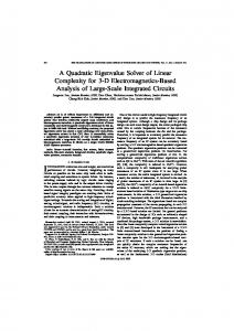
2.2 Mechanisms of Noise Generation The mechanisms of tire-road noise generation are stated to be extremely complex. They are commonly divided into two main groups according to the media in which they occur and their effects. The first one is related to the mechanical vibrations of the tire, termed “structure-borne”, and the second, related to the aerodynamic phenomena, called “air-borne”. The structure-borne noise can further be classified into impacts and shocks, and adhesion mechanisms [Nelson and Phillips 1994]. The relative contributions of these mechanisms vary with the type of tire, road surface, and vehicle speed [Sandberg and
12 Ejsmont 2002, Nelson 1994].
Figure 2.1 shows these mechanisms, and they are
described in the following sections.
Figure 2.1 Overview of noise generation mechanisms (After Nelson 1994)
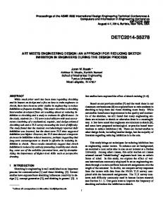
2.2.1 Structure-Borne Noise – Impacts and Shocks Vibrations are generated in the tires due to the impacts and deflections which occur as the tread blocks enter and leave the contact with the road surface and as a result of movement of tread elements in contact with the pavement. Vibrations in the tread and sidewall of the tire excite the air surrounding the tire, generating sound pressure waves that propagate away from the tire. Figure 2.2 is a concise representation of the mechanisms of tire-road noise generation, depicting the mechanisms as the tire rolls. As the tread block impacts the road surface, vibrations are driven radially into the tire. While the tread block moves through the contact patch, it is subjected to tension, whereas the tension is released when the block leaves the contact patch. This sudden release of tension returns the tire back to its undeflected rolling radius. This phenomenon is known as block snap-out, which
13 excites both the radial and tangential vibration modes [Nelson and Phillips 1994]. The tread compression, as shown in Figure 2.2, also induces radial vibration of the tire carcass. Both these phenomena occur at the lower end of the frequency range (1 KHz) [Bernhard 2002, BE 3415 1994].
Tire
Travel
Tire Vibration – Structure-borne
Travel
Tread block compression
Tread block Air pumping
Tire
Travel
Tire vibration
Horn Effect
Air-borne Air pumping Air pumping
Figure 2.2 Different mechanisms of tire-road noise generation
2.2.2 Structure Borne Noise – Adhesion Mechanisms Adhesion mechanisms are set up by the tire vibrations associated with the frictional losses created in the contact patch between the tire and the pavement [Sandberg
14 and Ejsmont 2002].
These are predominantly tangential forces, produced by the
changing radial deflection when the tire flattens in the contact patch. These forces are resisted by friction and tire stiffness. The friction mechanism is governed by the small scale roughness characteristics or microtexture of the pavement surface [Nelson 1994].
2.2.3 Air Borne Noise Tire-pavement noise is also generated by several mechanisms which are related to the movement of air in the cavities of the tread pattern. The most common of the airborne mechanisms is air pumping, shown in Figure 2.2. When the tread block enters the contact patch, air is sucked in between the grooves of the tread pattern, and when it leaves the contact patch, air is pumped out. The pressure modulations caused by this process is responsible for high frequency noise.
Additional air-borne generation
mechanisms include: (i)
Air turbulence, which is the turbulence around the tire due to the tire displacing air when rolling,
(ii)
Pipe resonance, which is the air displacement in the grooves in the tire tread, and
(iii)
Helmholtz resonance, which is the air displacement into or out of the connected air cavities in the tread pattern and pavement surface.
The latter two mechanisms are often considered as special cases of air pumping [Sandberg and Ejsmont 2002, Bernhard 2002].
15 2.2.4 Amplification or Reduction Mechanisms Though not strictly generation mechanisms, several other mechanisms in addition to the primary ones described earlier also have been found to augment or reduce the tirepavement interaction noise. The most important of them is the horn effect. Noise generated at or near the contact patch can be amplified due to the shape of the region between the tire and the pavement surface, immediately to the rear of the contact patch. Multiple reflections between the tire and pavement surface tend to occur, amplifying the sound [Descornet et al. 2000, Sandberg 2000, Nelson 1994, Bernhard 2002].
The
acoustic and mechanical impedance effects of the pavement surface are suggested as noise reducing mechanisms. The acoustic impedance depends on the communicating voids in the pavement whereas the mechanical impedance depends on the relative stiffnesses of the tire and the pavement.
2.3 Mechanisms of Noise Propagation Noise propagating from a sound source into free space attenuates with distance from the source, the rate of attenuation depending on the shape of the wavefront [Nelson 1994, Nelson and Phillips 1994]. If the source and receiver are close to the ground, reflections from the ground plane will occur. For a normal dense concrete pavement surface, the path difference between the directed and reflected wave is small and no destructive interference occurs between these waves at practical frequencies. Under these conditions, the sound waves arriving from both these paths add together to give a 6 dB increase over the free field amplitude.
The frequencies and amplitudes of these
16 interference effects depend greatly on the acoustic properties of the surface layer and the angle of incidence of the surface wave. When the surface layer is porous, the difference in path lengths between the direct and the reflected waves is large, and destructive interference occurs in the frequency range of 250 – 1000 Hz. The noise, as it reaches the observer, is of lower intensity in this case. This is one of the main advantages in using a porous pavement for noise abatement purposes.
2.4 Pavement Characteristics that Influence Noise It is widely recognized that the pavement surface has a very significant effect on the traffic noise. There are several pavement characteristics that are reported to influence the noise generated by tire-pavement interaction [Descornet et al. 2000, Sandberg and Ejsmont 2002].
2.4.1 Macrotexture This is defined as the deviation of a road surface from a true planar surface with the characteristic dimensions along the surface ranging from 0.5 mm to 50 mm. It is most often thought of as determined by the aggregate prominent on the surface. Macrotexture should have high amplitudes in the 0.5 to 10 mm wavelength and low amplitudes in the 10 to 50 mm wavelength to reduce tire noise [BE 3415 1994]. Treatments like grooving and grinding also create macrotexture [Descornet and Fuchs 1992, Descornet et al. 2000]. Surfaces are designed with sufficient macrotexture to
17 obtain suitable water drainage also, resulting in enhanced wet skid resistance. Mixture proportioning and surface finishing influence the macrotexture. Macrotexture is stated to have a very high influence on the noise generated [Sandberg and Ejsmont 2002, Nelson and Phillips 1994].
2.4.2 Megatexture Megatexture is defined as the deviation of a road surface from a true planar surface with the characteristic dimensions of 50 mm to 500 mm along the surface. It can be a defect in the pavement surface, resulting from the wear and fatigue of the surface material.
An inhomogeneity in macrotexture can also result in megatexture.
Megatexture exerts considerable influence on the noise generated, and should be minimized to reduce noise. Further, characteristic dimensions along the surface of 0.5 m to 50 m are sometimes termed as roughness, or unevenness.
2.4.3 Microtexture Microtexture is defined as the deviation of a road surface from a true planar surface with the characteristic dimensions along the surface of less than 5 mm. The influence of microtexture on noise is not as high as either macrotexture or megatexture. The ranges of texture and their most significant anticipated results are shown in Figure 2.3 [Wayson 1998].
18
Tire wear Rolling resistance Tire-road friction Exterior
tire-road noise
Noise in vehicles Discomfort and wear in vehicles Megatexture
Unevenness
50 m
5m
Microtexture
Macrotexture
50 mm
0.5 mm
Figure 2.3 Ranges of texture and their most significant anticipated results (after Wayson 1998). Unfavorable effects are shown in the shaded boxes
2.4.4 Porosity The significance of surface porosity in the noise propagation mechanism has been explained in Section 2.3. Porosity effectively reduces the air pumping effect, thereby reducing the tire noise [Bernhard 2002, Sandberg and Ejsmont 2002, BE 3415 1994]. The amplifying effect of the acoustic horn is also reduced when the sound waves are allowed to attenuate through the pores in the surface layer of the material. Acoustic absorption occurs when sound waves pass through the series of pores in the material. Details of the effect of porosity will be given later in this chapter.
19 2.4.5 Friction and Noise Friction is a property of the tire-road interaction that is derived from a number of tire and road surface characteristics. Due to friction, the tire may transmit longitudinal and lateral forces between the road and the vehicle. Friction constitutes a key factor for safety and drivability. It was believed that coarse (and hence noisy) surfaces were necessary in order to ensure good skid resistance. But it is now accepted that high friction and low noise are not conflicting requirements [PIARC 1991]. The road surface characteristics that determine friction are megatexture, macrotexture, microtexture, and the pavement interacting with the rubber of the tire. Megatexture and macrotexture can be measured directly but microtexture measurements are indirect, mainly from tire-road friction, using British Pendulum method [Sandberg and Ejsmont 2002]. The skid resistance of various types of road surfaces were calculated using sensormeasured texture depth (SMTD), obtained from laser profile devices [Phillips et al. 1994]. It was concluded from this study that high levels of SMTD implying good skid resistance are associated with high levels of megatexture, and therefore high levels of tire-road noise. For porous surfaces, which retain the texture in the form of pores, the skid resistance was found to be higher, even without high levels of megatexture.
2.5 Low Noise Concrete Pavements A “low noise” pavement is defined as one, which, when interacting with a rolling tire, influences vehicle noise in such a way as to cause at least 3 dB lower vehicle noise than obtained on conventional and most common road surfaces [Sandberg and Ejsmont 2002].
20 Descornet et al (2000) has stated three basic rules for designing a low noise pavement: (ii)
Sufficiently deep macrotexture (minimum 0.5 mm texture depth), using small to medium sized aggregates (< 10 mm),
(iii) Alternatively, the role of macrotexture can be played by porosity. Pores should be connected to the surface and should be interconnected (around 15% connected voids), and (iv) Minimize megatexture by ensuring that macrotexture is homogeneous. Sandberg and Ejsmont (2002) also recommend the above three methods to design low noise pavements, but add the following points: (i)
Avoid very smooth macrotextures, instead maximize macrotexture at wavelengths around 2-8 mm, and
(ii)
Construct the wearing course with as high a porosity that is viable from a durability standpoint and have wide channels to avoid pore clogging. Of several methods of making low noise concrete pavements, only non-porous
surfaces are discussed in this section. Porous concrete is dealt with in detail under a separate section.
2.5.1 Exposed Aggregate Concrete This technique consists of removing the top layer of paste / mortar either by mechanical means or chemical means (spraying retarding agent on fresh concrete surface), and exposing the aggregates to create a certain surface texture [Descornet et al. 2000, Descornet and Fuchs 1992, Descornet et al. 1993, Nelson and Phillips 1994, BE
21 3415 1994]. It has been found that exposing the aggregates can reduce noise levels only if the aggregate sizes are relatively small. The lower noise properties of these surfaces can be related to the relatively low levels of megatexture found for this surface. This is accomplished by using a longitudinal smoothing beam. Exposing the aggregates ensures adequate levels of macrotexture, and hence skid resistance and durability.
Exposed
aggregate concrete is sometimes called “whisper concrete”.
2.5.2 Chip Sprinkling The sprinkling treatment consists of spreading highly polish resistant aggregate chippings of a given size on the pavement surface under construction, and partly embedding them so as to create a rough surface macrotexture. The chippings used are in the size range of 10-15 mm. Due to the difficulty in uniformly embedding the chippings, this technique never went beyond the experimental stages [Descornet et al. 1993].
2.5.3 Tining or Grooving A rake with a number of tines is pulled on a fresh concrete surface to create grooves on the surface. This process is called tining. Three major types of tining are identified by the main direction of the surface texture – longitudinal, transverse, and random. The spacing of the tines can be uniform or random. Tines are typically 2-5 mm wide, 3-5 mm deep, and the spacing ranges from 10 to 40 mm. Grooving the hardened concrete also produces such texture. Random surface textures are generated either by grooving the surface at an angle, or by using different de-mortaring techniques. Grooves
22 typically are deeper and wider than the tines. It has been reported that road surfaces with longitudinal and random textures are less noisy than transversely textured surfaces [Wayson 1998, Kuemmel 2000]. The degree of noise reduction is determined by the characteristic distribution of macro- and megatexture on the surface. A pure longitudinal texture is often advisable since the tread will then ride on smooth and flat longitudinal ridges and not push down the parts of tire rubber into the groove each time a new groove is impacted. This reduces tire radial vibration, as well as air pumping. The potential disadvantages are that there are no escape channels for water during heavy rain, and trouble with steering of motorcycles.
2.5.4 Grinding Grinding is a special case of longitudinal texturing in which the concrete surface is ground using densely spaced diamond saw wheels. This process removes ridges and other uneven features and leaves a track of fine and densely spaced grooves in the treatment direction. Grinding is often used as a rehabilitation technique to pavement surfaces that have become rough and uneven, though it can be used for new surfaces as well. The level of smoothness that is obtained can be comparable to a new surface.
2.6 Porous Concrete (Enhanced Porosity Concrete - EPC) Concretes with higher than normal porosity and pore sizes, which enable water to drain through them quickly, are known as porous concretes, pervious concretes or Enhanced Porosity Concretes (EPC). The latter term will be used throughout this study.
23 They are typically produced by gap grading aggregates, eliminating / minimizing the use of sand, and using low binder contents. It has been reported that an EPC layer over a conventional concrete base is one of the efficient means of reducing pavement noise [BE 3415 1994, Christory et al. 1993, Descornet et al. 2000, Sandberg and Ejsmont 2002]. Though EPC was used in pedestrian areas and parking lots in Japan as early as 1983, its use in United States and Europe was not popular till the 1990s when the tirepavement interaction noise became a prominent issue. It was reported that EPC resulted in a 6 dB(A) (A-weighted average – Sandberg and Ejsmont 2002, Nelson 1994) reduction in noise level compared to the conventional pavement in a study in Belgium [Descornet et al. 2000]. A 5-6 dB(A) reduction was also reported by Nissoux et al. (1993).
2.6.1 Requirements for an Effective EPC Pavement For EPC to perform effectively with respect to its acoustic behavior, it has been recommended that 15-25% interconnected porosity is required [Christory et al. 1993, Nelson and Phillips 1994, Onstenk et al. 1993, BE 3415 1994, Descornet et al. 2000]. But it is also necessary that the material has adequate mechanical resistance and durability. A listing of the desirable properties has been given by Onstenk et al. (1993). (i)
Significant noise reduction and drainage properties,
(ii)
Acceptable strength and stiffness,
(iii) Adequate surface properties with respect to traffic safety – skid resistance, evenness, (iv) Sufficient service life – bonding to underlying dense concrete, freeze-thaw resistance, (v)
Construction by means of available techniques, and
24 (vi) Costs comparable to conventional pavements.
2.6.2 Advantages of EPC Pavements The advantages of using an EPC pavement in place of a conventional pavement are three-fold – (i) Ground water recharging, (ii) Reduced hydroplaning, and (iii) Noise reduction. The first two were the prominent reasons for using EPC before the tirepavement noise issues took center stage, and its efficiency in acoustic absorption ascertained. EPC was used in the design of foundations for pavement structures to provide continuous drainage necessary for extending the service life of these structures. EPC was also reported to be used on the runway of airports, primarily for its better drainage capacities. EPC pavements also exhibited reduced hydroplaning [Christory et al. 1993].
2.7 Materials, Mixture Proportioning, and Construction Procedure of EPC Pavements In order to achieve such desirable properties with high porosity, materials and mixture proportioning method should be chosen taking into account a host of factors. Those parameters are described as follows.
2.7.1 Aggregate Sizes and Gradation To ensure that EPC contains about 15-25% open porosity, careful selection and gradation of aggregates are necessary.
Gap-graded aggregates, resulting in lack of
material to fill out the space between the larger aggregates, are the most favored choice.
25 The accessible porosity and strength are reported to be a function of the grain size of the fine aggregate in relation to that of the coarse aggregate [BE 3415 1994]. The maximum grain size of coarse aggregate has to be limited to 10 mm as per another study [Onstenk et al. 1993]. This study also reports that the grain size of fine aggregate has a major effect on accessible porosity and strength, while the grain size of coarse aggregate does not have a major effect. Gerharz (1999) recommends that the aggregate size for EPC has to be between 4 and 8 mm. The use of coarse aggregates of size up to 30 mm and sand of size less than 2.5 mm has been reported [Jing and Guoliang 2002]. The use of larger aggregate sizes (20 mm maximum size) has been recommended for EPC since they result in large sized pathways in the material, thereby preventing clogging [Nelson 1994]. Recently, ACI Committee 522 (2003) has suggested that the aggregate sizes for EPC should be between 19 mm and 9.5 mm.
2.7.2 Cement Content EPC is proportioned with just enough cement content required to bind the aggregates together. This is to minimize the occurrence of excess cement paste seeping through the material structure, reducing its openness. The water-binder ratio also is kept low for the same reasons. It is recommended to conduct binder drainage tests to ascertain the optimum binder content for the aggregate gradation chosen [Nelson 1994]. This procedure is expected to ensure high residual porosity, with acceptable strength characteristics.
26 2.7.3 Additives The use of silica fume (10% by weight of cement), and a superplasticizer were reported not to increase the strength of EPC [Onstenk et al. 1993]. Polymer additives were reported to result in an increase in strength as well as freeze-thaw resistance of EPC. Since the cement content of EPC is low, fine mineral admixtures and organic intensifier (polymer) were incorporated in concrete to improve the microstructure and strength of EPC [Jing and Guoliang 2002].
2.7.4 Construction Procedure From a construction point of view, two alternatives are stated in literature for EPC – (i) wet on wet, and (ii) wet on dry [BE 3415 1994]. The “wet-on-wet” process consists of laying the conventional concrete base layer and the EPC top layer within a short time so that the base layer has not begun to set when laying the top layer. The benefit of this system is that no additional products are required to bond the two layers. In some cases, a retarding admixture is applied to the base layer so that it does not set before the EPC layer is placed. This process requires careful planning of the construction process – either two pavers, or modified pavers which can simultaneously lay two layers of different materials, are needed. It also necessitates the use of two mixing plants with different capacities, due to the different thicknesses used in both layers. The “wet-on-dry” process consists of laying the EPC layer once the conventional concrete in the base layer has hardened enough to sustain a roller on it. The bond between the two layers is obtained through the use of an adherent material which can be
27 cement based or polymer based. This may result in an increased cost. Moreover, the joints in the lower layer need to be sawed, and sealed to avoid cement paste from the top layer penetrating into it.
2.8 Mechanical Properties and Durability Characteristics This section describes the different mechanical properties and durability characteristics of EPC as described by various authors.
2.8.1 Compressive and Flexural Strengths The strength of EPC depends on the grain size distribution, accessible porosity, and the type and amount of additive used. A maximum compressive strength of about 18 MPa, at an accessible porosity of 25% has been reported. The maximum flexural tensile strength at this porosity was found to be about 4 MPa. Increase in tensile strength was observed when a polymer additive was used [Onstenk et al. 1993]. Flexural tensile strength of about 3 MPa was achieved for a total porosity of 25%, using 6-10 mm aggregates [Nissoux et al. 1993]. A 28-day compressive strength of 20 MPa, and flexural strength of 3 MPa has been reported for an EPC with 25% porosity in another study [BE 3415 1994]. Increase in aggregate size resulted in a reduced compressive strength, where as the addition of polymer and mineral admixture resulted in an increased strength [Jing and Guoliang 2002].
28 2.8.2 Water Permeation The water permeation capacity or the drainage properties are closely related to the accessible porosity. For an accessible porosity of 20-29%, the coefficient of permeability is about 0.01 m/s [BE 3415 1994]. It has also been found from this study that the fine aggregate determines the permeability. A permeability of around 36 l/s/m2 has been reported for EPC in another study [Nissoux et al. 1993].
2.8.3 Durability Characteristics Since EPC forms the top layer of the pavement, it is exposed to the most severe conditions. Some studies have suggested that a polymer additive is required to develop sufficient freeze-thaw resistance in EPC [BE 3415 1994, Gerharz 1999, Onstenk et al. 1993], whereas results of field implementation of EPC in low volume pavements show that EPC proportioned with gap graded aggregates and with a porosity of around 20% sustained freeze-thaw cycles without any additives [GCPA 2003]. Freeze-thaw tests have also been conducted by submerging the lower part of EPC in 3% NaCl solution. This type of testing is reported to be more severe than the conventional freeze and thaw tests [Onstenk et al. 1993].
2.9 Acoustic Absorption of EPC Several studies on the acoustic absorption of EPC have concluded that the porosity accessible to the sound waves, and the thickness of the porous layer are the significant factors that determine the acoustic absorption of EPC [Nelson 1994, Francois
29 and Michel 1993, Onstenk et al. 1993, BE 3415 1994, Descornet et al. 1993]. The frequencies and amplitudes of the maxima and minima of the absorption coefficients are related to the porosity of the surface layer, air flow resistance, tortuosity of the pore network, and the thickness of the porous layer [Descornet et al. 2000]. Varying the thickness affects the frequency at which the maximum acoustic absorption occurs while increasing the porosity is said to be beneficial in increasing the absorption at any frequency. The first absorption peak determines the effectiveness of the material in terms of noise reduction. The optimization of acoustic properties of EPC therefore depends on the efficiency in obtaining the maximum amplitude and width of the first peak, which in turn depends on the four above-mentioned parameters.
However, from a practical
standpoint, only the porosity and thickness can be designed and achieved by proper mixture proportioning whereas the tortuosity and flow resistivity can be determined later only. Normal variations in air flow resistivity and tortuosity of the pore channels are reported to have only a marginal effect in the acoustic absorption of EPC [Nelson 1994]. A layer thickness of between 0.05 m and 0.08 m was arrived at as the optimum thickness to reduce tire-pavement noise, from this study.
To ensure significant acoustical
effectiveness (3 dB(A) reduction as compared to a dense surface), porous surfaces are reported to require a minimum voids content of 20%, and a minimum thickness of 40 mm [Descornet et al. 2000]. It has been stated in this study that the maximum acoustic absorption coefficient (α) measured using a standing wave tube on cores of 100 mm diameter should satisfy those given in Table 2.1. In a German study, an EPC pavement of 80 mm thickness and 25% porosity exhibited an average noise reduction of about 6 dB(A) [Descornet et al. 2000].
30 Table 2.1 Maximum acoustic absorption coefficient measured from cores, for different frequencies (Italian specifications, Descornet et al. 2000) Frequency (Hz)
Acoustic absorption coefficient (α)
400-630
≥ 0.15
800-1600
≥ 0.30
2000-2500
≥ 0.30
2.10 Noise Reduction Mechanisms in EPC The primary mechanism with which EPC reduces the tire-pavement interaction noise is acoustic absorption. The component of noise that is eliminated by absorption is mainly the air-borne ones. However, there are several other mechanisms by which EPC reduce noise [Sandberg and Ejsmont 2002, Nelson and Phillips 1994, Descornet et al. 2000]. They are briefly described in this section. (i)
The open porosity prevents the development of high pressure gradients at the edges of the tire-road contact patch, and also within the contact patch. This is responsible for the reduction or even elimination of all air displacement noise generation mechanisms
(ii)
Small chippings in the surface results in the impact mechanism being not a very dominant effect
(iii) The porosity in the EPC results in acoustic absorption so that sound waves are dissipated into heat in the small pores inside the material. The acoustic absorption effect will influence not only the tire-pavement noise but also other types of vehicle noise
31 (iv) If sound is reflected between the pavement surface and the underbody of the vehicle a number of times, each reflection causes loss of acoustic energy (v)
The acoustically “soft” EPC surface will affect the acoustical impedance in and around the tire-road contact patch, as well as between the source and receiver. This is similar to the explanation of Section 2.3. The absence of a reflecting plane eliminates the horn effect.
2.11 Maintenance of EPC Pavements Concrete pavements are fairly durable and needs little maintenance as long as it is well designed and built. But the high amounts of porosity in EPC gives rise to certain special problems such as clogging of voids, bond between EPC and dense concrete, and freezing and thawing damages in cold climates [BE 3415 1994]. Studies have shown that a well designed and constructed EPC may not undergo freezing and thawing damage provided it is well draining. Clogging of pores is a serious issue which limits the draining capacity of EPC pavements and thus affects its freeze-thaw resistance. Clogging can occur because of depositions of dirt or dust from the surroundings, and wear products from the pavement and tire, in the voids of EPC. Also, the surface becomes somewhat compacted, and compaction occurs at the expense of the voids.
Many cleaning
methodologies have been recommended in the literature [Sandberg and Ejsmont 2002], but the most efficient one has been a combination of water jet blasting, dirt water suction, and vibrations transmitted by a “plane of water” between the water blasting and suction. An interesting method of “self cleaning” of porous pavements has been reported by the above authors. It is postulated that the most effective cleaning process is one that
32 takes place during heavy rainfall and when vehicles travel at high speed on the pavement. The removal of water at the leading edge of the tire-road interface, and the suction of dirt water from the trailing edge may occur with very high pressure gradients, giving an efficient self-cleaning effect. For instance, at a vehicle speed of 90 km/h, the tire moves at 25 mm per millisecond. This indicates that the pressure at a particular spot changes from atmospheric pressure to a large value in just a millisecond. This is equivalent to shooting a “water-bomb” on the surface.
2.12 Summary This first part of this chapter has dealt with tire-pavement interaction noise. The mechanisms of generation, amplification, and propagation have been discussed. The pavement characteristics that have a bearing on these mechanisms, and the various low noise concrete pavement types are elaborated. In the latter part of the chapter, an extensive review on materials and manufacturing methods, physical and mechanical properties, durability characteristics of Enhanced Porosity Concrete is provided.
33
CHAPTER 3: MATERIALS, MIXTURE PROPORTIONING, AND TEST METHODS
3.1 Introduction This chapter explains the materials used in this study, mixture proportions adopted, and the test methods employed to study the various properties of Enhanced Porosity Concrete (EPC). Existing testing methodologies reported in standards were adopted to study some of the properties of EPC, whereas custom test equipment and procedures were developed to ascertain some other properties. Detailed descriptions of the experimental set up developed, and the testing method are provided.
3.2 Materials This section gives an outline about the various materials used in the experimental investigations. The materials are kept constant throughout the study so as to nullify the influence of change in materials on the physical, mechanical, and durability characteristics of EPC.
34 3.2.1 Cement Commercially available Type I Ordinary Portland Cement manufactured by Lonestar Industries was used for the entire study. Table 3.1 summarizes the chemical properties of the cement. Table 3.1 Chemical properties of cement C3S (%) -62.0
C3A (%) 15.0 (max) 9.0
Total
Insoluble
Loss on
MgO
SO3
Alkali (%)
Residue (%)
Ignition (%)
(%)
(%)
--
0.8 (max)
3.0 (max)
0.5
1.94
0.58
6.0 (max) 1.82
4.5 (max) 2.67
3.2.2 Fine Aggregate The fine aggregate used for the study was a locally available river sand, with a water absorption of 2.3%. The sand conforms to ASTM C 128-94.
3.2.3 Coarse Aggregate Limestone aggregates were used as coarse aggregates in this study. Aggregates were sieved into different size fractions to create gap grading used in this study. The aggregate sizes used were: # 8 (passing 4.75 mm and retained on 2.36 mm sieve), # 4 (passing 9.5 mm and retained on 4.75 mm sieve), and 3/8” (passing 12.5 mm and retained on 9.75 mm sieve).
35 3.2.4 Silica Fume A commercially available silica fume was used in some of the mixtures investigated to ascertain its impact on the mechanical and acoustical properties. Addition of silica fume was carried out at 6% and 12% by weight of cement.
3.2.5 Fibers To prepare fiber reinforced EPC, Polypropylene fibers, 50 mm long and 1-2 mm wide were used. The fibers had a density of 910 kg/m3.
3.3 Mixture Proportioning and Specimen Preparation This section describes the mixture proportions used in this study, mixing procedure and the method of preparing specimens for the various testing that are described later.
3.3.1 Mixture Proportions The water-cement (w/c) ratio used for all the mixtures investigated in this study was kept constant at 0.33. The cement content was established by providing just enough paste to coat the aggregates since an excessive amount of paste may drain through the pores of the material. It was found out from a trial and error process that the aggregatecement ratio could be kept around 5.6 at the selected w/c to achieve this. The mixtures were prepared with either the single sized aggregates alone as explained in Section 3.2.3, or binary blends of these mixtures. Blends were prepared by replacing 25, 50, and 75%
36 by weight of the larger sized aggregates successively by smaller sized aggregates. To study the influence of sand, # 4 aggregates were replaced by 2.5, 5.0, and 7.5% by weight of natural sand. Silica fume was added to the mixtures at 6% and 12% by weight of cement to study its influence on the properties of EPC. Table 4.2 shows the mixture proportions used in this study.
#8 Aggregate (2.36-4.75mm)
Fine Aggregate (Sand)
%
%
%
Silica Fume Addition by Cement Weight
#4 Aggregate (4.75-9.5mm)
%
Water-to-Cement Ratio
3/8" Aggregate (9.5-12.5mm)
Mixture I.D.
Table 4.2 Proportions of EPC mixtures used in this study
%
Gap grading and Single Sized Aggregate Size PC-100-3/8 PC-100-#4 PC-100-#8
100 0 0
0 100 0
0 0 100
0 0 0
0.33 0.33 0.33
0 0 0
0 0 0 0 0
0.33 0.33 0.33 0.33 0.33
0 0 0 0 0
0 0 0 0 0
0.33 0.33 0.33 0.33 0.33
0 0 0 0 0
0 0 0
0.33 0.33 0.33
0 0 0
0 2.5 5.0 7.5
0.33 0.33 0.33 0.33
0 0 0 0
0 0 0
0.33 0.33 0.33
0 6 12
Blending # 8 and # 4 Aggregates PC-100-#8 PC-75-#8, 25-#4 PC-50-#8, 50 #4 PC-25-#8, 75-#4 PC-100-#4
0 0 0 0 0
0 25 50 75 100
100 75 50 25 0
Blending # 8 and # 3/8" Aggregates PC-100-#8 PC-75-#8, 25-3/8 PC-50-#8, 50-3/8 PC-25-#8, 75-3/8 PC-100-3/8
0 25 50 75 100
0 0 0 0 0
100 75 50 25 0
Blending # 4 and # 3/8" Aggregates PC-100-#4 PC-50-#4, 50-3/8 PC-100-3/8
0 50 100
100 50 0
0 0 0
Addition of Sand PC-100-#4 PC-95-#4, 5-Sand PC-97.5-#4, 2.5-Sand PC-92.5-#4, 7.5-Sand
0 0 0 0
100 97 95 92
0 0 0 0
Addition of Silica Fume PC-100-#4 PC-100-#4, 6-SF PC-100-#4-12-SF
0 0 0
100 100 100
0 0 0
37 3.3.2 Mixing and Placing Procedure The constituent materials were batched immediately prior to mixing.
The
weighed quantity of aggregates was added to the mixer, followed by cement, and silica fume, if desired. For mixtures that incorporated fibers, they were slowly added at this stage. Water was slowly added while the dry materials were being mixed in a pan mixer. The mixer was allowed to run for three minutes. At the end of three minutes, the bottom and sides of the mixer were scrapped, and the mixer was allowed to rest for three minutes. A final two minutes of mixing followed this step. The contents of the mixer were then discharged from the mixing pan into the molds using scoops. The concrete was placed in the forms in two equal lifts. The forms were vibrated on a table vibrator while the concrete was being placed. In addition, the sides of the forms were struck with rubber mallet so as to ensure that the molds are properly filled. No needle vibrator was used since the workability of EPC is low because of gap graded aggregates and low cement content. The forms were finished and were kept under wet burlap for the first 24 hours. After this period, the specimens were removed from the molds, and were kept in the moist room at a relative humidity of greater than 98% till further testing.
3.4 Test Procedures The following section gives an outline of the various test procedures employed in this study to obtain the material properties of EPC.
38 3.4.1 Flexural Strength Determination Flexural strength was determined in accordance with ASTM C 78-02. Two tests were conducted on each mixture from a single beam (150 mm x 150 mm x 700 mm), and the average strength reported. Figure 3.1 shows the loading arrangement for flexural strength testing. The first flexural strength test was conducted on 450 mm span of the beam and the second test on the longer remaining portion of the beam after the first flexural failure.
Load
Span 1
Load
Span 2 Figure 3.1 Flexural strength determination
3.4.2 Porosity Determination using Image Analysis Porosity was determined using cores of 95 mm diameter and 150 mm length, drilled from the 150 mm x 150 mm x 700 mm beam specimens. The sides and the bottom of the core was sealed using a tape, leaving the top surface open. The core was then placed in a 100 mm x 200 mm plastic cylindrical mold and flooded with a low viscosity epoxy. Approximately 25 mm of excess epoxy was left above the top of the specimen. The mold and the specimen was then externally vibrated using a vibrating
39 table for eight to ten minutes to allow the epoxy to permeate into all accessible pores. The specimen was left undisturbed for 24 hours allowing the epoxy to harden. After the epoxy hardened, the mold was stripped and the specimen was cut at depths of 12.5 mm, 37.5 mm, 62.5 mm, 87.5 mm, and 112.5 mm from the top surface, as shown in Figure 3.2. The epoxy impregnated slices were allowed to cure for twenty-four hours.
No
measurements were conducted on the bottom most slice. The bottom sides of each slice were then brushed clean to remove any debris left from the sawing.
Figure 3.2 Sectioning the core for image analysis The slices were then placed directly on a flatbed scanner over a clear plastic film, scanned in the grayscale mode, and a bitmap image created. Figure 3.3 shows the image processing procedure.
After capture, the images of each slice were cropped using
Microsoft Photo Editor® to create a smooth outer circumference with no edge effects and a uniform diameter of 69 mm (Figure 3.3 (a)). The light gray areas of this image correspond to the aggregates and paste whereas the dark areas correspond to both epoxyfilled and unfilled pores. The cropped images were then analyzed using ImagePro®
40 software.
A filter was used to “clean” the image by comparing each pixel to the
surrounding pixels, thereby removing miscellaneous marks that may otherwise interfere in the calculation of porosity. A mask was then applied to each image to darken the aggregates and paste, leaving the open and epoxy filled pores as bright objects (Figure 3.3 (b)). The area of the “bright objects” was computed in pixels (72641 white pixels), and the total porosity was calculated based on the known area of the pores and the known total area of the image (237463 pixels). After the initial grayscale image was obtained, the same specimen surface (scanned as a grayscale image) was then stained black using a fat-tip marker and scanned in the true color mode. This created a second image where the epoxy, aggregate, and paste could be segmented from unfilled pores (inaccessible pores), as shown in Figure 3.3 (c). The same image analysis procedure that was used on the initial grayscale images was applied to the true color bitmap of the stained slices; however, for the second image, the pore areas were masked dark and the flat surfaces of the plane bright (Figure 3.3 (d)). Again, the filter was used to clean the image and the area of the bright objects was computed in pixels. This allowed the area of the aggregate, paste, and epoxy filled pores to be determined (225087 pixels). The inaccessible porosity was then calculated by subtracting this value from the known total area of the image. Once the image analyses has been completed for each grayscale image and each true color image, the accessible porosities of each slice could be approximated by subtracting the inaccessible porosity (obtained from the stained slices) from the total porosity (obtained from the unstained slices). The averages of the values obtained from the slices were reported.
41
(a) Scanned image cropped to a diameter of 69 mm
(b) Image threshold established and cleaned white pixels (total porosity) counted
(c) Surface colored and rescanned, cropped to a diameter of 69 mm
(d) Image threshold established and cleaned black pixels (inaccessible porosity) counted
Figure 3.3 Image processing procedure
3.4.3 Porosity Determination using Volume Method Because of the presence of large interconnected pores in the EPC system, the following procedure was adopted to determine the volume porosity. The cylindrical specimens (95 mm in diameter and 150 mm long) that were cored from beams were
42 immersed in water for 24 hours to saturate the pores in the matrix. After this period, the sample was removed from water and allowed to achieve SSD condition. The sample was then enclosed in a latex membrane and the bottom of the cylinder was sealed using a stainless steel plate with silicone sealant. The mass of the sample, latex membrane, and the steel plate (M1) was measured. Water was added to the top of the sample until it was filled, which indicated that all the interconnected pores were saturated. The mass of the system filled with water was taken (M2). The difference in the mass ∆M = (M2-M1) represents the water in the pores. This mass was converted into a volume, expressed as a percentage of the total volume of the specimen to provide an indication of the total porosity.
3.4.4 Pore Size Determination The pore size was estimated using the grayscale images from the porosity measurements.
Measurements were conducted on middle three slices from each
specimen (Figure 3.2). As was done for porosity determination, the images were masked and filtered, leaving the pores as bright objects. The maximum and minimum diameters of the each of the selected pores were recorded. Since the pores are of varying sizes, and the process of establishing threshold intensity is likely to merge two very small bright features into one big feature and identify it as a pore, the average pore size thus obtained was not thought to be an adequate indicator of the representative pore sizes in the specimen.
The median of all the pore sizes greater than 1mm was chosen as an
approximation of the representative pore size of the sample, and is termed as the
43 “characteristic” pore size. The 1mm threshold was adopted to account for the fact that the imaging process records a large number of features of size less than 1mm and considering them in the analysis will always result in a median size that does not correlate to the physical sizes present in the system. However, pore sizes determined by this method are only estimates to provide an indicator of the sizes of the pores in the system and provide a useful method of comparison of different systems with varying aggregate sizes and blends.
3.4.5 Determination of Hydraulic Conductivity Since the EPC has a large interconnected pore network, the conventional methods that are used to evaluate the hydraulic conductivity of normal concrete are not directly applicable. To estimate the hydraulic conductivity of EPC, a falling head permeability cell has been designed, as shown in Figure 3.4. The permeability cell consists of a 250 mm long acrylic tube with an inner diameter of 92 mm. The top 150 mm of the tube was machined to an inner diameter of 95 mm so that the specimen can be seated on an O-ring at a distance of 100 mm from the bottom. A 50 mm diameter valve connects the bottom part of the tube to a vertical pipe through which water can drain out. The top of this pipe is positioned 10 mm above the top of the specimen so that no unsaturated flow occurs during the test. A graduated acrylic cylinder of 300 mm length was attached to the top of the specimen assembly and clamped tightly using a rubber sleeve. This was used to monitor the water level during the test.
44 95 mm
300 mm
Graduated cylinder
Drain pipe
150 mm
Top of the sample
10 mm
Sample
100 mm
O-Ring Valve
Figure 3.4 Test Set up to measure hydraulic conductivity The specimen was enclosed in a latex membrane (as was done for the electrical property measurements), and was inserted into the test set up. Water was added to the graduated cylinder to fill the specimen cell and the draining pipe. The specimen was preconditioned by allowing water to drain out through the pipe until the level in the graduated cylinder was the same as the top of the drain pipe. This eliminated any air pockets in the specimen and ensured that the specimen was completely saturated. With the valve closed, the graduated cylinder was filled with water. The valve was then open, and the time in seconds (t) required for water to fall from an initial head of 290 mm (h1)
45 to a final head of 70 mm (h2) noted. This procedure was repeated three times, and the average value of t was used. The coefficient of permeability (K) was calculated according to Darcy’s law as: K=
h A1l log 2 A2 t h1
3.1
where A1 and A2 are the areas of the cross-section of the sample and the tube respectively and l is the length of the specimen. For a given specimen geometry, and same initial and final heads, the coefficient of permeability is given as:
K=
A t
3.2
where A is a constant, which in this study was 0.084 m.
3.4.6 Measurement of Acoustic Absorption To evaluate the acoustic absorption characteristics of EPC, a Brüel & Kjær™ impedance tube was employed, as shown in Figure 3.5. Cylindrical specimens with a diameter of 95 mm were cored from beams after they were tested in flexure. Three specimen lengths – 150 mm, 75 mm and 37.5 mm were tested using the impedance tube. The sample was placed inside a thin cylindrical Teflon sleeve, into which it fits snuggly. The sample assembly was placed against a rigid backing at one end of the impedance tube which is equipped with a sound source. A plane acoustic wave generated by the sound source was propagated along the axis of the tube. Microphones placed along the axis of the tube were used to detect the sound wave pressure transmitted to the sample and the portion of the wave that is reflected (ASTM E-1050). The pressure reflection
46 coefficient (R) is the ratio of the pressure of reflected wave to that of incoming wave, at a particular frequency, expressed as:
e jkd1 − e jkd 2 P R = − jkd 2 e P − e − jkd1
3.3
where d1 and d2 are the distances from the specimen surface to the closest and farthest active microphones respectively, j is an imaginary number ( − 1 ), k is the wave number (ratio of angular frequency to the wave speed in the medium) and P is the ratio of acoustic pressures at the two active microphone locations.
Active Microphones d2 d1
Sound Source Sample Location
Figure 3.5 Impedance tube set up A data acquisition system (PULSE ™) is attached to the impedance tube, which converts the signals in the time domain to one in the frequency domain. A software program written in Matlab™ allows graphic display of the real and imaginary
47 components of the impedance with respect to the frequency. The program has also been tailored to output the variation of acoustic absorption coefficient with frequency. The absorption coefficient (α) is commonly reported as a measure of a material’s ability to absorb sound. A material with an absorption coefficient of 1.0 indicates a purely absorbing material whereas a material with an absorption coefficient of 0 indicates that it is purely reflective. The absorption coefficient at each frequency can be calculated from the pressure reflection coefficient (R) as given in Equation 4.4.
α = 1-|R|2
3.4
In this work the frequency range of interest was limited from 100 Hz to 1600 Hz. A threshold of 100 Hz was established because at very low frequencies, the acoustic pressures were difficult to stabilize. Frequencies higher than 1600 Hz could be measured accurately only when the impedance tube has a small diameter. (To achieve acoustic measurements over the widest range of frequencies, and to ensure that a “standing wave” is generated inside the impedance tube, its diameter should be as small as possible). Preparation of homogeneous concrete samples of such small sizes tends to be difficult due to the size of the aggregates.
3.4.7 Electrical Impedance Spectroscopy Electrical Impedance Spectroscopy (EIS) was used to determine the bulk resistance of EPC samples, in order to estimate the conductivities. EIS measurements were conducted in this study using a Solartron 1260 ™ Impedance / Gain-Phase analyzer that was interfaced with a personal computer for data acquisition. A typical Nyquist plot
48 (plot of real versus imaginary impedance) obtained from EIS measurements consists of two arcs – the bulk arc and the electrode arc. The two arcs meet at a point where the imaginary component of the impedance is minimum, and the corresponding real impedance is the bulk resistance (Rb) of the sample. Figure 3.6 shows the specimen set up that was used for the EIS experiments. The cylindrical EPC specimen, 95 mm in diameter, and 150 mm long was enclosed in a latex membrane to contain the electrolyte. The bottom of the specimen was sealed to a stainless steel plate using silicone sealant.
The specimen was saturated with the
electrolyte and another stainless steel plate with a small acrylic dyke was placed at the top of the specimen, with a piece of porous foam in between. The entire set up was firmly gripped with adjustable clamping mechanism. The stainless steel plates served as the electrodes and alligator plugs from the impedance analyzer were attached to the electrodes. The impedance measurements were made over the frequency range of 1 MHz to 10 Hz using a 250 mV AC signal. Using the bulk resistance (Rb) obtained from the Nyquist plots, the effective electrical conductivity (σeff) of the sample was calculated as:
σ eff =
l Rb A
3.5
where l is the specimen length and A is the cross sectional area of the specimen. The electrolytes used in this study were sodium chloride (NaCl) solutions of varying concentrations (1%, 3%, and 10%). The conductivity of 1% NaCl solution was 1.56 S/m whereas the conductivities of 3% and 10% solutions were 4.40 S/m and 12.40 S/m respectively.
49
C-clamp to hold the specimen in place Stainless steel plate top electrode with dyke
Specimen enclosed in latex membrane
Stainless steel plate as bottom electrode
Figure 3.5 Specimen set up for EIS experiments
3.4.8 Dynamic Modulus of Elasticity The dynamic modulus of elasticity was determined using Grindosonic ™ equipment, as per ASTM E 1876-01. The specimen was supported on rollers at a distance of 0.224L from the edges (L is the specimen length). The pick up of the Grindosonic equipment was positioned on the center of the side face of the specimen and a light impact was given on the center of the top face of the specimen to transmit flexural waves through the specimen.
The instrument indicated the fundamental flexural
frequency. The procedure was repeated for 5 times (a very consistent reading was obtained in this case) and the average was taken as the fundamental flexural frequency of the specimen. The dynamic modulus of elasticity is given by:
50
L3 E = 0.9465mf 3 T1 t b 2 f
3.6
where E is the dynamic modulus of elasticity in Pa, m is the mass of the specimen in g, ff is the fundamental flexural frequency of the specimen in Hz, L is the specimen length in mm, t and b are the specimen thickness and width respectively in mm, and T1 is a correction factor to account for the finite length of the bar, Poisson’s ratio and so forth. The equation for calculation of T1 is given in ASTM E 1876.
3.4.9 Freezing and Thawing Freezing and thawing studies on EPC were carried out using two methods: (i) rapid freezing and thawing in water, as per ASTM C 666 Procedure A, and (ii) slow freezing and thawing in water, in a controlled temperature chamber where the specimens are subjected to one freeze-thaw cycle per day. The temperature of the slow freezing and thawing chamber cycled from -16 0C to 22 0C. The fundamental flexural resonant frequencies of the specimens were determined prior to freezing, and then periodically during the test. A waveform spectrum analyzer was used to determine the frequencies. The relative dynamic modulus (Pc) was calculated according to Equation 3.7 periodically during the test. n2 Pc = 12 × 100% n
3.7
where n1 is the fundamental frequency after a certain specified number of cycles, and n is the fundamental frequency before freezing and thawing cycles were started.
51
CHAPTER 4: PROPERTIES AND PORE STRUCTURE FEATURES OF EPC
4.1 General This chapter deals with the fundamental mechanical properties (flexural strength), and pore structure features (porosity, pore size, and permeability) of EPC. The influence of aggregate size and gradation on the pore structure features and the mechanical properties are presented. In addition, the variation in mechanical properties with pore structure features, as well as with addition of fibers, is explained. The central idea of this chapter therefore is to bring out the significant features of the pore structure of EPC and develop an understanding of how it affects the other properties.
4.2 Aggregate Sizes and Pore Sizes The three sizes of aggregates used to produce gap graded EPC mixtures in this study were # 8 (passing 4.75 mm and retained on 2.36 mm sieve), # 4 (passing 9.5 mm and retained on 4.75 mm sieve), and 3/8” (passing 12.5 mm and retained on 9.75 mm sieve). Moreover, binary blends of these aggregate sizes were also used as given in Table 3.2. The pore sizes are significantly influenced by the aggregate sizes and their gradation. This section discusses the influence of single sized aggregates as well as aggregate blends on the pore sizes of various EPC mixtures.
52 4.2.1 Influence of Single Sized Aggregates on Pore Size The plot of aggregate size versus characteristic pore size shown in Figure 4.1 for EPC mixtures with single sized aggregates.
Characteristic pore size (mm)
6
Dp = 1.44 + 0.36*Dagg R2 = 0.93 4
2
#8 #4 3/8"
0 0
2
4
6
Aggregate size (mm)
8
10
Figure 4.1 Variation of characteristic pore size with aggregate size for single sized aggregate EPC mixtures The mixture made using only 3/8” aggregates has the largest characteristic pore size (4.76 mm) among all the mixtures investigated whereas the mixture with only # 8 aggregates has the smallest pore size (2.17 mm). An increase in aggregate size therefore is found to result in an increase in characteristic pore size. The relationship between the aggregate size and the characteristic pore size for a single sized aggregate EPC mixture can be described using the linear equation given below: Dp = 1.44 + 0.36 Dagg
4.1
where Dp is the characteristic pore size, and Dagg is the aggregate size, both in mm.
53 4.2.2 Influence of Aggregate Blends on Pore Size The variations in characteristic pore size with aggregate blends are shown in Figures 4.2 and 4.3. The characteristic pore size is plotted against the percentage of larger aggregates replacing the smaller ones. Figure 4.2 shows the relationship between the aggregate size and pore size for an aggregate size ratio of 2.0 in the blend (i.e, 3/8” aggregates replacing #4, and # 4 replacing # 8), where as Figure 4.3 depicts the relationship for an aggregate size ratio of 4.0 (i.e, 3/8” replacing # 8).
Characteristic pore size (mm)
6 3/8" replacing #4 #4 replacing #8
5
Aggregate size ratio: 2.0 4
3
2 0
20 40 60 80 Percentage of bigger aggregates replacing smaller ones
100
Figure 4.2 Variation of characteristic pore size with aggregate size for binary blends with aggregate size ratio of 2.0 It can be readily noticed that replacing the smaller sized aggregates with an increasing percentage of larger sized ones increases the characteristic pore size. This happens because the introduced coarser particle may not be able to fit in the void left
54 behind by the removed finer particle. Also, according to the theory of particle packing, when fewer coarser particles are introduced in a mixture of finer particles, there is a further amount of voids introduced in the packing of finer particles at the interface, called the wall effect.
Characteristic pore size (mm)
6 3/8" replacing #8 5
Aggregate size ratio: 4.0
4
3
2 0
20
40
60
80
Percentage of bigger aggregates replacing smaller ones
100
Figure 4.3 Variation of characteristic pore size with aggregate size for binary blends with aggregate size ratio of 4.0 The plots are essentially parallel when the aggregate size ratio is 2.0, (combination of either # 4 and # 8 or # 4 and 3/8”), as seen in Figure 4.2. The variation is steepest when the smallest size is replaced by the largest size (i.e., # 8 by 3/8” aggregates, giving an aggregate size ratio of 4.0), as depicted in Figure 4.3. Figures 4.2 and 4.3 show the dependence of pore size on the ratio of aggregate sizes. The trends indicate that an increase in aggregate size, be it in single sized, or blended system, increases the characteristic pore size of the system.
55 The characteristic pore size is an important parameter in the design of EPC for optimal acoustic characteristics as well as hydraulic permeability, as will be explained later. Figures 4.1, 4.2 and 4.3 can also be used as design aids in such circumstances. Based on the required characteristic pore size, which is dictated by the requirements of acoustics or permeability, the optimal aggregate size (in the case of single sized aggregates) or the proportion of different aggregate sizes (in the case of blends) can be obtained from these figures.
4.3 Aggregate Sizes and Porosity The aggregate sizes and gradation have a significant effect on porosity of EPC mixtures. This section explains how the aggregate sizes and gradation influences the porosity of EPC mixtures. As explained earlier, porosity was determined using an image analysis procedure as well as a volumetric procedure. The figures in this section uses data from the image analysis procedure, and as a means of comparison between porosities obtained from both the methods, a Table is included later in this section. Figure 4.4 illustrates the variation in accessible porosity with percentage of # 8 aggregates, the remaining percentage made up of either # 4 or 3/8” aggregates, i.e., 50% # 8 aggregates indicate that the remaining 50% is made up of either # 4 or 3/8” aggregates. There is no significant difference in the total pore volume between mixtures consisting of single sized (# 4, # 8, or 3/8”) aggregates; with an accessible porosity between 21% and 24% for all of these mixtures. For mixtures made using blends of # 4 and # 8 aggregates, the accessible porosity is found to be higher than those for mixtures
56 with single sized aggregates. This is again attributed to the increased volume of voids in the interface in a mixture of coarse and fine particles. When 3/8” aggregates are blended with # 8 aggregates, the accessible porosity is higher than or at least roughly similar to that of single sized aggregate mixtures. The only exception was for the case of 50% 3/8” aggregates replacing # 8. This may be due to the fact that the # 8 aggregates (2.36 mm) appear to fill the pore spaces that develop between the 3/8” aggregates because they are smaller than the characteristic pore sizes in a system with 3/8” aggregates alone. An increase in either the 3/8” or the # 8 fraction tends to approach a single sized aggregate system, thereby increasing the accessible porosity.
40
Average porosity (%)
# 4 aggregates 3/8" aggregates 30
20
10
0 0
25
50
75
Percentage of # 8 aggregates
100
Figure 4.4 Variation in porosity with aggregate blends (# 8 and either # 4 or 3/8”) Similarly, Figure 4.5 shows the variation in average accessible porosity with the amount of # 4 aggregates, the remaining portion being made up of either # 8 or 3/8”
57 aggregates. The accessible porosity is the highest for a blend of # 4 and 3/8” aggregates. The # 4 aggregates (4.75 mm) cannot fit into the pore space of a mixture with 3/8” aggregates alone, and thus it is not surprising that the accessible porosity of a blend of # 4 and 3/8” aggregates is the highest.
Average porosity (%)
40
# 8 aggregates 3/8" aggregates
30
20
10
0 0
50 Percentage of # 4 aggregates
100
Figure 4.5 Variation in porosity with aggregate blends (# 4 and either # 8 or 3/8”) Table 4.1 gives a comparison between the porosities obtained from the image analysis procedure and the volumetric method. The general trend of the values is the same but there are certain variations induced due to the methodology of testing.
58 Table 4.1 Comparison between porosities obtained from both methods
Mixture ID 100 - #8 75-#8 - 25-#4 50-#8 - 50-#4 25-#8 - 75-#4 100 - #4 75-#8 - 25-3/8 50-#8 - 50-3/8 25-#8 - 75-3/8 100 - 3/8 50-#4 - 50-3/8 97.5-#4 - 2.5 sand 95-#4 - 5sand 92.5-#4 - 7.5sand
Porosity (volume Porosity (image method) analysis method) 0.207 0.208 0.247 0.225 0.206 0.225 0.190 0.174 0.193 0.264 0.187 0.176 0.160
0.214 0.305 0.260 0.276 0.203 0.219 0.151 0.244 0.237 0.303 0.189 0.212 0.231
4.3.1 Influence of Fibers on Porosity The influence of addition of 0.5% and 1.5% polypropylene fibers by volume on the porosity of EPC is shown in Figure 4.6. It could be observed from this figure that there is no significant variation in porosity with the addition of fibers. The fibers might exert a pore-filling effect thereby reducing the porosity, but at the same time could aid in separating the aggregates further, thus negating the effect of pore filling. A combination of these mechanisms explains the reason for lack of change in porosity.
59 30
Porosity (%)
25
Fiber 0% Fiber 1.5% Fiber 0.5%
20 15 10 5 0
100% #4
100% #8
100% 3/8"
50%# 8 50%# 8 50%# 4 50%# 3/8"
Aggregate size / proportion Figure 4.6 Influence of fibers on porosity
4.4 Flexural Strengths The flexural strengths of EPC specimens were determined according to the procedure described in Section 3.4.1. The influence of aggregate size, pore size, and porosity, addition of sand and silica fume, and the addition of fibers on flexural strength is dealt with in detail in this section.
4.4.1 Influence of Aggregate Size For single sized aggregates, Figure 4.7 depicts the influence of aggregate size on the flexural strength. It can be seen that the flexural strength is reduced as the aggregate size is increased.
This trend has been found true for the blended systems also.
Substituting the smaller size aggregate fraction with larger size results in a reduced
60 strength. This occurs since an increase in aggregate size results in an increase in pore size and overall porosity of the mixture.
Flexural strength (MPa)
3.6
3.4
3.2
3.0
2.8
2.6 2
4
6
8
Aggregate size (mm)
10
Figure 4.7 Influence of aggregate size on flexural strength
4.4.2 Influence of Pore Size and Porosity Figure 4.8 illustrates the relationship between pore size and flexural strength for all the EPC mixtures chosen for this study (excluding the mixtures with sand and silica fume). Increase in the pore size results in a reduction in the flexural strength, and the relationship is fairly linear.
As expected, the flexural strength also reduces with
increasing porosity, and the relationship is roughly linear; however there is considerable scatter in the results. The plot is shown in Figure 4.9.
61
Flexural strength (MPa)
4
3.6 R2 = 0.66
3.2
2.8
2.4
2 2
3
4
5
Characteristic pore size (mm)
Figure 4.8 Influence of pore size on flexural strength
Flexural Strength (MPa)
4.0 3.6
R2 = 0.52
3.2 2.8 2.4 2.0 10
20
30
Porosity (%)
40
Figure 4.9 Influence of porosity on flexural strength
62 4.4.3 Influence of Addition of Sand and Silica Fume In single sized aggregate EPC mixtures made using # 4 aggregates, natural sand was successively added, replacing 2.5, 5, and 7.5% of the coarse aggregates. It was found that addition of sand increases the flexural strength, as shown in Figure 4.10. This effect is not too surprising since sand fills up some of the pores in the EPC system.
Flexural strength (MPa)
3.6
R2 = 0.95
3.4
3.2
3.0
2.8 0
2
4
Sand content (%)
6
8
Figure 4.10 Influence of sand addition on flexural strength The addition of silica fume also was carried out in EPC mixtures made using # 4 aggregates. Silica fume was added at either 6% or 12% by weight of cement. The flexural strengths were found to increase with increase in silica fume content, possibly due to the densification of the paste and strengthening of the paste phase as well as increased bond between the paste and aggregate. Figure 4.11 depicts this relationship.
63
Flexural strength (MPa)
4.0
3.6
3.2
2.8 0
4
8
Silica fume content (%)
12
Figure 4.11 Influence of silica fume on flexural strength
4.4.4 Influence of Fibers The influence of 0.5% and 1.5% by volume of polypropylene fibers on the flexural strength of EPC is shown in Figure 4.12. The purpose of incorporating fiber reinforcement was not to increase the flexural strength of the material, but to ascertain its influence in acoustic absorption behavior, as well as in fracture. It has been proven that flexible fibers at low volumes as used in this study does not aid in increasing the flexural strength, and this observation is validated in Figure 4.12. In highly porous systems as EPC, fibers may prove beneficial in enhancing the post-peak behavior by bridging the pores.
64
Flexural Strength (MPa)
4.50 Fiber 0% Fiber 1.5% Fiber 0.5%
4.00 3.50 3.00 2.50 2.00 1.50 1.00 0.50 0.00
100% #4
100% #8
100% 3/8"
50%# 8 50%# 8 50%# 4 50%# 3/8"
Aggregate size / proportion
Figure 4.12 Influence of fibers on flexural strength
4.5 Permeability of EPC The hydraulic conductivity (K) of a porous material is determined by the arrangement of particles, pores, and their relative sizes. The intrinsic permeability (k) of a porous medium can be thought of as a measure of the frictional resistance to a singlephase fluid flowing through it. Therefore, the intrinsic permeability depends on the porosity, pore-size distribution, pore roughness, constrictions of the pore space, and the tortuosity and connectivity of the internal pore channels [de Lima and Sri Niwas, 2000]. The hydraulic conductivity can be related to intrinsic permeability as: K =k
ρg µ
4.2
65 where ρ is the density of the fluid, g is the acceleration due to gravity, and µ is the dynamic viscosity of the fluid. For water, this equation can be simplified as:
K = k * 10 7 (in SI units)
4.3
The hydraulic behavior of porous media is typically described using the KozenyCarman equation: k=
φ3
4.4
Fsτ 2 S 02 (1 − φ ) 2
where φ is the porosity, Fs is the generalized factor to account for different pore shapes, τ is the tortuosity, and S0 is the specific surface area of pores.
4.5.1 Porosity-Permeability Relationship Several studies have predicted the permeability (permeability here refers to intrinsic permeability) of porous media from the porosity. For example, it has been suggested that Darcy’s law could be given a similar form as Archie’s law [de Lima and Sri Niwas, 2000], to relate the permeability and porosity of rock systems: k = a1φ b1
4.5
where k is the intrinsic permeability (units of m2), φ is the porosity, and a1 and b1 are constants. However, the predicted and measured permeabilities were observed not to correlate well since permeability is not a function of the porosity alone, rather connectivity and porosity are critical in understanding the permeability of the system.
66 For the EPC mixtures investigated in this study, the porosity-permeability relationship is shown in Figure 4.13. While permeability generally increases with an increase in porosity, there is no definitive relationship between these parameters. The reason for such poor correlations can be explained by the fact that porosity is a volumetric property of the material, whereas permeability is a parameter that defines the flow properties through the material that not only depends on the volumetric parameter but also on the distribution of the pore volume and its connectivity.
2 Intrinsic permeability x 10-10 (m )
5
4
3
2
1
0 0.16
0.18
0.20
0.22
0.24
Porosity (φp)
0.26
0.28
Figure 4.13 Porosity – permeability relationship – increasing permeability with porosity, but no definite trend
4.6 Summary The influence of aggregate size, and blends on the pore sizes and porosity of EPC has been brought out in this chapter. Consequently, how these features dictate the fundamental mechanical properties (flexural strength), and transport properties
67 (permeability) has been discussed.
It was observed that increase in aggregate size
resulted in increased pore sizes and porosity in EPC mixtures with both single sized aggregates and aggregate blends, and thus lower flexural strengths. The addition of sand and silica fume was found to increase the flexural strength. The permeability of EPC mixtures were found to increase with porosity, though no definitive trends could be established.
This can be attributed to the fact that
permeability is not a function of porosity alone. Further discussions on this aspect can be found in Chapter 7.
68
CHAPTER 5: ACOUSTIC ABSORPTION OF EPC
5.1 General This chapter reports the results of acoustic absorption studies on EPC carried out using the impedance tube described in Chapter 3. The acoustic absorption spectra (plot of acoustic absorption coefficient against frequency) for EPC made using both single sized aggregates as well as aggregate blends are provided. The reasons for variations in absorption coefficients with changes in aggregate size and proportion are brought out. The influence of addition of sand and silica fume on the acoustic absorption of EPC mixtures is explained, as is the influence of specimen thickness. The final section of this chapter focuses on the influence of polypropylene fibers on the acoustic absorption of EPC.
5.2 Influence of Aggregate Size and Gradation on Acoustic Absorption The acoustic absorption spectra for EPC mixtures made with single sized aggregates as well as aggregate blends are presented in this section. The reasons for variations in maximum absorption coefficients are explained. The results shown here are for specimens having a length of 150 mm.
69 5.2.1 Single Sized Aggregate Mixtures The absorption spectra of EPC with single sized aggregates (retained on 3/8”, # 4, and # 8 sieves) are shown in Figure 5.1.
Absorption Coefficient
1.0 100% 3/8" 100% #4 100% #8
0.8 0.6 0.4 0.2 0.0 200
400
600
800
1000 1200 1400 1600
Frequency (Hz)
Figure 5.1 Acoustic absorption spectra of EPC made with single sized aggregates The mixture with only 3/8” aggregates has a markedly lower absorption coefficient (~0.30) than the other two single sized aggregate mixtures. This can be explained by the fact that as the aggregate size increases, in a system devoid of sand, the pores tend to be larger. While the increased pore volume is beneficial (larger pore sizes enable sound to enter inside the material), a system with large size connected pores has reduced pore constrictions. The acoustic absorption is a function of total porosity as well as pore constrictions in the system, which increases the frictional losses. Therefore, EPC with 3/8” aggregates has a higher porosity but low frictional loss, thus leading to a markedly lower sound absorption. This implies that, finer, but well connected pores may
70 be more efficient in dissipating sound than larger pores. There is no discernible variation observed between mixtures with 100% # 4 and 100% # 8 aggregates (maximum α around 0.60), which is likely due to the existence of similar pore volumes and similar pore geometries in these mixtures.
5.2.2 Aggregate Blends Binary blends (by weight) of the three aggregate sizes used were investigated for potential enhancement in acoustic behavior. The absorption spectra of EPC made using blend of # 4 and # 8 aggregates are shown in Figure 5.2. The # 4 aggregate is replaced in steps of 25% by the # 8 aggregate.
Absorption coefficient
1.0 100%#4, 0% #8 25% #4, 75% #8 50% #4, 50% #8
0.8 0.6 0.4 0.2
75%#4, 25%#8 0%#4, 100% #8
0.0 200
400
600
800
1000 1200 1400 1600
Frequency (Hz)
Figure 5.2 Acoustic absorption spectra of EPC made with blends of # 4 and # 8 aggregates
71 The blends with 75% # 4 (25% # 8) and 50% # 4 (50% # 8) are found to be extremely effective in absorbing sound, with maximum absorption coefficients of approximately 0.80. Replacing larger aggregates (# 4) with smaller size ones (# 8) changes the characteristics of the pore structure. It can be noticed from Figure 4.2 of Chapter 4 that the characteristic pore sizes of those blends which are effective in absorption are in the same range (approximately 2.5 to 3.5 mm) and are all lower than that for the mixture with the larger size aggregate. For a given accessible porosity, a smaller pore size therefore appears to be more effective in increasing absorption. With further increase in the # 8 fraction (75%), the maximum absorption coefficient tends to approach that of EPC with single sized aggregates. Blends of # 8 and # 4 aggregates with 3/8” aggregates were also evaluated for their acoustic absorption characteristics and are shown in Figures 5.3 and 5.4 respectively. For the # 8 and 3/8” blends, addition of 3/8” aggregates into the system with # 8 aggregates reduces the maximum absorption coefficient, since it is believed that the differences in aggregate sizes result in # 8 aggregates effectively filling the pore spaces created by 3/8” aggregates (characteristic pore size for mixtures with 3/8” aggregates is 4.76 mm whereas the size of # 8 aggregates range from 2.36-4.75 mm). Refining the pore size of EPC consisting of 3/8” aggregates with 50% # 4 aggregates results in only a marginal increase in the absorption coefficient as compared to that with # 4 aggregate even though the porosity is markedly increased in this case (see Figure 4.3). This can be attributed to the fact that the bulk of the porosity may due to the large sized pores that exist in the material, resulting in lesser frictional losses within the pore structure.
72
Absorption Coefficient
1.0 100% #8, 0% 3/8" 75% #8, 25% 3/8" 50% #8, 50% 3/8" 25% #8, 75 % 3/8" 0% #8, 100% 3/8"
0.8 0.6 0.4 0.2 0.0 200
400
600
800
1000 1200 1400 1600
Frequency (Hz)
Figure 5.3 Acoustic absorption spectra of EPC made with blends of # 8 and 3/8” aggregates
Absorption Coefficient
1.0 100% #4, 0% 3/8" 50% #4, 50% 3/8" 0% #4, 100% 3/8"
0.8 0.6 0.4 0.2 0.0 200
400
600
800
1000 1200 1400 1600
Frequency (Hz)
Figure 5.4 Acoustic absorption spectra of EPC made with blends of # 4 and 3/8” aggregates
73 In summary, a comparison of the single sized aggregate and blended systems shows that blending of different sized aggregates has a significant effect on the absorption coefficient of EPC. The blend of # 4 and # 8 aggregates is found to be a very promising option from this study. The use of 3/8” aggregates either by themselves or in blends does not seem to be effective, though systems with considerable porosity can be achieved. This leads to the conclusion that pore size, along with the porosity, is also a factor that has a significant impact on the acoustic absorption behavior of EPC. Though very large sized pores contribute to increased accessible porosity which would be preferred, they are not ideally suited for acoustic absorption since the viscous effects are not highly dominant with increased sizes. In general, it appears that certain optimal pore sizes exist that are more effective in improving the acoustic performance of EPC.
5.3 Influence of Sand and Silica Fume The influence of the addition of sand and silica fume was studied on EPC made with only # 4 aggregates.
The addition of sand is found to reduce the maximum
absorption coefficients, as shown in Figure 5.5. This reduction in sound absorption can be described by the fact that the sand particles block access to the pores, resulting in an increase in sound reflection. Though the characteristic pore size is reduced with the addition of sand, the beneficial effect of pore refinement is negated to a certain degree by the reduction in connectivity of the pores. This shows that from the viewpoint of maximizing sound absorption, addition of sand in EPC mixtures is not a recommendable option.
74
Absorption Coefficient
1.0 100% #4, 0% Sand 100% #4, 2.5% Sand 100% #4, 5.0% Sand 100% #4, 7.5% Sand
0.8 0.6 0.4 0.2 0.0 200
400
600
800
1000 1200 1400 1600
Frequency (Hz)
Figure 5.5 Influence of sand in acoustic absorption The addition of 6 and 12% silica fume (by weight of cement) resulted in no significant changes in acoustic absorption, as is seen from Figure 5.6. This behavior is not unexpected since silica fume hardly changes the size of acoustically efficient pores. The use of silica fume primarily contributes to densification of cement paste and enhancement in bond, which results in an enhancement in flexural strength.
75
Absorption Coefficient
1.0 100% #4 100% #4, 6% SF 100% #4, 12% SF
0.8 0.6 0.4 0.2 0.0 200
400
600
800
1000 1200 1400 1600
Frequency (Hz)
Figure 5.6 Influence of silica fume in acoustic absorption
5.4 Specimen Thickness Scales and Acoustic Absorption Of particular significance in the acoustic absorption spectra are the magnitude and location of peak absorption values. The magnitude of the peak absorption coefficient is dependent on the mixture characteristics, whereas the frequency at which the absorption peaks occur is primarily dependent on the thickness of the specimen. Figure 5.7 shows the absorption spectra for an EPC mixture with a blend of 75% # 4 and 25% # 8 aggregates. It can be seen that for three specimens, as the thickness changes from 150 mm to 37.5 mm, the absorption spectra shifts as a function of the frequency. It can be shown that this characteristic can be effectively used to arrive at the thickness of
76 specimens (alternatively, the thickness of EPC pavements) so that attenuation of sound in the desired frequency range is obtained.
Absorption coefficient
1.0 0.8 0.6 0.4 Thickness 150 mm Thickness 75 mm Thickness 37.5 mm
0.2 0.0 200
400
600
800
1000 1200 1400 1600
Frequency (Hz)
Figure 5.7 Influence of specimen thickness on frequency at peak absorption For each of the absorption curves, the peak can be thought of as a function of wave speed in the particular medium and the specimen length. Because the speed of the wave in air is effectively a constant, the thickness of the sample must be changed, to shift the peaks.
The peaks occur at frequencies that can be calculated according to the
relationship [Zwikker and Kosten 1949]:
f peak =
nc 4l
5.1
where fpeak is the frequency at peak absorption, n is an odd integer number corresponding to the peak (1 for 1st peak, 3 for 2nd peak and so on), c is the effective speed of wave in the medium (343 m/s for air at 20oC), and l is the thickness of the sample.
77 Since c and n are constants, the product of frequency and thickness of the sample should also be a constant. This implies that when the product of frequency and thickness is plotted against the absorption coefficient, the peaks must appear at the same frequency, irrespective of the specimen thickness. For illustrative purposes, this feature is shown in Figure 5.8 for the mixture of 75% # 4 and 25% # 8 aggregates. This plot shows that the product of frequency and the specimen thickness is a constant. This is advantageous in selecting the most acoustically efficient thickness of EPC overlays for pavements, based on the dominant frequency of sound to be attenuated.
Absorption coefficient
1.0
Thickness 150 mm Thickness 75 mm Thickness 37.5 mm
0.8 0.6 0.4 0.2 0.0 0
50000
100000
150000
200000
Frequency x Thickness (Hz-mm)
250000
Figure 5.8 Illustration of the product of frequency and thickness being constant irrespective of specimen thickness For example, 800-1200 Hz is frequency range in which more of the objectionable highway noise falls. Hence, using a frequency of 1000 Hz and speed of sound in air as 343 m/s, the thickness of overlay required (1st absorption peak, hence n=1) can be calculated from Equation 6.1 as 8.6 cm (3.4 inches).
78 5.5 Influence of Fibers on the Acoustic Absorption of EPC Polypropylene fibers (50 mm long, and around 1-2 mm wide) used in conjunction with EPC mixtures were believed to affect the acoustic absorption properties because of their extremely low stiffness and the manner in which they may bridge the large pores in EPC. This section deals with the effect of fibers on the acoustic absorption properties of EPC.
5.5.1 Single Sized Aggregate Mixtures Incorporating Fibers The influence of varying volume fractions of polypropylene fibers on the acoustic absorption characteristics of EPC mixtures made using single sized aggregates (# 8, # 4, and 3/8”) is discussed here. Figure 5.9 shows the acoustic absorption spectra of EPC mixtures made using # 4 aggregates alone, incorporating 0%, 0.5% and 1.5% by volume of polypropylene fibers. It can be observed from this plot that the maximum acoustic absorption coefficient (α) increases with fiber volume. α increases from around 0.60 for a mixture with no fibers to around 0.95 for a mixture with fiber volume of 1.5%. The plausible explanation for this behavior is as follows: The long polypropylene fibers in the mixture bridge some of the large pores. When sound waves passing through the open pore structure of EPC impinges on the fibers, a part of the energy is lost in traveling around the fibers (thereby effectively increasing the travel path for sound waves in the system), whereas another part is lost in setting up the fibers into vibration. With an increased fiber
79 volume, the losses due to both of these mechanisms increase, resulting in an increased acoustic absorption.
Absorption coefficeint
1.0
Fiber 0 % Fiber 0.5% Fiber 1.5%
0.8 0.6 0.4 0.2 0.0 200
400
600
800
1000 1200 1400 1600
Frequency (Hz)
Figure 5.9 Influence of fibers on the acoustic absorption of EPC made with # 4 aggregates Figure 5.10 depicts the acoustic absorption spectra of EPC mixtures made using 3/8” aggregates alone. The behavior is similar to the mixtures with # 4 aggregates alone, even though a drastic increase in acoustic absorption with fiber addition is observed in this case. The maximum acoustic absorption coefficient increases from around 0.30 for mixtures without fibers to around 0.95 for those with a fiber volume of 1.5%. It is believed that larger pore sizes in EPC mixtures with 3/8” aggregates contribute to this phenomenon.
While larger pore sizes result in higher acoustic reflection, and
consequently lower absorption for mixtures without fibers (Section 5.2.1), the addition of fibers effectively reduces the pore sizes, resulting in reduced acoustic reflection. Moreover, the pore network is rendered tortuous, contributing to increased absorption.
80 Due to the larger pore sizes, the effective length of the fibers spanning the pores also could be larger, thereby dissipating more energy through the vibration mechanism. A synergy of all these effects could be responsible for the extremely efficient acoustic absorption characteristics of EPC mixtures with 3/8” aggregates, incorporating fibers.
Absorption coefficient
1.0 Fiber 0% Fiber 0.5% Fiber 1.5%
0.8 0.6 0.4 0.2 0.0 200
400
600
800
1000 1200 1400 1600
Frequency (Hz)
Figure 5.10 Influence of fibers on the acoustic absorption of EPC made with 3/8” aggregates The absorption spectra of EPC mixtures made using # 8 aggregates alone are shown in Figure 5.11. This plot shows that EPC mixtures incorporating fibers, with only # 8 aggregates show a completely different behavior as compared to the ones with either # 4 aggregates or 3/8” aggregates shown in Figure 5.9 and 5.10 respectively. There is no significant increase in acoustic absorption with increase in fiber volume in this case. This behavior can also be explained taking into account the pore sizes in these mixtures. As can be observed from Figure 4.1, mixtures with # 8 aggregates have a lower pore size
81 than those with # 4 aggregates. The pore sizes in mixtures with # 8 aggregates are not much larger than the width of the fibers. Therefore, even though some energy may be expended in setting up the fibers into vibration, due to the partial closure of the pore network by the fibers, there is more acoustic reflection, effectively rendering the maximum absorption coefficient same.
Absorption coefficient
1.0 0.8
Fiber 0% Fiber 1.5%
0.6 0.4 0.2 0.0 200
400
600
800
1000 1200 1400 1600
Frequency (Hz)
Figure 5.11 Influence of fibers on the acoustic absorption of EPC made with # 8 aggregates The above results indicate that it is possible to tailor the pore structure of EPC by using fibers to enhance acoustic absorption characteristics. Mixtures with pore sizes larger than the fiber width show markedly increased acoustic absorption. The detrimental effects of a larger pore size could thus be overcome by the use of flexible fibers. When the pore size is in the range of the fiber width, use of fibers does not provide substantial advantages, as illustrated in Figure 5.12.
Max. acoustic absorption coefficient (α)
82 1.0
0.8
0.6
0.4
Fiber volume 0.0% Fiber volume 0.5% Fiber volume 1.5%
0.2
0.0 #8
#4
3/8"
Aggregate size
Figure 5.12 Variation in the maximum acoustic absorption coefficient as a function of aggregate size (mixtures with and without fibers)
5.5.2 Blended Aggregate Mixtures Incorporating Fibers Two EPC mixtures with different aggregate blends incorporating fibers were studied to understand the influence of fibers on the acoustic absorption of blended systems. Figure 5.13 shows the acoustic absorption spectra for a mixture with 50% # 4 and 50% # 8 aggregates, whereas Figure 5.14 is the spectra for 50% # 8 and 50% 3/8” aggregate blend. A mixture with a blend of 50% # 8 and 50% # 4 is one of the most promising plain EPC mixtures with respect to acoustic absorption (Section 5.2.2). Figure 5.13 also shows that this mixture is the most promising when fibers are incorporated. The reason for the effectiveness of this mixture could be the fact that it has the optimal pore size and tortuosity to provide maximum acoustic absorption, in addition to the reasons given in the previous section.
83
Absorption coefficient
1.0
Fiber 0% Fiber 1.5%
0.8 0.6 0.4 0.2 0.0 200
400
600
800
1000 1200 1400 1600
Frequency (Hz)
Figure 5.13 Influence of fibers on the acoustic absorption of EPC made with 50% # 8 and 50% # 4 aggregates
Absorption coefficient
1.0 Fiber 0 % Fiber 1.5 %
0.8 0.6 0.4 0.2 0.0 200
400
600
800
1000 1200 1400 1600
Frequency (Hz)
Figure 5.14 Influence of fibers on the acoustic absorption of EPC made with 50% # 8 and 50% 3/8” aggregates
84 From Figure 5.14, it could be noticed that the fibers improve the acoustic performance of the EPC mixture with a blend of 50% # 8 and 50% 3/8” aggregates, though the maximum acoustic absorption coefficient is not very high as compared to a blend of # 4 and # 8 aggregates. This mixture without fibers performs poorly because of the fact that the # 8 aggregates fill in the pores of the system with 3/8” aggregates, reducing the effective porosity. Adding fibers therefore does not significantly affect the pore structure, however the improvement is due to the fact that the fibers vibrate to dissipate some energy.
5.6 Summary This chapter has dealt with detailed discussions on the acoustic absorption behavior of EPC. It was found that the acoustic absorption behavior is closely related to the porosity and pore size in the material. It appears that there is an optimal pore size depending on the mixture that maximizes sound absorption. Blending of aggregates, especially # 4 and # 8, is found to more effective than single sized aggregates. The addition of sand is found to be detrimental in acoustic absorption while silica fume does not significantly alter the absorption behavior. The frequency at the peak absorption is related to the thickness of the specimen. A procedure has been provided to calculate the optimal specimen thickness once the frequency range in which the most objectionable noise is generated, is known. The influence of polypropylene fiber reinforcement on the acoustic absorption behavior is also dealt with. It has been shown that the efficiency of fibers in absorbing noise depends on the pore sizes present in the material. The plausible mechanisms by which fibers dissipate acoustic energy are explained.
85
CHAPTER 6: MODELING THE EFFECTS OF PORE STRUCTURE CHARACTERISTICS IN ACOUSTIC ABSORPTION OF EPC
6.1 General This chapter reports the studies conducted on modeling the acoustic absorption characteristics of EPC in relation with its pore structure. The details of the physical model used, and the accuracy with which it predicts the acoustic absorption behavior of EPC is explained. A parametric study that was conducted to ascertain the effects of pore structure parameters on acoustic absorption is also discussed.
6.2 Modeling the Acoustic Absorption of Porous Materials EPC can be modeled as a “rigid-framed” porous material, where the sound propagation is governed by the effective density and effective bulk modulus of the fluid in the pore space. It is generally known that in rigid-framed porous materials, the acoustic absorption occurs primarily due to the viscous losses and thermo-elastic damping as the sound propagates through a large number of air cavities in the material [Wang and Lu 1999, Voronina 1999]. When an acoustic wave impacts a pervious surface, air is pushed into the pores, resulting in a partial reflection of the wave, and damping of the transmitted wave [Boutin et al. 1998]. Biot’s theory has been used to model acoustic wave propagation in porous dissipative media for a long time. Delany and Bazley are
86 credited with the development of empirical power law relationships between the fundamental acoustical properties of porous materials, viz. the characteristic acoustic impedance and propagation constant, and the ratio of static flow resistivity to frequency. However, the low frequency predictions of these empirical relationships are stated to be unrealistic [Lu et al. 2000]. Non-linear, frequency dependent, complex expressions also have been derived to predict the acoustic performance of porous materials [Johnson 1987].
6.2.1 Different Modeling Approaches Two major approaches have been used to model the acoustic characteristics of rigid framed porous materials [Francois and Michel 1993] – (i) phenomenological models, which consider the porous medium to be globally a compressible fluid where dissipations occur, and the equations for analysis are set up at a global scale (Delany-Bazley laws), and (ii) microstructural models, which consider the sound propagation in straight pores, and then accounting for the tortuosity with shape factors (Zwikker and Kosten 1949, Biot 1962). Kirchoff’s theory provides a description of sound propagation in cylindrical tubes, taking into account the viscous and thermal effects, but does not account for non-circular cross sections [Allard 1993]. Several shape factors to extend the circular pore geometries to more complicated shapes have been suggested [Allard 1993, Stinson and Champoux 1992]. Both approaches describe the material in terms of its specific acoustic impedance and wave number. The concepts of acoustic mass, stiffness, and damping have been employed to arrive at non-dimensional expressions for characteristic impedance and wave number [Brennan and To 2001].
87 The foregoing discussion gives an insight into some of the common models used to describe the acoustic behavior of a porous material. This study uses physical modeling concepts of the pore system to predict the acoustic absorption of EPC. Toward this end, this work will utilize a modeling approach that was developed for highly porous metal matrix composites to quantify the sound absorption [Lu et al. 2000]. This model will be extended to consider lower pore volume materials.
Numerical simulation will be
compared with experimental observations to calibrate model parameters like porosity and pore size. For better material design, the acoustic absorption phenomenon has to be related to the material structure, i.e., the pore volume, pore size, and distribution. Hence, in this study, a microstructural approach will be used rather than a phenomenological approach since the aim is to relate the acoustic absorption behavior of EPC to the characteristics of its pore structure.
6.3 Numerical Simulation of the Acoustic Absorption Characteristics of EPC This section deals with the simulation of the pore structure of EPC by an idealized model. An electro-acoustic analogy is used to model the acoustic absorption behavior. The comparison of the model predictions with the experimental values is also provided.
6.3.1 Physical Geometry of the Simulated Pore Structure A typical cross section of EPC is shown in Figure 6.1. It could be seen that there are pores of varying sizes, and it is assumed that the pores are interconnected by apertures
88 of varying sizes, thereby alternatively compressing and expanding the acoustic waves to lose its energy.
Figure 6.1 A typical cross-section of EPC A model of the type shown in Figure 6.2 is believed to be a more adequate representation of the EPC system than one consisting of single sized openings. The models as described in Section 6.2 do not apply to materials where an abrupt change in cross section, as is believed to occur in EPC, occurs.
Direction of sound propagation t/2 Da
Dp
Lp
Rigid wall
La Pore
Aperture
Figure 6.2 Pore-aperture model adopted to represent EPC
89 Based on the acoustic impedance of circular apertures and cylindrical cavities, the structure-property relationships for metallic foams with semi-open cellular structures have been developed [Lu et al. 2000]. The pore network is assumed to be a series of alternating cylinders with varying diameter. Each unit of the pore network consists of a pore and apertures entering the pore and leaving it, as shown in Figure 6.3. It can be argued that each of the units must exhibit the same porosity as the total system. The porosity (φ) can, therefore, be related to the length and diameter of the pore (Lp and Dp respectively), the length and diameter of the aperture (La and Da respectively), and the wall thickness t as shown in Equation 6.1. The wall thickness t has been approximated as Dp/2 for the modeling efforts presented here. Further, the total length of the specimen is assumed to be an integer multiple of the sum of aperture length and pore length (this implies that the model in effect is an integer number of pore and pore aperture assemblies).
Aperture
Pore
Figure 6.3 An individual cell of the pore-aperture network 2
φ=
(D a L a + D 2p L p ) (L a + L p )(D p + t ) 2
6.1
Further, it is assumed that the pores are arranged in a hexagonal array, and appropriate circular dimensions approximate these hexagons [Lu et al. 2000]. For a hexagonal prism of side D, and length Lp, if the volume of the hexagonal prism is set equal to a sphere of diameter D, it can be seen that Lp = 0.806D. Similarly, by setting the
90 area of a circle of diameter Dp, equal to the area of a hexagon with side D, Dp = 0.909D. From these, it could easily be deduced that the length of the pore Lp ≈ 0.90 Dp.
6.3.2 Structure Factor and its Influence in Acoustic Absorption For porous materials with pores made up of an alternating sequence of cylinders (Figure 6.2), the structure factor or structure form factor (ks) represents an important pore structure feature. ks does not depend on the fluid inside the pores, but only on the geometry of the frame. The value of ks is usually found to lie between 3 and 7, though it can have any value above 1 [Zwikker and Kosten 1949]. The physical significance of ks can be explained as follows (Refer Fig. 6.4). Assume that there are lateral cavities located beside the main pores in a porous material. On application of a pressure gradient (a standing wave in an impedance tube, for instance), the air in the main pores move but in lateral cavities, it is largely at rest. This makes the air in lateral cavities act as if it were heavier than the air in the main pores by a factor ks. Since the pressure gradient accelerates air in the main pores only, leaving those in cavities at rest, the porosity that is effective in acoustic absorption termed as the “acoustic porosity” is the ratio of measured porosity to the structure factor (φ/ks). This property dictates the acoustic characteristics of the material.
91
Lateral cavity
Main pore
Figure 6.4 Concept of Structure Factor (Zwikker and Kosten 1949)
6.3.3 Determination of Structure Factor In the determination of the structure factor, the pore network is considered to be an alternating sequence of cylinders of two different cross sections (Figure 6.2) [Allard 1993]. Assuming that ratio of velocities of both the sections is constant, ks can be obtained as: ks =
( La Aa + L p A p )( La A p + L p Aa ) ( La + L p ) 2 Aa A p
6.2
where La and Lp are the lengths of the aperture and the pore and Aa and Ap are the cross sectional areas of the aperture and pore respectively. The value of Dp (diameter of the pore) can be obtained from image analysis as mentioned in Chapter 3. The length of pore, Lp was shown to be equal to 0.90 Dp in Section 6.3.1. This leaves two unknowns in the Equation 6.1 – Da and La. In order to solve this, the following approach has been adopted: A value of Dp/Da (say, 2) is initially assumed so that Da becomes known. This gives a first estimate of La. The value of Dp/Da is successively increased and corresponding La determined. A plot of Dp/Da versus La is shown in Figure 6.5. The Dp/Da value at which La tends to asymptotically approach a
92 constant value is chosen and based on this the aperture diameter Da is calculated. The La corresponding to this Dp/Da value is taken as the aperture length. The values of Dp, Da, Lp and La for the mixtures investigated in this study, as calculated from the above procedure are shown in Table 6.1.
Aperture length (L a)
4
3
2
1 1
2
3
4
5
6
Pore to aperture size ratio (Dp/Da)
7
Figure 6.5 Determination of aperture diameter and length
Table 6.1 Estimated pore structure features of mixtures investigated
Mixture ID
100 - #8 75-#8 - 25-#4 50-#8 - 50-#4 25-#8 - 75-#4 100 - #4 50-#8 - 50-3/8 100 - 3/8 50-#4 - 50-3/8
Pore Diameter Pore length % 3/8" %#4 %#8 (Dp) from image (Lp) = aggregates aggregates aggregates analysis, mm 0.9Dp, mm 0 0 0 0 0 50 100 50
0 25 50 75 100 0 0 50
100 75 50 25 0 50 0 0
2.17 2.69 2.48 3.14 3.29 3.04 4.77 3.29
1.95 2.42 2.23 2.83 2.96 2.74 4.29 2.96
Optimal Dp/Da
Aperture diameter (Da),mm
Aperture length (La), mm
4 4 4 4 4 7 8 5
0.54 0.67 0.62 0.79 0.82 0.43 0.60 0.66
2.09 1.87 0.77 1.09 1.85 1.74 1.78 0.83
93 6.3.4 Acoustic Absorption and Structure Factor The maximum acoustic absorption (α) for the EPC mixtures measured using the
Maximum absorption coefficient (α)
impedance tube is plotted against the structure factor (ks) in Figure 6.6. 1.0
0.8
0.6
0.4
0.2 2
4
6
8
Structure factor (ks)
10
Figure 6.6 Variation of maximum acoustic absorption coefficient with structure factor It can be seen that, with increase in structure factor, the maximum absorption coefficient decreases, and the trend is very linear. This can be explained as follows: Structure factor, by definition, is the ratio of the total pore volume to the volume of the main pores (i.e., the pores in which the air is accelerated by the pressure gradient), which is always greater than unity. The displacement of air through the porous medium is only possible through the main pores of the material. When the volume of the main pores decreases, structure factor increases, resulting in a reduction in “acoustic porosity” (φ/ks), thereby reducing the maximum acoustic absorption.
94 6.3.5 Electro-Acoustic Analogy The acoustic performance of the EPC system can be modeled using the principle of electro-acoustic analogy [Zwikker and Kosten 1949, Lu 2000]. The model is a series of resistors and inductors in parallel, as shown in Figure 6.7. Resistor
Inductor
Figure 6.7 Electro-acoustic analogy for EPC – series of resistors and inductors in parallel In this diagram, the resistors represent the real component and the inductors represent the imaginary component of the impedance of the apertures. The impedance of the air inside the pores are also modeled as resistors. The thermal effects are neglected in this study since it has been shown that the thermal effects do not have a large effect on the acoustic wave number of rigid framed porous materials [Brennan and To 2001]. The impedance of the air inside the pores (ZD) is only a function of the pore diameter, and also varies with frequency. This can be calculated as follows: ωD p Z D = −iρ 0 c 0 cot c0
6.3
which can be simplified as: Z D = −iρ 0 c 20 / ωD p
6.4
95 where ρ0 is the density of air, c0 is the speed of sound in air, ω is the angular frequency, and Dp is the diameter of the pore. The impedance of the apertures, Zo, is a sum of the real and imaginary components. Therefore, Zo = Ro + i Mo, where Ro is the real component of impedance in the apertures and Mo is the imaginary component of impedance in the apertures. Due to a change in cross-section near the end of the aperture, there are also end effects that must be taken into consideration when calculating the impedance due to the apertures. This change in cross-section effectively lengthens the aperture, changing the value of impedance. These values are taken into consideration in the calculation of Ro and Mo. Another term that has to be considered in the calculation of impedance is the acoustic Reynolds number (β) which is a dimensionless parameter related to the quotient of the stresses caused separately by sound pressure and viscosity [Wang and Lu 1999].
β=
Da 2
ωρ 0 η
6.5
ρ0 is the density of air, ω is the angular frequency, and Da is the diameter of the aperture,
and η is the dynamic viscosity of air. β10 is the high frequency or large aperture radius limit. An intermediate situation (198% RH, 23oC) until the test age. Slices (75 mm x 25 mm x 25mm) were cut from the prismatic specimens for porosity determination.
200 mm long cylindrical
specimens were cut into 100 mm length for electrical resistance measurements.
12.5 Test Methods This section describes the various test procedures employed to study the properties of cellulose-cement composites. Methods to determine the acoustic absorption coefficient, and specific damping capacity could be found in the section dealing with screening of potential inclusion materials (Chapter 11).
187
12.5.1 Porosity Determination Porosity was determined on 75 mm x 75 mm x 25 mm prisms of composite specimens obtained as mentioned in the previous section.
The method of vacuum
saturation as described in RILEM CPC 11.3 has been followed in the determination of porosity. The prisms were dried in an oven at 10565oC until no change in measured weight was noticed. The specimens were then kept dry in a vacuum chamber for 3 hours before water was introduced to the chamber, under vacuum. The vacuum was maintained for 6 more hours after which time the specimens were left in water for 18 hours. The saturated surface dried weight was then determined. For the fiber-reinforced specimens, the water absorbed by the fibers was accounted for in the vacuum saturated weight so as to obtain the effective porosity. Porosity of a plain (control) mortar was also determined.
12.5.2 Flexural Strength Determination Flexural strength was determined in accordance with ASTM C 78-02. Three specimens (250 mm x 75 mm x 25 mm) were tested for each mixture, and the average strength reported.
12.5.3 Compressive Strength Determination
188 The compressive strength was determined in accordance with ASTM C 39-01. Two specimens (75 mm diameter and 150 mm long) were tested for each mixture and the average strength reported.
12.5.4 Electrical Impedance Spectroscopy (EIS) The electrical impedance measurements were similar to those reported in Section 3.4.7 for Enhanced Porosity Concrete. The bulk resistance measurements were used in this case to monitor the durability characterisitcs of cellulose-cement composites under conditions of freezing and thawing.
12.5.5 Freezing and Thawing Freezing and thawing studies on cellulose-cement composites were carried out in a controlled temperature chamber. The temperature of the chamber cycled from -17 oC to 23 oC, and one cycle of freezing and thawing occurs in a day. The specimens were subjected to freezing and thawing, both under water, and in air. After specified number of cycles, the specific damping capacities of the specimens were determined using the procedure determined in Section 3.4.8.
12.5.6 Hot Water Soak The hot water soak test method (ASTM C 1185) investigates the long term chemical interaction between the constituents in the composite. Wet conditions and elevated temperature are used to accelerate the test. The specimens (25 mm x 75 mm x
189 250 mm) are saturated in water and maintained at 60±2oC for a specified length of time. Flexural strength tests are conducted at the end of the soaking period. In addition, in this study, the resonant frequencies of the specimens were monitored at fixed intervals to detect any damage present.
190
CHAPTER 13: PHYSICAL AND MECHANICAL PROPERTIES OF CELLULOSECEMENT COMPOSITES
13.1 General Though the main purpose of developing cellulose-cement composites using morphologically altered cellulose fibers is to ascertain their efficiency in acoustic absorption, it is imperative to study the physical and mechanical properties of the material in order to establish their practical utility. The properties that studied include the porosity, compressive and flexural strengths and the modulus of elasticity. This chapter discusses these properties in detail, with emphasis on the influence of fiber morphology and volume on these properties.
13.2 Porosity For sound absorbing materials, porosity (φ) is one of the primary factors that govern its acoustic behavior. The attenuation of sound is believed to be effected by the porosity incorporated into the system by the addition of porous fiber nodules or clumps. Porosity also plays a significant role in determining the mechanical properties of the composite.
As explained in the previous chapter, the porosity of cellulose-cement
composites was determined using the procedure stated in RILEM CPC 11.3.
191 13.2.1 Influence of Fiber Volume and Morphology on Porosity A plot of normalized porosity (φcomposite / φmortar) versus fiber volume for composites with all the three fiber types is shown in Figure 13.1.
Normalized porosity (φcomp/φmortar)
1.4
Macro Nodules Petite Nodules Discrete Fibers 1.3
φ composite = φ mortar (1+AVf) 1.2
1.1
1 0
2
4
Fiber volume (%)
6
8
Figure 13.1 Influence of fiber volume and morphology on composite porosity It can be observed from this figure that the increase in porosity is highest for specimens with macro nodules and lowest for those with discrete fibers. The relationship is linear (R2 values of 0.93, 0.99 and 0.87 for macro nodules, petite nodules and discrete fibers respectively), with porosity increasing with fiber volume.
The relationship
between the porosity of the composite at any fiber volume and the porosity of the mortar can be given by: φ composite = φ mortar (1 + A Vf)
13.1
192 where the value of the constant A can be considered as an indicator of the contribution of the fiber phase to the total porosity of the composite. In the present study, the constant A assumes values of 0.041, 0.036 and 0.023 for composites with macro nodules, petite nodules and discrete fibers respectively. The increase in porosity with increasing fiber volume in mixtures containing macro nodules and petite nodules can be explained by the fact that in addition to being porous themselves, these nodules are composed of porous fibers that can absorb water. For specimens with discrete fibers, the increased porosity may be due to the tendency of fibers to clump together while mixing, entrapping water filled spaces, which consequently turn into voids. Increased fiber volume enhances the potential for fiber clumping.
13.3 Flexural Strength The flexural strengths of cellulose-cement composites comprising of all three different fiber types (macronodules, discrete fibers, and petite nodules) were determined as per ASTM C 78. The strengths were determined after curing the specimens for 7 days, and 14 days. In addition, the flexural strength after oven-drying the specimen at 105oC after 14 days of moist curing was also determined. The flexural strengths of composites incorporating macronodule fibers as a function of fiber volume are shown in Figure 13.2. The wet flexural strengths of 7 day and 14 day moist cured specimens decrease with increase in fiber volume, and the trend is very similar. The reduction in strength with increase in fiber volume in the wet condition can be attributed to a variety of reasons: (i) the macronodule fibers are soft
193 inclusions in the matrix, which reduces the load carrying capacity of the composite, (ii) the cellulose fibers have a reduced strength in wet condition, (iii) fibers entrap water filled spaces, and (iv) fiber-to-matrix bond strength is reduced. When oven dried after 14 days of moist curing, the flexural strength is found to increase with fiber volume until an optimal fiber volume, and then decreases. The reason for this behavior could be that in the dry condition, there is an increased fiber-to-matrix bond, and the failure is due to fiber fracture than fiber pull-out. This behavior is dominant up to a certain fiber volume, but after that the influence of soft inclusions begins to take over, resulting in reduced flexural strengths at higher fiber volumes.
Flexural strength (MPa)
7
6
5
4 7 day (wet) 14 day (wet) 14 day (dry)
3
2 0
2
4
Fiber volume (%)
6
8
Figure 13.2 Flexural strength vs. fiber volume (macronodules) Figures 13.3 and 13.4 show the flexural strengths of composites incorporating discrete fibers and petite nodules respectively as a function of fiber volume. The trends
194 are similar to that obtained for macronodules. The same reasons as described earlier could be attributed to this case also.
Flexural strength (MPa)
8
7
6
5
7 day (wet) 14 day (wet) 14 day (dry)
4
3 0
1
2
3
4
5
4
5
Fiber volume (%) Figure 13.3 Flexural strength vs. fiber volume (discrete fibers)
Flexural strength (MPa)
7
6
7 day (wet) 14 day (wet) 14 day (dry)
5
4
3 0
1
2
3
Fiber volume (%) Figure 13.4 Flexural strength vs. fiber volume (petite nodules)
195 A comparison of flexural strengths of 7-day cured composites incorporating different volumes of macronodules, discrete fibers, and petite nodules is shown in Figure 13.5.
Flexural strength (MPa)
5.2 4.8 4.4 4.0 3.6
Macronodules Discrete Fibers Petite Nodules
3.2 2.8 0
1
2
3
Fiber volume (%)
4
5
Figure 13.5 Comparison of flexural strengths between different fiber types (7 day cured) For a given fiber volume, discrete fibers show the highest flexural strength. The reason for this can be that macronodules and petite nodules, because of their clumped nature, provide large areas of preferential weakness in the matrix, resulting in a reduction in flexural strength. With increase in fiber volume, the flexural strength reduces for composites incorporating any of the fiber types, and at about 4.5% fiber volume, the flexural strength is essentially the same. At higher fiber volumes, there are increased chances of fiber clumping, creating voids that reduce the flexural strength.
196 13.4 Compressive Strength The variation of compressive strength of composites reinforced with macronodule fibers with 1-porosity (1-φ) is shown in Figure 13.6
Compressive strength (MPa)
40
30 Comp.str = 5.89(1-φ)7.79
20
10
0 0.60
0.64
0.68
(1-porosity)
0.72
0.76
Figure 13.6 Variation of compressive strength with (1-porosity) (composites with macronodules) The relationship between compressive strength and (1-φ) conforms to a power law. This is similar to the porosity-compressive strength relationships reported for concretes and mortar [Neville, 1996].
13.5 Dynamic Modulus of Elasticity The dynamic modulus of elasticity of the composites was determined as per ASTM C 1259-01.
197 The dynamic modulus of elasticity is a function of frequency, and in composite materials, it depends on constituent properties and morphology of the individual phases [Wang and Torng 2001]. The variation of normalized dynamic modulus (Ecomposite / Emortar) with fiber volume for composites containing macro nodules for two ages of curing and moisture condition is shown in Figure 13.7. This figure depicts a gradual reduction in dynamic modulus with increase in fiber content. Moisture condition “wet” implies that the testing was done immediately after removing the specimen from 98% RH and “dry” indicates that the testing was done after conditioning the specimens at 105oC for 24 hours after the desired moist curing duration and then allowing it to return to ambient
Normalized dynamic modulus (Ecomp/Emortar)
conditions.
1.0
7 day (wet) 14 day (wet) 14 day (dry)
0.8
0.6
0.4
E composite = E mortar (1-B Vf)
0.2 0
2
4
Fiber volume (%)
6
8
Figure 13.7 Influence of fiber volume on dynamic modulus of elasticity (composites with macronodules)
198 The dynamic elastic modulus of the composite at any fiber volume can be related to that of the mortar as: E composite = E mortar (1-BVf)
13.2
The constant B is invariant for “wet” composites, irrespective of the curing duration. B for “dry” composites is found to be less than that of the wet composites, indicating that wet composites exhibit higher loss in modulus with increasing fiber volume. A comparison of reduction in dynamic modulus of all the fibrous systems is shown in Figure 13.8.
Reduction in dynamic modulus (%)
0
20
40
Macro Nodules Discrete Fibers Petite Nodules
60
80 0
2
4
Fiber volume (%)
6
8
Figure 13.8 Reduction in dynamic modulus of elasticity as a function of fiber volume
199 The reduction in modulus is highest for composites reinforced with macronodules, followed by those with petite nodules and then by discrete fibers. An increase in composite porosity with the addition of fibers can be attributed to this behavior – higher loss in modulus exhibited by the system with higher porosity.
13.6 Summary This chapter discussed the physical and mechanical properties of cellulose fiber reinforced composites. The influence of volume of the three different fiber types on porosity of composite was studied. exhibited the highest porosity.
The composites reinforced with macronodules
The flexural strength of the composites in the wet
condition was found to be lower than those in the dry condition. This could be attributed to an increased fiber-to-matrix bond in the dry condition. Increase in fiber volume resulted in reduction in flexural strength for all the types of fibers used. For a given fiber volume, composites with discrete fibers exhibited the highest flexural strength. The compressive strength of macronodule fibers were also found to decrease with increase in fiber volume. An increase in fiber volume also results in a reduction in dynamic modulus of elasticity for all types of fibers investigated.
200
CHAPTER 14: ACOUSTIC PERFORMANCE AND DAMPING BEHAVIOR OF CELLULOSE-CEMENT COMPOSITES
14.1 General This chapter discusses the influence of the volume and morphology of cellulose fibers on the sound absorption and vibration damping characteristics of cellulose-cement composites. Specifically, this chapter compares the acoustic effectiveness and damping features of morphologically altered cellulose fiber-cement composites. As described earlier, three types of morphologically altered cellulose fibers were used in this study, viz. macronodules, discrete fibers and petite nodules. Section 12.2.3 has elaborated on the various aspects of these fibers.
14.2 Acoustic Absorption of Cellulose Cement Composites Cylindrical specimens (95 mm diameter and 75 mm long, cut from 100 mm long specimens) were tested in an air dry state to obtain the absorption spectra (plot of absorption coefficients at different frequencies) for composites with varying volumes of different types of cellulose fibers. This section deals with the influence of fiber volume and morphology, as well as the porosity of the composite on the acoustic absorption characteristics.
201 14.2.1 Influence of Fiber Volume and Morphology The acoustic absorption spectra for composites with macro nodules as inclusions are given in Figure 14.1. For the 75 mm long specimens, the absorption peak occurs at a frequency of approximately 500 Hz. It can be seen that an increase in fiber content increases the maximum absorption coefficient. For a sample with no fiber, maximum α is approximately 0.05 and it steadily increases to approximately 0.40 for the composite with 7.5% volume of macro nodules.
Absorption coefficient
1.0
0% 1.5% 3.0% 4.5% 6.0% 7.5%
0.8 Specimen length: 75 mm 0.6 0.4 0.2 0.0 200
400
600
800
1000
Frequency (Hz)
1200
1400
1600
Figure 14.1 Acoustic absorption spectra of composites with Macronodules The macro nodules appear to provide porous channels inside the specimen where the incident sound energy can enter and attenuate. With an increase in fiber volume, it is expected that there is an increase in the number of connected porous channels, leading to an increase in sound absorption. Discrete fibers and petite nodules are less effective in acoustic absorption, showing only about 50% of the improvement shown by the
202 composites with macro nodules, as is evident from Figure 14.2. This observation justifies the premise that fiber morphology has a significant influence on the acoustic absorption behavior of the composite.
Absorption coefficient
1.0 0.8
Macro Nodules Discrete Fibers Petite Nodules
0.6 0.4 0.2 0.0 200
400
600
800
1000
Frequency (Hz)
1200
1400
1600
Figure 14.2 Comparison of absorption spectra at 4.5% for the three morphologies
14.2.2 Influence of Porosity of the Composite Acoustic absorption is closely related to porosity [Voronina 1997, Wang and Torng 2001, Marolf et al. 2003]. Though it is understood that the porosity accessible to the sound waves is provided by the fiber clumps, it can be safely assumed that the total composite porosity as a function of fiber volume is some indicator of accessible porosity. The variation of maximum acoustic absorption coefficient in relation to the normalized porosity of the composites is shown in Figure 14.3, which indicates an increase in
203 maximum absorption coefficient with porosity. It can also be noted that all the three fiber types demonstrate similar response.
Maximum absorption coefficient
0.5
0.4
0.3
0.2 Macronodules Discrete Fibers Petite Nodules
0.1
0.0 1.0
1.1
1.2
1.3
1.4
Normalized porosity (φcomp / φmortar)
Figure 14.3 Variation of maximum absorption coefficient with normalized porosity
14.3 Elastic Damping in Cellulose-Cement Composites Damping defines the energy dissipation properties of a material. Viscoelastic materials can be used for damping mechanical vibrations and dissipating sound waves [Chen and Lakes 1993, Lakes 2001]. Damping in concrete is believed to be associated with the presence of water and air voids, microcracks, and acoustical impedance mismatch at the boundaries of different component phases. Damping is sensitive not only to the morphology of individual phases in a multiphase system but also to their spatial relations and individual displacements.
204 14.3.1 Influence of Fiber Volume and Morphology on Specific Damping Capacity For specimens with macro nodule inclusions, Figure 14.4 shows the relationship between fiber content and specific damping capacity for two different ages of curing and three different moisture conditions (wet, dry, and rewetted).
Specific damping capacity (%)
25 7 day (wet) 14 day (wet) 14 day (dry) rewetting
20
15
10
5
0 0
2
4
Fiber volume (%)
6
8
Figure 14.4 Relationship between fiber volume and specific damping capacity for composites with macronodule inclusions There is a marked increase in damping capacity with an increase in fiber content, especially for wet specimens. This may be attributed to the fact that an increase in volume of macro nodules increases the stiffness mismatch, resulting in higher energy dissipation in the material than it would have for a sample without fibers. This is also consistent with observations from a study on damping mechanisms in hardened pastes, mortar and concrete which indicated that the damping capacity is related to the
205 percentage of water-filled pores in the system [Chowdhury 1999], with increased moisture leading to a higher degree of damping. Higher volumes of macro nodules effectively increase the amount of water filled pores in the system, thereby resulting in high damping capacity values. For the same curing conditions, it can be observed that the damping capacity decreases with age, probably due to reduction in porosity and pore water content as a result of cement hydration. The reduction, though, is not very large in this case. The specific damping capacity was found to be dependent on the fiber morphology also, as seen from Figure 14.5, which shows its variation with fiber content at the age of 7 days, in the wet condition.
Specific damping capacity (%)
16
Macro Nodules Discrete Fibers Petite Nodules
14
12
10
8 0
1
2
3
Fiber volume (%)
4
5
Figure 14.5 Comparison of specific damping capacities of composites with different fiber types (7 day wet condition)
206 For low fiber volumes, there is no appreciable difference in damping capacity between the three kinds of fibers investigated. Discrete fibers and petite nodules do not seem to be very different as far as damping capacities of their composites are concerned, whereas composites with macro nodules show higher damping than the others. Macro nodules were found to be effective in increasing the damping capacity of the composite, when added at higher fiber volumes.
14.3.2 Influence of Moisture Condition on Specific Damping Capacity The damping capacity of all specimens showed a large degree of sensitivity to moisture content. The values were reduced to one-fifth of the measured saturated values for composites reinforced with 7.5% macro nodules when the specimens were dried at 105oC, as is evident from Figure 14.4.
The loss of moisture and development of
microcracking may have opposing effects on damping [Chowdhury 1999]. The presence of microcracks increases damping whereas the loss of moisture decreases damping. When the specimens are dried at 105oC, there are chances of formation of microcracks, but it appears that the increase in damping capacity due to microcracking is much smaller than the decrease due to water loss. As a result, dry specimens possess a smaller damping capacity than wet ones. The variation in damping capacity with fiber volume is also smaller for dried specimens. This brings out another interesting observation. Though the acoustical mismatch may seem to be the driving force for increased damping of composites with higher fiber volumes, the influence of presence of large amounts of water in these mixes cannot be neglected. It appears that both, the vibration of water
207 molecules in the pores and the presence of porous fibers, dissipate significant amount of energy. On rewetting of the 14 day old specimens, it can be seen from Figure 14.4 that, for composites with macro nodules, the damping capacity increases again. The increase this time is very significant and the value is higher than that observed for 7 day moist cured mixes, especially at low fiber contents. This could be due to the synergestic effects of both microcracking as well as the presence of water molecules. At higher fiber contents, this value approaches the damping capacity observed for 7 day and 14 day wet composites.
14.3.3 Stiffness-Loss Relationships for Cellulose-Cement Composites The loss tangent (the tangent of the phase angle between stress and strain in sinusoidal loading) is another useful measure of material damping characteristics. It is also defined as the ratio of the imaginary and the real parts of the complex dynamic modulus E* (E*=E9+iE0; Storage modulus E9=E cos δ, and Loss modulus E0=E sin δ, so that loss tangent tan δ = E0/ E9). Using the measured specific damping capacity χ, the viscoelastic loss tangent can be obtained as tan δ =
ψ , which is proportional to the 2π
energy loss per cycle within the framework of linear viscoelasticity [Lakes et al. 2002]. Most materials used in structural applications have very low loss tangents (≈0.01). In general, materials with high loss tangents tend to be more compliant, therefore these are generally not of structural interest. A stiff material with low to moderate loss tangents would be of use in structural damping of noise and vibration.
208 Stiffness-loss plot of |E*| or E9 vs tan δ (it is obvious that for composites with low damping, |E*| and E9 values are very nearly the same) for composites with fiber volume ranging from 0 to 7.5% of macro nodules is shown in Figure 14.6. 35
7 day (wet) 14 day (wet) 14 day (dry)
30
E' (GPa)
25
increasing fiber volume
E' (7d)= 0.2449(tan δ)-1.0973
E' (14d)= 0.2388(tan δ)-1.1014
20 15 10
E' (dry)= 0.1019(tan δ)-0.9646
5 0.00
0.01
0.02
tan δ
0.03
0.04
Figure 14.6 Stiffness-Loss plot of composites with Macronodules Increasing fiber volume results in reduced stiffness and increased loss tangent for the moist cured mixes.
But when these parameters are plotted for the dried
composites, it is seen that the increase in loss is not commensurate with the reduction in stiffness, the reason for which has been explained in the previous section. Stiffness-loss relationship seems to be dependent on the moisture condition of the specimens only and not necessarily on the curing duration as can be infered from the similarity in curves for both 7 and 14 day cured specimens. The trend shows that the storage modulus is
209 inversely related to the loss tangent (E9=0.2499 tan δ-1.10 and 0.2388 tan δ-1.10 for 7 and 14 day moist cured specimens tested wet, and E9=0.1019 tan δ-0.96 for oven dried specimens respectively). The constant that relates loss tangent and storage modulus can be thought of as an indicator of the moisture condition of the specimens.
14.3.4 Influence of Moisture Condition on the Loss Tangent A plot of fiber volume of macro nodules versus loss tangent for saturated as well as dry composites is given in Figure 14.7. 0.04
Oven dry Saturated
tan δ
0.03
0.02
0.01
0.00 0.0
1.5
3.0
4.5
Fiber volume (%)
6.0
7.5
Figure 14.7 Influence of moisture condition on loss tangent for different fiber volumes (composites with Macronodules) It can be seen that for oven-dried composites, the increase in fiber content does not lead to a substantial increase in loss tangent as compared to saturated composites.
210 The ratio of loss tangents in the saturated to the oven dry condition increases with increase in fiber volume. This reiterates the significance of both enhanced porosity and moisture content in increasing damping.
14.3.5 Rule of Mixtures Approach to Stiffness-Loss Relationships Since Voigt’s (series) and Reuss’ (parallel) rule of mixtures represent upper and lower bound for elastic constants of composites, the experimental values of dynamic elastic modulus and loss tangent are compared with those predicted by Voigt’s and Reuss’ rules. The dynamic Young’s modulii E can be converted into complex modulii by the relation:
E* = E eiδ
14.1
Considering the elastic modulus of the mortar phase as Em and that of fiber phase as Ef and their representative volume fractions as Vm and Vf, the composite elastic modulus using Voigt’s rule can be calculated as: Ec* = Em* Vm + Ef* Vf
14.2
and by Reuss’ rule: 1
Ec
*
=
Vm Em
*
+
Vf Ef
*
14.3
The loss tangents for Voigt and Reuss composites can be expressed by separating the real and imaginary parts of Ec* [Chen and Lakes 1993].
211
Vm tan δ m + V f
tan δ c
Voigt
= Vm +
tan δ c
Re uss
E 'f E m'
E 'f E m'
tan δ f 14.4
Vf
E m' (tan δ m + tan δ f )Vm + V f ' − (1 − tan δ m tan δ f E f = E m' (1 − tan δ m tan δ f )Vm + V f ' + (tan δ m + tan δ f E f
E m' )Vm tan δ f + V f tan δ m ' E f E m' )Vm tan δ f + V f tan δ m ' E f
14.5 tan δm is the loss tangent for the matrix, tan δf is the loss tangent for the fiber inclusion, which is assumed as 0.9 (for a soft, lossy phase), Em9 = Em cos δm and Ef9 = Ef cos δf. Ef, based on tensile test of cellulose fibers was obtained as 2 GPa [Kompella and Lambros 2002]. The stiffness-loss relationships for the composites with macro nodules based on elastic moduli and loss tangents calculated using both Voigt’s and Reuss’ rules for 7-day moist cured composites are compared to the actual test data in Figure 14.8. A small volume of fiber is seen to result in a large increase in loss for the Reuss structure whereas it results in a large reduction in stiffness with little loss for the Voigt structure. The composite with soft cellulose fiber inclusions is found to behave very similarly to the Voigt composite in that a small volume of soft material has a minimal effect on loss tangent, but reduces the stiffness to a large extent. The behavior of 14-day moist cured composites is also found to be similar.
212 28
E'(GPa)
24
Voigt limit Reuss limit Experiment
20
16
12 0.01
0.02
0.03
tan δ
0.04
0.05
Figure 14.8 Comparison of Stiffness-Loss relationships based on Rule of Mixtures with actual test data (composites with Macronodules)
14.3.6 Loss Modulus and its Prediction The product of E9 and tan δ is the loss modulus E0, which is frequently considered as an index of damping characteristics of materials[Fu and Chung 1996, Lakes et al. 2002]. The loss modulus combines the storage modulus and damping capacity, thereby best reflecting the energy dissipation capability of the material. For a given material composition, E9 and tan δ of a composite depends on the fiber volume as well as the moisture condition of the specimen. Under a constant moisture condition, say, saturated or oven dry state, the storage modulus and loss tangent can be represented by just one parameter - the fiber volume. The plots of fiber volume against E9 and tan δ are shown in Figures 14.9 and 14.10 respectively for composites with macro nodules wet cured for 7 days, 14 days and oven dried.
213 0.04 tan δ (7d) = 0.0131 e 0.1423Vf
7 day (wet) 14 day (wet) 14 day (dry)
tan δ
0.03
0.02 tan δ (14d) = 0.0122 e 0.1301Vf
0.01
tan δ (dry) = 0.00422 e 0.0871Vf
0 0
2
4
Fiber volume (%)
6
8
Figure 14.9 Variation of storage modulus with fiber volume for composites with macronodules 35 7 day (wet) 14 day (wet) 14 day (dry)
30
E' (14d) = -2.594Vf + 28.911
E' (GPa)
25 E' (7d)=-2.441Vf + 26.234
20 15 E' (dry)= -1.356Vf + 20.078
10 5
0
2
4
Fiber volume (%)
6
8
Figure 14.10 Variation of loss tangent with fiber volume for composites with macronodules
214 A fairly linear relationship can be observed between the fiber volume and storage modulus whereas the relationship between fiber volume and loss tangent can be more adequately expressed in terms of an exponential function.
From the relationships
between fiber volume and dynamic parameters, relationships between Vf and E9 tan δ can be easily determined. They are given as follows: E9 tan δ (7-day) = (0.3437-0.032 Vf) e 0.1423 Vf
14.6
E9 tan δ (14-day) = (0.3527-0.032 Vf) e 0.1301 Vf
14.7
E9 tan δ (oven dry) = (0.085-0.0057 Vf) e 0.0811 Vf
14.8
Equations 14.6 and 14.7 show that for saturated condition, the coefficients are similar, however they change for the oven-dried condition. These equations help to confirm the observation that the moisture condition of the specimens has a significant influence on the stiffness-loss relationship. In Figure 14.11, the loss modulus determined experimentally as well as from the equations presented above is plotted against volume of macro nodules. The exponential predictive equations match the experimental data especially at higher fiber volumes. The deviation from curvilinear behavior in the lower ranges of fiber volume may be attributed to the fact that the loss modulus has a certain optimal value, after which a decrease in storage modulus more than compensates for an increase in loss tangent, effectively resulting in a reduced loss modulus.
For the composites that are oven dried, E9
tan δ remains more or less constant with fiber volume, i.e., a decrease in storage modulus as a result of increase in fiber volume is compensated by increase in tan δ. For the other cases, as can be seen from the figure, there is an optimum fiber volume at which E9 tan
215 δ is maximum, beyond which a decreasing storage modulus dictates the value of loss
modulus. For conflicting requirements of stiffness and damping, E9tanδ may provide a suitable parameter that can aid in the selection of materials for noise isolation and vibration damping purposes.
0.4
E' tan δ
0.3
7 d wet - expt 14 day wet - expt 14 day dry - expt 7 day wet - Eqn 6.6 14 day wet - Eqn 6.7 14 day dry - Eqn 6.8
0.2
0.1
0.0 0
2
4
Fiber volume (%)
6
8
Figure 14.11 Variation of loss modulus with fiber volume for different moisture conditions (composites with macro nodules) The plot of E9tan δ vs. fiber volume for composites with macro nodules cured for 7 days is also shown so as to compare the rule of mixtures with the experimental values and those obtained from Equation 14.6 (Figure 14.12).
It can be observed that
E9tan δ values obtained from experiments and the values predicted by Voigt’s rule follow the similar trend. The same could not be said of Reuss composites. This again corroborates the fact that the composite containing soft high loss inclusions in a stiff
216 matrix, as is the case with cellulose fibers in cementitious matrix, behaves similarly to a Voigt composite. In this case also, the loss modulus predicted by Equation 14.6 matches well with the experimental values.
E' tan δ
10
Experiment Voigt's rule Equation Reuss' rule
1
0.1 0
2
4
Fiber volume (%)
6
8
Figure 14.12 Comparison of loss modulus obtained from actual test data, rules of mixtures and predictive equation (composites with macro nodules)
14.4 Summary This chapter has dealt in detail with the acoustic absorption capacity and elastic damping in cellulose-cement composites. It was found that acoustic absorption is related to fiber morphology. Macro nodules (large fiber clumps) are found to be more effective than discrete (small, well distributed) fibers. Specific damping capacity was found to increase with an increase in fiber content, presumably due to an increased impedance
217 mismatch between the cementitious matrix and the cellulose phases.
The storage
modulus and loss tangent for cellulose-cement composites were observed to be inversely proportional and followed an exponential relationship. For dried composites, this relation tends to be linear. A Voigt composite model sufficiently describes the elastic properties and damping capacity of cellulose-cement composites.
218
CHAPTER 15: DURABILITY OF CELLULOSE-CEMENT COMPOSITES
15.1 General A significant concern to the use of cellulose fiber reinforced cement composites is the long-term durability of fibers in the cementitious matrix, especially under severe exposure conditions. The lignin in the natural fibers is attacked by the highly alkaline pore water, weakening the link between the individual fiber cells that constitute the cellulose fiber [Marikunte and Soroushian 1994]. This chapter presents results on the durability studies carried out on cellulosecement composites. Composites made with only macronodules were considered for this study since it was found to be most effective in acoustic absorption and vibration damping. The fiber volumes used were 2.5%, 5.0%, and 7.5%, along with control specimens. The test methods adopted to evaluate durability were (i) cyclic freezing and thawing, and (ii) hot water soaking.
For the freezing and thawing test, electrical
impedance spectroscopy was used to monitor the resistance of the specimens. For both the tests, resonant frequency was monitored at fixed intervals, and the flexural strength evaluated at the end of the test period.
219 15.2 Resistance to Freezing and Thawing As explained in Chapter 12, the cellulose-cement composites were subjected to cyclic freezing and thawing in a controlled temperature chamber where the temperature cycled from -17 oC to 23 oC, with one freezing and thawing cycle every day. The change in electrical resistance was monitored on cylindrical specimens 100 mm in diameter and 100 mm long, while the changes in specific damping capacity were monitored on 250 mm x 75 mm x 25 mm prismatic members. The flexural strength test specimens were also beams of size 250 mm x 75 mm x 25 mm. The specimens were subjected to freezing and thawing after moist curing them for 14 days.
15.2.1 Electrical Measurements to Monitor Freezing and Thawing Damage Electrical Impedance Spectroscopy (EIS) was used to monitor the electrical resistance of cellulose-cement composites undergoing freezing and thawing. Figure 15.1 depicts the number of freeze-thaw cycles (after 14 days of moist curing) plotted against the bulk resistance for different fiber volumes. It could be observed from this plot that the bulk resistance increases initially, until around 20 cycles of freezing and thawing, and then starts dropping down. The resistance ideally should be decreasing consistently, if damage is developed in the system due to freezing and thawing. The two possible reasons for this behavior are (i) there is continuing hydration even after 14 days, rendering the pore structure dense, thereby increasing the bulk resistance of the sample, and (ii) when a specimen is frozen, pore water tends to flow towards the freezing sites, and when it is thawed, there is a period of time before the pore water drains back into the paste microstructure [Corr et al. 2002]. During this time, it is postulated that hydration
220 products grow in the open spaces. This renders the microstructure denser, increasing the apparent resistance of the sample. Hence, even when there is slight damage due to freezing and thawing, it is the densification of the microstructure that is dominant at this stage.
After around 20 cycles of freezing and thawing, the resistance consistently
decreases, indicating that there is damage induced in the specimen due to freezing and thawing. 600
Bulk resistance (Ohms)
Fiber volume 0.0% 2.5% 5.0% 7.5%
500
400
300
200
100 0
20
40
60
80
Number of freeze-thaw cycles
100
Figure 15.1 Variation in bulk resistance as a function of number of freeze-thaw cycles The variation in bulk resistance with fiber volume is shown in Figure 15.2, for specimens moist cured for 100 days as well as those subjected to freezing and thawing for 100 cycles. It could be seen from this figure that the bulk resistance decreases with increase in fiber volume for specimens subjected to both the exposure regimes. The reduction in resistance is relatively higher for plain specimens as compared to fiber reinforced specimens, and with increase in fiber volume, the difference in resistance
221 between the specimens moist cured for 100 days, and those subjected to 100 freezing and thawing cycles decreases. This shows that the degree of damage induced by freezing and thawing is higher for specimens without fibers, and the resistance increases with increase in fiber volume. This is because of the fact that macronodule fibers are porous by themselves, and allow for movement of water when freezing happens in the pores, thereby reducing the stresses generated.
Bulk resistance Rb (Ohms)
500
100 days, normally cured 100 cycles of F and T
400
300
200
100 0.0
2.5
5.0
Fiber volume (%)
7.5
Figure 15.2 Comparison between bulk resistances of normally cured specimens and those subjected to 100 cycles of freezing and thawing
15.2.2 Specific Damping Capacity as a Measure of Damage The specific damping capacity (ψ) determined using dynamic excitation of vibration was used to obtain an indication of the damage developed in the composites
222 after repeated cycles of freezing and thawing. The variation in specific damping capacity as a function of the number of freezing and thawing cycles is shown in Figure 15.3 16 Specific damping capacity (%)
Fiber volume 0.0% 2.5% 5.0% 7.5%
14
12
10
8
6 0
20
40
60
80
Number of freeze-thaw cycles
100
Figure 15.3 Variation in specific damping capacity as a function of number of freezethaw cycles Specific damping capacity depends on the presence of water and air voids, and cracks in concrete. It could be observed from Figure 15.3 that for mixtures with no fibers, the specific damping capacity increases with the number of freeze-thaw cycles. This points to the fact that there is microcracking and associated damage occurring in the specimen with increasing number of freeze-thaw cycles. For a mixture with 2.5% of fibers by volume, the specific damping capacity essentially plateaus off after about 40 cycles, indicating that the porous fiber nodules are capable of allowing water movement due to freezing and thawing, resulting in reduced stresses, and consequently reduced damage. Interestingly, for higher fiber volumes, it is seen that the specific damping
223 capacity reduces with number of freeze-thaw cycles, before it plateaus off. This could probably be because of the increased deposition of hydration products in the void structure of the composite at lower number of freezing and thawing cycles, and the efficiency of increased fiber volume to prevent cracking by allowing water movement at higher number of freezing and thawing cycles. The influence of high volume of fibers on the resistance of the composite to freezing and thawing is shown in Figure 15.4.
Specific damping capacity (%)
12 100 days, normally cured 100 cycles of F and T
10
8
6 0.0
2.5
5.0
Fiber volume (%)
7.5
Figure 15.4 Comparison between specific damping capacities of normally cured specimens and those subjected to 100 cycles of freezing and thawing It could be seen from this figure that the increase in specific damping capacity with fiber volume is drastically higher for composites that are moist cured than for those subjected to freezing and thawing cycles. At a fiber volume of 7.5%, the specific damping capacities for specimens subjected to both exposure regimes are essentially the
224 same. This corroborates the observation made in the previous section that the degree of damage induced by freezing and thawing is higher for specimens without fibers than those with fibers.
15.2.3 Flexural Strength of Composites Subjected to Freezing and Thawing Figure 15.5 shows the relationship between flexural strength and fiber volume for cellulose-cement composites moist cured for 100 days, and those subjected to 100 cycles of freezing and thawing.
Flexural strength (MPa)
7 100 days, normally cured 100 cycles of F and T
6
5
4
3 0.0
2.5
5.0
Fiber volume (%)
7.5
Figure 15.5 Comparison between flexural strengths of normally cured specimens and those subjected to 100 cycles of freezing and thawing The flexural strength decreases with increase in fiber volume for both the cases, the reasons for which have been explained in Chapter 13. The difference between the flexural strengths is larger for specimens with out fibers, and it reduces with increase in
225 fiber volume. This trend is similar to those observed for electrical resistances as well as specific damping capacity, and proves that increasing the fiber volume results in reducing the damage induced in the composite due to freezing and thawing.
15.3 Resistance to Hot Water Soak Prismatic specimens 250 mm x 75 mm x 25 mm were subjected to hot water soaking at a temperature of 60±2 oC for a period of 100 days. Specific damping capacity and flexural strength measurements were carried out to detect deterioration in the specimens.
15.3.1 Specific Damping Capacity Measurements Figure 15.6 shows the variation in specific damping capacity as a function of the number of freezing and thawing cycles. With increase in exposure time to hot water, the specific damping capacity increases till about 60 days and then starts to decrease. The increase in specific damping capacity could be attributed to the progressive cracking of the matrix. Beyond that period, cellulose fibers degrade under continued exposure to high temperature conditions, and the petrification of cellulose fibers has the effect of densification of the matrix, resulting in a reduction in damping capacity.
226
Specific damping capacity (%)
20
16
12
Fiber volume
8
0.0% 2.5% 5.0% 7.5%
4 0
20
40
60
80
Number of days in hot water
100
Figure 15.6 Variation in specific damping capacity as a function of number of days in hot water The variation in specific damping capacity with fiber volume for composite specimens cured normally, as well as those subjected to 100 days of hot water soaking is shown in Figure 15.7.
The specific damping capacities of hot water soaked specimens
are considerably higher than those cured under normal conditions. The specific damping capacities increase with increase in fiber volume, as expected. It can be noticed from this figure that the difference in damping capacities between specimens cured under normal conditions and those soaked in hot water for 100 days increases with increase in fiber volume. This is an indication that exposure to wet conditions at 60±2 oC result in fiber deterioration more than matrix damage.
227
Specific damping capacity (%)
20 100 days, normally cured 100 days, in hot water
16
12
8
4 0.0
2.5
5.0
Fiber volume (%)
7.5
Figure 15.7 Comparison between specific damping capacities of normally cured specimens and those subjected to 100 days of hot water soaking
15.3.2 Flexural Strength of Composites Subjected to Hot-Water Soak Figure 15.8 depicts the relationship between flexural strength and fiber volume for composites moist cured for 100 days, and those subjected to 100 days of hot water soaking. There is a drop in flexural strength with increase in fiber volume, the reasons for the same have been explained in the previous sections. The flexural strength drop seems to be rather uniform between the specimens subjected to both the exposure conditions, though a relatively larger drop would be expected for specimens with higher volume of fibers, based on the results of specific damping capacity.
228
Flexural strength (MPa)
7 100 days, normally cured 100 days, in hot water
6
5
4
3
2 0.0
2.5
5.0
Fiber volume (%)
7.5
Figure 15.8 Comparison between flexural strengths of normally cured specimens and those subjected to 100 days of hot water soaking
15.4 Comparison between the Two Methods to Evaluate the Durability Characteristics In the previous sections, two different exposure conditions – freezing and thawing, and hot water soak – that were used to evaluate the durability characteristics of cellulosecement composites were described. This section aims at comparing the two test methods and identifying the influence of these test methods on the constituents of the composite. Figure 15.9 shows the variation in specific damping capacity with fiber volume for specimens subjected to all the three exposure conditions – i.e. 100 days of normal curing, 100 cycles of freezing and thawing, or 100 days in hot water. As expected, the specific damping capacities of normally cured specimens are the lowest, followed by
229 those subjected to freezing and thawing. The specific damping capacities of specimens subjected to hot water soaking were found to be the highest.
Specific damping capacity (%)
20 100 days, normally cured 100 cycles of F and T 100 days in hot water
16
12
8
4 0.0
2.5
5.0
Fiber volume (%)
7.5
Figure 15.9 Variation of specific damping capacity with fiber volume, for all three exposure conditions It could be observed from this plot that the relative damage induced due to freezing and thawing is less with increasing fiber volume, as compared to hot water soaking. This points to the fact that the fibers are effective in mitigating freezing and thawing damage, whereas they deteriorate on exposure to wet conditions and high temperature. Similar plot for the variation in flexural strength with fiber volume is shown in Figure 15.10. The flexural strength for the hot water soaked mixtures without fibers is higher than the same mixture subjected to 100 cycles of freezing and thawing. But, with the introduction of fibers in the mixture, the strength of the hot water soaked specimens
230 falls below that of the specimens subjected to freezing and thawing. This shows that, under conditions of hot water soaking, it is the damage to the fibers that dictate the performance of the composite.
Flexural strength (MPa)
7 100 days, normally cured 100 cycles of F and T 100 days in hot water
6
5
4
3
2 0.0
2.5
5.0
Fiber volume (%)
7.5
Figure 15.10 Variation of flexural strength with fiber volume, for all three exposure conditions A comparison of flexural strength loss for specimens subjected to both freezing and thawing, and hot water soak (as compared to the normally cured specimens), is shown in Figure 15.11. Flexural strength loss increases with increasing fiber volume for specimens subjected to hot water soak, whereas it decreases for specimens subjected to freezing and thawing, again proving that an increased fiber volume is beneficial in resisting freezing and thawing damage while it is detrimental in high temperature, wet environment.
231
Loss in flexural strength (%)
24 100 cycles of F and T 100 days in hot water
20
16
12
8
4 0.0
2.5
5.0
Fiber volume (%)
7.5
Figure 15.11 Comparison of loss in flexural strength between specimens subjected to freezing and thawing, and hot water soak
15.5 Summary This chapter has dealt with the issues of durability of cellulose-cement composites. Two test methods were adopted to evaluate the durability - cyclic freezing and thawing, and soaking in hot water. Electrical resistance, specific damping capacity, and flexural strength measurements were used to evaluate the damage. It was observed that the fiber nodules restrict damage due to freezing and thawing. But on subjecting to hot water soaking, it is the fibers that suffer the damage, resulting in reduced performance characteristics of the composite.
232
CHAPTER 16: SUMMARY AND CONCLUSIONS (PART – II)
16.1 Summary The basic tenet of this phase of the research was to investigate whether flexible, compliant inclusions incorporated in mortar / concrete could aid in absorbing sound and dissipating energy.
Towards this end, several lightweight, porous, “aggregate-like”
materials were evaluated. It was found that morphologically altered cellulose fibers were most effective in absorbing sound and damping the vibrations.
Several mixtures
incorporating varying volumes of three different types of morphologically altered cellulose fibers were prepared and tested for physical properties (density, porosity), mechanical properties (compressive and flexural strengths, modulus of elasticity), acoustic absorption, and vibration damping capacity.
The mechanical and acoustic
behavior of cellulose-cement composites with varying volumes and types of fibers has been explained in detail. Elastic damping in these composites were modeled using composite rule of mixtures. From detailed studies, it was observed that the macronodule fibers were the most efficient in absorbing sound, and dissipating vibrational energy. The durability of composites with varying volumes of these fibers as inclusions was studied in detail. The composites were subjected to cyclic freezing and thawing, and accelerated aging by hot water soaking to understand the response of the constituents of the composite to severe exposure conditions.
233 16.2 Conclusions The conclusions from this phase of the research study is listed in this section. The findings pertaining to each sub-section are listed separately.
16.2.1 Physical and Mechanical Properties 1.
Morphologically altered cellulose fibers aid in increasing the porosity of the composite. The porosity increases with increasing volume of fibers. This aspect is most evident in composites with macronodule fibers as inclusions, since the fibers themselves are porous in this case.
2.
Flexural strength was observed to reduce with increase in fiber volume. This could be attributed to the following reasons: (i) the macronodule fibers are soft inclusions in the matrix, which reduces the load carrying capacity of the composite, (ii) the cellulose fibers have a reduced strength in wet condition, (iii) fibers entrap water filled spaces, and (iv) fiber-to-matrix bond strength is reduced.
3.
The dynamic modulus of elasticity also was found to decrease with increase in fiber volume; as expected, this could be attributed to the increased porosity with increasing fiber volume.
16.2.2 Acoustic Absorption and Elastic Damping 4.
Cellulose-cement composites have the potential for absorbing sound.
The
absorption coefficient increases with an increase in fiber volume, possibly due to the generation of increased number of interconnected porous channels in the matrix.
234 5.
Sound absorption is related to fiber morphology.
Macro nodules (large fiber
clumps) are found to be more effective than discrete (small, well distributed) fibers. 6.
Specific damping capacity increases with increase in fiber content, presumably due to an increased impedance mismatch between the cementitious matrix and the cellulose phases.
7.
An increase in moisture contents of the specimen increases the damping capacity. Drying at 105oC drastically reduces the damping capacity of all specimens. Though the microcracking caused by drying increases the damping, the loss of water offsets this effect to a much higher degree, resulting in reduced damping capacity.
8.
The storage modulus and loss modulus for cellulose-cement composites are inversely proportional, and follow an exponential relationship.
For dried
composites, this relationship tends to be linear. 9.
Cellulose composites containing a stiff, low loss phase (cement matrix), and a compliant, high loss phase (cellulose fibers) behaves similarly to a Voigt (series) composite, which shows a large reduction in stiffness and a low loss tangent.
10.
A series of equations have been developed to describe the loss modulus of cellulose-cement composites as a function of fiber volume. These equations are found to match well with experimental values as well as those idealized to Voigt composites. For water-saturated composites, there appears to be an optimal fiber volume at which E9 tan δ is maximized, beyond which a decreasing storage modulus dictates the value of the loss modulus. E9 tan δ practically remains constant for oven-dried composites irrespective of fiber volume
235 16.2.3 Durability of Cellulose-Cement Composites 11.
Electrical resistance and specific damping capacity measurements could be used to detect the damage in cellulose-cement composites due to freezing and thawing. However, at early ages, there is an anomaly in the resistance results, which could be explained by the fact that hydration continues, and dominates the damage due to freezing and thawing.
12.
Specific damping capacity and flexural strength measurements indicate that, with increase in fiber volume, the composites subjected to freezing and thawing undergo relatively lesser damage as compared to hot water soaked composites.
This
indicates that the porous fibers act as locations to relieve the stresses caused due to expanding water in the composites subjected to freezing and thawing. However, the hot water soaked composites show higher damage with increasing fiber volume, probably due to the fact that at elevated temperatures and in wet conditions, the fibers disintegrate, increasing the porosity of the composite, and affecting the integrity of the material.
236
LIST OF REFERENCES
ACI Committee 522., “Pervious Concrete”, Draft Report, ACI, 2003 Akers, S.A.S., and Studinka, J.B., “Ageing behavior of cellulose fiber cement composites in natural weathering and accelerated tests”, International Journal of Cement Composites and Lightweight Concrete, Vol.11, No.2, 1989, pp 93-97. Allard, J. F., “Propagation of sound in porous media – modeling sound absorbing materials”, Elsevier Applied Science, 1993. ASTM C 1259-01., “Standard test method for dynamic Young’s modulus, shear modulus and Poisson’s ratio for advanced ceramics by impulse excitation of vibration”, ASTM International, Pennsylvania. ASTM C 1437-01., “Standard test method for flow of hydraulic cement mortar”, ASTM International, Pennsylvania. ASTM C 192-00, “Standard method of making and curing concrete test specimens in the laboratory”, American Society of Testing and Materials, Pennsylvania. ASTM C 666-03, “Standard test method for resistance of concrete to rapid freezing and thawing”, American Society of Testing and Materials, Pennsylvania, 2000. ASTM C 78-02, “Standard method for flexural strength of concrete (using simple beam with third point loading)”, American Society of Testing and Materials, Pennsylvania, 2002. ASTM E 1050-98, “Standard test method for impedance and absorption of acoustic materials using a tube, two microphones and a digital frequency analysis system”, American Society of Testing and Materials, Pennsylvania, 1998.
237 Balaguru, P. N., and Shah, S. P., “Fiber reinforced cement composites”. McGraw-Hill Inc., 1992. Balaguru, P., “Contribution of fibers to crack reduction of cement composites during the initial and final setting period”, ACI Materials Journal, Vol. 91, No.3, 1994, pp. 280-88. Bentur, A., “Long term performance of fiber reinforced cements and concretes”, Proceedings of Advances in cement and concrete, ASCE, 1994, pp. 223-234. Bernhard, R. J., “The state of the art of quiet highways”, Presentation at the 88th Purdue Road School, March 2002. Biot, M.A., “Generalized theory of acoustic propagation in porous dissipative media”, Journal of the Acoustic Society of America, Vol. 34, 1962, pp. 1254-1264. Blankenhorn, P. R., Blankenhorn, B. D., Silsbee, M. R., and DiCola, M., “Effects of fiber surface treatments on mechanical properties of wood fiber-cement composites”, Cement and Concrete Research, Vol.31, 2001, pp. 1049-55. Blankenhorn, P. R., Silsbee, M. R., Blankenhorn, B. D., DiCola, M., and Kessler K., “Temperature and moisture effects on selected properties of wood fiber-cement composites”, Cement and Concrete Research, Vol.29, 1999, pp. 737-41. Bledzki, A.K., and Gassan, J., “Composites reinforced with cellulose based fibers”, Progress in Polymer Science, Vol.24, 1999, pp. 221-274. Bouguerra, A., Sallee, H., de Barquin, F., Dheilly, R.M., and Queneudec, M., “Isothermal moisture properties of wood-cementitious composites”, Cement and Concrete Research, Vol. 29, 1999, pp. 339-347. Boutin, C., Royer, P., and Auriault, J.L., “Acoustic absorption of porous surfacing with dual porosity”, International Journal of Solids and Structures Vol. 35, No. 34-35, 1998, pp. 4709-4737. Brennan, M.J., and To, W.M., “Acoustic properties of rigid frame porous materials – an engineering perspective”, Applied Acoustics, Vol. 62, 2001, pp. 793-811.
238 BRITE/EURAM project BE 3415 “Surface properties of concrete roads in accordance with traffic safety and reduction of noise”, November 1994. Bussian, A.E., “Electrical conductance in a porous medium”, Geophysics, Vol. 48, No.9, 1983, pp. 1258-1268. Chen, C. P, and Lakes, R. S., “Analysis of high loss viscoelastic composites”, Journal of Materials Science, Vol.28, 1993, pp. 4299-4304. Chinh, P.D., “Electrical properties of sedimentary rocks having interconnected watersaturated pore spaces”, Geophysics, Vol. 65, No. 4, 2000, pp. 1093-1097. Chowdhury, S. H., “Damping characteristics of reinforced and partially prestressed concrete beams”. Ph.D Thesis, Griffith University, Australia, 1999. Christensen, B.J., “Microstructure studies of hydrating Portland cement based materials using impedance spectroscopy”, Ph.D Thesis, Northwestern University, 1993. Christensen, B.J., Coverdale, R.T., Olson, R.A., Ford, S.J., Garboczi, E.J., Jennings, H.M., and Mason, T.O., “Impedance spectroscopy of hydrating cement based materials: Measurement, interpretation and application”, Journal of American Ceramic Society, Vol. 77, 1994, pp. 2789-2804. Christory, J. P., Pipien, G., Soudieu, B., and Chauchot, J., “The road and the environment – a marriage of convenience: Thick porous pavements”, Proceedings of the Fifth International Conference on Concrete Pavement and Rehabilitation, Purdue University, Indiana, 1993, Vol.2, pp. 107-124. Corr, D.J., Monteiro, P.J.M., and Bastacky, J., “Microscopic characterization of ice morphology in entrained air voids”, ACI Materials Journal, Vol.99, No.2, 2002, pp. 190195. Coverdale, R.T., Christensen, B.J., Jennings, H.M., Mason, T.O., Bentz, D.P., and Garboczi, E.J., “Interpretation of impedance spectroscopy via computer modeling – Part I Bulk conductivity and offset resistance”, Vol. 30, 1995, pp. 71-719.
239 de Larrard, F., “Concrete mixture proportioning – a scientific approach”, Modern Concrete Technology Series 9, E & FN Spon, New York, 1999. de Lima, O.A.L., and Sharma, M.M., “A grain conductivity approach to shaly sandstones”, Geophysics, Vol. 55, No.10, 1990, pp. 1347-1356. de Lima, O.A.L., and Sri Niwas., “Estimation of hydraulic parameters of shaly sandstone aquifers from geoelectrical measurements”, Journal of Hydrology, Vol. 235, 2000, pp. 12-26. Descornet, G., “Low-noise road surface techniques and materials”, Proceedings of Inter Noise 2000, Nice, France, August 2000. Descornet, G., Faure, B., Hamet, J.F., Kestemont, X., Luminari, M., Quaresma, L., and Sandulli, D., “Traffic noises and road surfaces: State of the art”, SIRRUS project, Belgian Road Research Center, Brussels, March 2000. Descornet, G., Fuchs, F., and Buys, R., “Noise reducing concrete pavements”, Proceedings of the Fifth International Conference on Concrete Pavement and Rehabilitation, Purdue University, Indiana, 1993, Vol.2, pp. 93-98 Ford, S.J., Mason, T.O., Christensen, B.J., Coverdale, R.T., and Jennings, H.M., “Electrode configurations and impedance spectra of cement pastes”, Journal of Materials Science, Vol. 30, 1995, pp. 1217-1224. Francois, H. J., and Michel, B., “Acoustical characteristics of porous pavements: A new phenomenological model”, Proceedings of Inter Noise 93, Leuven, Belgium, August 1993, pp. 641-646. Fu, X., and Chung, D. D. L., “Vibration damping admixtures for cement”. Cement and Concrete Research, Vol. 26, No.1, 1996, pp. 69-75. Garboczi, E.J., “Permeability, diffusivity and microstructural parameters: A critical review”, Cement and Concrete Research, Vol. 20, 1990, pp. 591-601.
240 Gerharz, B., “Pavements on the base of polymer-modified drainage concrete”, Colloids and Surfaces A: Physicochemical and Engineering Aspects, Vol. 152, 1999, pp 205-209. Glover, P.W.J., Hole, M.J., and Pous, J., “A modified Archie’s law for two conducting phases”, Earth and Planetary Science Letters, Vol. 180, 2000, pp. 369-383. Gu, P., Xu, Z., Xie, P., and Beaudoin, J.J., “Application of A.C. impedance techniques in studies of porous cementitious materials – (I) Influence of solid phase and pore solution on high frequency resistance” , Cement and Concrete Research, Vol. 23, 1993, pp. 531540. Iwase, T., “Acoustic properties of porous pavement with double layers and its reduction effects for road traffic noise”, Proceedings of Inter Noise 2000, Nice, France, August 2000. Jackson, P.D., Smith, D.T., and Stanford, P.N., “Resistivity-porosity-particle shape relationships for marine sands”, Geophysics, Vol. 43, No.6, 1978, pp. 1250-1268. Johnson, D.L., Koplik, J., and Dashen, R., “Theory of dynamic permeability and tortuosity in fluid saturated porous media”, Journal of Fluid Mechanics, Vol. 176, 1987, pp. 379-402. Katz, A.J., and Thompson, A.H., “Quantitative prediction of permeability in porous rock”, Physical Review B, Vol. 34, 11, 1986, pp. 8179-8181. Kim, P.J., Wu, H.C., Lin, Z., Li, V.C., deLhoneux, B., and Akers, S.A.S., “Micromechanics-based durability study of cellulose cement in flexure”, Cement and Concrete Research, Vol.29, 1999, pp. 201-208. Kompella, M. K., and Lambros, J., “Micro mechanical characterization of cellulose fibers”. Polymer Testing, Vol. 21, No.5, 2002, pp. 523-530. Kuemmel, D.A., Jaeckel, J.R., Satanovsky, A., Shober, S.F., and Schmiedlin, R.B., “Impacts related to pavement texture selection”, Final Report WI/SPR-06-96, Marquette University, Milwaukee, Wisconsin, 1997.
241 Lakes, R. S., “Extreme damping in composite materials with negative stiffness phase”, Physical Review Letters, Vol.86, No.13, 2001, pp. 2897-2900. Lakes, R. S., Kose, S., and Bahia, H., “Analysis of high volume fraction irregular particulate damping composites”. Transactions of the ASME, Vol.124, 2002, pp. 174-78. Lange, D. A., Ouyang, C., and Shah, S. P., “Behavior of cement based matrices reinforced by randomly dispersed microfibers”, Advanced Cement Based Materials, Vol.3, 1996, pp. 20-30. Lu, T. J., Chen, F., and He, D., “Sound absorption of cellular metals with semi open cells”, Journal of the Acoustic Society of America, Vol. 108, No.4, 2000, pp. 1697-1709. Mac Vicar, R., Matuana, L.M., and Balatinecz, J.J., “Aging mechanisms in cellulose fiber reinforced cement composites”, Cement and Concrete Composites, Vol.21, 1999, pp. 189-196. Majumdar, A.J., and Walton, P.L., “Durability of fiber cement composites”, Proceedings of Durability of concrete – Volume II, SP 126-40, ACI, 1991, pp. 745-771. Marikunte, S., and Soroushian, P., “Statistical evaluation of long term durability characteristics of cellulose fiber reinforced cement composites”, ACI Materials Journal, Vol.91, No.6, 1994, pp. 607-616. Martys, N., and Garboczi, E.J., “Length scales relating to the fluid permeability and electrical conductivity in random two-dimensional model porous media”, Physical Review B, Vol. 46, No. 10, 1992, pp. 6080-6090. McCarter, W.J., Starrs, G., and Chrisp, T.M., “Electrical conductivity, diffusion, and permeability of Portland cement-based mortars”, Cement and Concrete Research, Vol.30, 2000, pp. 1395-1400. Moss, G.M., Christensen, B.J., Mason, T.O., and Jennings, H.M., “Microstructural analysis of young cement pastes using impedance spectroscopy during pore solution exchange”, Advanced Cement Based Materials, Vol. 4, 1996, pp. 68-75.
242 Naaman, A. E., “SIFCON: Tailored properties for structural performance”, Proceedings of International RILEM/ACI workshop: High performance fiber reinforced cement composites, Mainz, 1991, pp. 18-38. Natesaiyer, K.C., and Hover, K.C., “The protected paste volume of air entrained cement paste – Part I”, Journal of Materials in Civil Engineering, Vol.4, No.2, pp. 166-184. Nelson, P. M., “Designing porous road surfaces to reduce traffic noise”, TRL Annual Review, Transportation Research Laboratories, UK, 1994. Nelson, P. M., and Phillips, S. M., “Quieter road surfaces”, TRL Annual Review, Transportation Research Laboratories, UK, 1994. Neville, A.M., “Properties of Concrete”, 4th Edition, Addison Wesley Longman, 1996. Nissoux, J-L., Gnagne, C., Marzin, J., Lefebvre, J-P., and Pipien, G., “A pervious cement concrete wearing course below 73 dB(A)”, Proceedings of the Fifth International Conference on Concrete Pavement and Rehabilitation, Purdue University, Indiana, 1993, Vol.2, pp. 269-284. Onstenk, E., Aguado, A., Eickschen, E., and Josa A., “Laboratory study of porous concrete for its use as top layer of concrete pavements”, Proceedings of the Fifth International Conference on Concrete Pavement and Rehabilitation, Purdue University, Indiana, 1993, Vol.2, pp. 125-139. Permanent International Association Road Congresses (PIARC), “Report of the Technical Committee on Concrete Roads, Marrakesh, 1991. Philips, S. M., Parry, A. R., and Ferne, B. W., “Monitoring the safety and environmental performance of road surfaces”, TRL Annual Review, Transportation Research Laboratories, UK, 1994. Powers, T.C., “Basic considerations pertaining to freezing and thawing tests”, Proceedings of the American Society for Testing and Materials, 1955, Vol. 55, pp. 11321155.
243 RILEM CPC 11.3., “Absorption of water by immersion under vacuum”, Materials and Structures, Vol. 17, 1984, pp. 391-94. Roberts, J.N., and Schwartz, L.M., “Grain consolidation and electrical conductivity in porous media”, Physical Review B, Vol. 31, No.9, 1985, pp. 5990-5997. Sandberg, U., and Ejsmont, J. A., “Tyre / Road noise reference book”, Informex, Kisa, Sweden, 2002. Sarigaphuti, M., Shah, S. P., and Vinson, K. D., “Shrinkage cracking and durability characteristics of cellulose fiber reinforced concrete”, ACI Materials Journal, Vol.90, No.4, 1993, pp. 309-18. Soroushian, P., and Marikunte, S., “Moisture sensitivity of cellulose fiber reinforced cement”, Proceedings of Durability of Concrete – Volume II, Second international conference, SP 126-44, ACI, 1991, pp. 821-835. Soroushian, P., and Marikunte, S., “Reinforcement of cement based materials with cellulose fibers”, Proceedings of Thin section fiber reinforced concrete and ferrocement, SP-124, ACI, Detroit, 1990, pp. 99-124. Soroushian, P., and Ravanbakhsh., “High early strength concrete: Mixture proportioning with processed cellulose fibers for durability”, ACI Materials Journal, Vol.96, No.5, 1999, pp. 593-599. Soroushian, P., Marikunte, S., and Won, J. P., “Statistical evaluation of mechanical and physical properties of cellulose fiber reinforced cement composites”, ACI Materials Journal, Vol. 92, No. 2, 1995, pp. 172-80. Soroushian, P., Shah, Z., and Won, J. P., “Optimization of wastepaper fiber-cement composites”, ACI Materials Journal, Vol.92, No.1, 1995, pp. 82-92. Stinson, M.R., and Champoux, Y., “Propagation of sound and the assignment of shape factors in model porous materials having simple pore geometries”, Journal of the Acoustic Society of America, Vol. 91, 1992, pp. 685-695.
244 Stinson, M.R., and Shaw, E.A.G., “Acoustic impedance of small, circular orifices in thin plates”, Journal of the Acoustic Society of America, Vol. 77, 1985, pp. 2039-2042. Synder, K.A., Ferraris, C., Martys, N.S., and Garboczi, E.J., “Using impedance spectroscopy to assess the viability of rapid chloride test for determining chloride conductivity”, Journal of Research of the National Institute of Standards and Technology, Vol. 105, No. 4, 2000, pp. 497-509. Vinson, K. D., and Daniel, J. I., “Specialty cellulose fibers for cement reinforcement”, Proceedings of Thin section fiber reinforced concrete and ferrocement, SP-124, ACI, Detroit, 1990, pp. 1-18. Voronina, N., “An empirical model for rigid frame porous materials with low porosity”, Applied Acoustics, Vol. 58, 1999, pp. 295-304. Wang, C. N., and Torng, J. H., “Experimental study of the absorption characteristics of some porous fibrous materials”, Applied Acoustics, Vol.62, 2001, pp. 447-59. Wang, X., and Lu, T. J., “Optimized acoustic properties of cellular solids”, Journal of the Acoustic Society of America, Vol. 106, No.2, 1999, pp. 756-765. Wassilieff, C., “Sound absorption of wood based materials”, Applied Acoustics, Vol. 48, No.4, 1996, pp. 339-56. Wayson, R.L., “NCHRP Synthesis 268 - Relationship between pavement surface texture and highway traffic noise”, Transportation Research Board, National Academy Press, Washington D.C, 1998. Weiss, W.J., and Olek, J, “Development of quiet and durable porous cement concrete paving materials”, Proposal No. 571-1284-0007, Institute of Safe, Quiet, and durable highways, Purdue University, 2001. Whittington, H.W., McCarter, J., Forde, M.C., “The conduction of electricity through concrete”, Magazine of Concrete Research, Vol. 33, No.114, 1981, pp. 48-60.
245 Wolfe, R. W., and Gjinolli, A., “Cement bonded wood composites as an engineering material”, Proceedings of The use of recycled wood and paper in building applications, Forest products society, Madison, Wisconsin, 1996, pp. 84-91. Wolfe, R. W., and Gjinolli, A., “Durability and strength of cement-bonded wood particle composites made from construction waste”, Forest Products Journal, Vol.49, No.2, 1999, pp. 24-31. Wong, P., Koplik, J., and Tomanic, J.P., “Conductivity and permeability of rocks”, Physical Review B, Vol. 30, No.11, 1984, pp. 6606-6614. Yang, J., and Jiang, G., “Experimental study on properties of pervious concrete pavement materials”, Cement and Concrete Research, Vol. 33, 2003, pp. 381-386. Zwikker, C., and Kosten, C. W., “Sound absorbing materials”. Elsevier Publishing Company Inc., 1949.
246
VITA Narayanan Neithalath was born on August 25, 1974, in Palakkad, Kerala, India. After attending his school education, he joined N.S.S College of Engineering, University of Calicut for his Bachelor’s degree and passed out with Honors in 1996. In 1997, he joined the Building Technology and Construction Management Division of the Department of Civil Engineering at Indian Institute of Technology (IIT) Madras for his Master of Science degree, specializing in the area of Concrete Materials, and was awarded the degree in 1999. From July 1999 to July 2000, he worked with Grasim Industries Limited, presently the largest cement manufacturer in India, looking after their Technical Services Division in Chennai. In August 2000, he moved to Cera-Chem Limited, a construction chemical manufacturer, and served in their admixtures and specialty repairs division till August 2001. He joined Purdue University, West Lafayette, Indiana for his Ph.D degree in August 2001, in the School of Civil Engineering.