Development and Commissioning of the Pixel Trigger

UNIVERSITÀ DEGLI STUDI DI FIRENZE FACOLTÀ DI INGEGNERIA Tesi di Dottorato in Controlli non Distruttivi XXIII ciclo ING-INF/01

Development and Commissioning of the Pixel Trigger System for the ALICE Experiment at the CERN Large Hadron Collider

Relatori: 10/03/2011

CERN-THESIS-2011-015

Ing. Costanza Cavicchioli

Prof. Ing. Elena Biagi Tutor e Coordinatore Dottorato - Università degli Studi di Firenze

Prof. Ing. Leonardo Masotti Coordinatore Dottorato - Università degli Studi di Firenze

Dott. Petra Riedler Supervisor, SPD project - CERN

Dott. Vito Manzari Project Leader, SPD project - INFN Bari

Anno Accademico 2009 - 2010

“La scienza, in quanto è elemento di civiltà, non sta isolata dagli altri aspetti della cultura, [...] non è un semplice insieme di accorgimenti pratici, ma è conoscenza, metodo, pensiero, appunto perché nel suo aspetto, diciamo così, più interno, è pensiero scientifico. E come tale è connessa col modo di vivere e di pensare, con i rapporti sociali e le istituzioni degli uomini che l’hanno elaborata e continuano a elaborarla. E questo pensiero scientifico si è venuto formando e riformando insieme a questi rapporti e a queste istituzioni: la sua storia è uno scorcio importante della storia dell’umanità d’Europa” 1.

E, anche nel microcosmo del mio personalissimo vissuto, la scienza è diventata il fil rouge in grado di legare molte delle istantanee che fissano i momenti significativi dei miei anni più recenti, sia grazie al consolidarsi in me di quel pensiero scientifico che attraversando le dimensioni disciplinari si è fatto atteggiamento quotidiano, sia per effetto delle implicazioni pratiche conseguenti alla mia aspirazione a realizzare un progetto significativo di ricerca.

I rapporti sociali sono sempre diventati anche rapporti interpersonali, conoscenza di culture altre, reciproco accrescimento intellettuale, senza perdere mai, ma semmai incrementando, quegli affetti che sempre hanno costituito per me una solida base di riferimento.

Ecco quindi che questi tre anni di dottorato hanno significato per me l’acquisizione di ulteriori conoscenze, il miglioramento di abilità, lo sviluppo di competenze assolutamente nuove, il perfezionarsi di un pensiero sistemico, ma anche un arricchimento sul piano delle emozioni e delle relazioni con tutti coloro che voglio qui ringraziare per il loro supporto e per il loro affetto. Costanza Cavicchioli

1

PRETI G., Storia del pensiero scientifico, Milano, Arnoldo Mondadori, 1957, p. 5.

Table of contents __________________________________________________________________________

Table of Contents INTRODUCTION ................................................................................. 7 1. LHC AND ITS EXPERIMENTS ..................................................... 11 1.1. CERN and LHC ............................................................................ 11 1.2. The ATLAS experiment ................................................................ 18 1.3. The CMS experiment.................................................................... 20 1.4. The LHCb experiment .................................................................. 21 1.5. The ALICE experiment ................................................................. 23 1.5.1. ALICE sub-detectors .......................................................... 24 1.5.2. ALICE physics programme ................................................. 29 1.5.3. ALICE trigger system ......................................................... 31

2. THE ALICE SILICON PIXEL DETECTOR .................................... 35 2.1. Hybrid pixel detectors ................................................................... 36 2.1.1. Charge generation ............................................................. 38 2.2. Detector modules ......................................................................... 42 2.3. Front-end chip .............................................................................. 46 2.3.1. Fast-OR circuitry ................................................................ 50 2.3.2. Delay settings .................................................................... 54 2.4. Multi Chip Module ......................................................................... 56 2.5. Off-detector electronics ................................................................ 58 2.6. SPD control system ...................................................................... 60 2.6.1. SPD Front End Device ....................................................... 62

3. THE ALICE PIXEL TRIGGER SYSTEM ....................................... 66 3.1. OPTIN board ................................................................................ 68 3.2. BRAIN board ................................................................................ 71 3.3. PIT control system ........................................................................ 74

4. DEVELOPMENT OF A PROMPT L0 PIXEL TRIGGER SYSTEM 77 4.1. Manual tuning procedure .............................................................. 77 4.1.1. Tests and measurements in the laboratory......................... 78 4.1.2. Tests in ALICE and tuning of the SPD................................ 86

Table of contents __________________________________________________________________________

4.2. Automatic tuning procedure .......................................................... 90 4.2.1. Implementation of the procedure ........................................ 92 4.2.2. Results and analysis of the Fast-OR calibration procedure 96 4.3. Bit Error Rate measurements ..................................................... 106 4.4. Measurement of the trigger latency ............................................ 110 4.5. Development of a remote programming tool ............................... 113 4.6. Noisy chips and signals alignment .............................................. 117

5. STUDY AND OPTIMIZATION OF THE SPD PERFORMANCE . 121 5.1. Temperature studies................................................................... 121 5.2. Readout threshold optimization .................................................. 127 5.2.1. Minimum threshold scan .................................................. 128 5.2.2. Mean threshold scan ........................................................ 133 5.3. Discriminator time walk............................................................... 143 5.4. Multi Event Buffer check ............................................................. 150

6. CONCLUSIONS .......................................................................... 153 APPENDIX A: SILICON DETECTORS .......................................... 156 APPENDIX B: PRODUCTION OF SILICON PIXEL DETECTORS 162 APPENDIX C: COSMIC RAYS ...................................................... 164 INDEX OF FIGURES ...................................................................... 168 INDEX OF TABLES ........................................................................ 174 BIBLIOGRAPHY ............................................................................. 175

Introduction __________________________________________________________________________

Introduction This thesis describes the work I have carried out at CERN, within the ALICE experiment, for the commissioning of the Silicon Pixel Detector and for the optimization of the detector operating efficiency.

The main target of my work, started three years ago, was the commissioning of the ALICE Silicon Pixel Detector by the end of 2008, in order to allow, after a few months of tests with cosmic rays, operating the experiment with proton and ion beams in 2009 and 2010, when the first particle beams effectively started circulating in the Large Hadron Collider. After systematic studies of the operating conditions, efficiencies and readout thresholds, and after the development of procedures for dedicated performance tests, this goal has been positively achieved in due time.

Considering the novelty of a project unique in the world such as the Large Hadron Collider, however, the CERN goal was, and is now, to obtain “the best” possible optimization of the system, requiring to each single group not only the development of new methods, tools and procedures to reach known and predefined results, but also to identify new and challenging targets to reach results in domains that were only partially or theoretically explored. I planned my job in subsequent steps, recursively applying a finer optimization and identifying a sequence of medium term targets. Doing so, at the end of each step I had results that could be immediately implemented, and I gained a good understanding of the complete ALICE experiment and of its sub-systems as well as of the physics requirements, such as to optimize the trigger generation chain and the detector operation.

The work I have done contributed to the startup of the ALICE experiment at CERN in November 2009, when for the first time two beams of protons collided with energy of 0.9 TeV, and to the subsequent milestones achieved in 2010, when the first collisions of heavy-ion beams took place at energy of

Costanza Cavicchioli

7

Introduction __________________________________________________________________________

7 TeV, showing results that are the first of their kind and allowing studies of a new state of the matter.

The Large Hadron Collider at the CERN accelerates protons and ions to energies never achieved before by other particle accelerators and thus allows the study of new physics, addressing questions as the origin of mass, the conditions that existed just after the Big Bang, the nature of dark matter and the dominance of matter over antimatter. The ALICE experiment at the Large Hadron Collider (LHC) is designed to study nucleus-nucleus interactions and the properties of strongly interacting matter at extreme energy densities, as generated during collisions of lead nuclei. These collisions will reproduce a state of matter, called Quark-Gluon Plasma, which was formed a few microseconds after the Big Bang. A Silicon Pixel Detector, realized with a hybrid pixel technology, was chosen to be the tracking detector closest to the interaction point; it constitutes the two innermost layers of the ALICE experiment, and it is able to withstand the high track density expected during heavy-ion collisions of up to 80 tracks/cm2, providing a precise tracking with a resolution of ~12 μm radial to the beam direction.

In chapter 1 this thesis describes the LHC and its experiments, with a particular emphasis on the ALICE experiment, in order to have a general picture of the functioning of the LHC.

In chapter 2 and chapter 3 I explain the ALICE Silicon Pixel Detector and its Trigger system. In 2007 the detector was installed in the experimental cavern. The detector had undergone testing in a clean room prior to installation in the experiment; however, the full functionality and integration of the Silicon Pixel Detector into the ALICE experiment had to be verified once the installation was completed, and this led to the research described here. A reference test system has been constructed in a clean room laboratory, using a several detector modules: it includes the complete electronic readout


8

Introduction __________________________________________________________________________

chain, the detector control system, a downscaled cooling system and some detector modules mounted similarly to the configuration in the cavern. In this phase I carried out the tests that were fundamental for the commissioning.

In chapter 4 I describe the study and the implementation of a new method to calibrate the trigger signal generated by each of the Silicon Pixel Detector front-end chips, achieved through extensive tests in the laboratory. The method has been implemented with new automatic procedures that I have applied on the detector running in the cavern, allowing it to successfully provide a very reliable signal to the first level trigger decision.

Figure I.1 - Reconstruction of the first proton-proton collision in the ALICE Inner Tracking System, in the transverse plane orthogonal to the beam direction. The different layers correspond to, respectively, the Silicon Pixel Detector, the Silicon Drift 2 Detector and the Silicon Strip Detector. The dimensions are shown in cm.

2

ALICE COLLABORATION, including CAVICCHIOLI C., First proton-proton collisions at the LHC as observed with the ALICE detector: measurement of the charged particle pseudorapidity density at sqrt(s) = 900 GeV, in European Physical Journal C, Springer, 2010, Vol. 65, pp. 111-125.


9

Introduction __________________________________________________________________________

Thanks to the knowledge on the system and on the readout electronics gained during the studies of the trigger signal, I could also develop new methods and related dedicated procedures to optimize the overall detector efficiency as function of the electronic configuration, and implement them in the C++ software driver of the Silicon Pixel Detector, as described in chapter 5.

As of today, the ALICE Silicon Pixel Detector is the only vertex detector of the LHC experiments providing a prompt trigger signal to contribute to the definition of the first level of trigger.

The figure shows the reconstruction of the first collision done with the software running in online mode; the dots correspond to hits in the detectors, the lines correspond to reconstructed tracks.


10

1. LHC and its experiments __________________________________________________________________________

1. LHC and its experiments

1.1. CERN and LHC CERN (Conseil Européen pour la Recherche Nucléaire) is the European Laboratory for Particle Physics, the biggest and one of the world leading laboratories in particle and nuclear physics research. CERN, founded in 1954 3, is located in Switzerland, near Geneva, and France. A few top memorable events in the CERN history: from 1954 to 1984 the Proton Synchroton (PS) and the Super Proton Synchroton (SPS), still active nowadays, were built; in 1968 Georges Charpak (Nobel Prize for Physics) invented the multi-wire proportional chamber; in 1984 Carlo Rubbia and Simon van der Meer received the Nobel Prize for Physics for the discovery of W and Z bosons; in 1989 the new Large Electron-Positron collider (LEP) started its operation, and the four LEP experiments reconstructed in 4 years more than 10 million Z decays.

Nowadays, the CERN main accelerator is the Large Hadron Collider (LHC), a circular particle accelerator 4. The LHC project was originally conceived in March 1984 in the “ECFA-CERN Workshop on a Large Hadron Collider in

3

The first proposal of a European Laboratory was presented in 1949 by the French physicist and Nobel Prize laureate Louis De Broglie at the European Cultural Conference in Lausanne. CERN was officially established in September 1954 after a Convention ratified by 12 member states. Nowadays, CERN employs about 2500 people and it collaborates with other 8000 visiting scientists coming from 580 institutes around the world of 85 different nationalities. 4 AMOS B, RUDIGER V., editors, The CERN Large Hadron Collider: Accelerator and Experiments, Vol.1, in Journal of Instrumentation, Vol. 3, Geneva, CERN, Aug 2008.


11


the LEP Tunnel” 5, and its construction was approved by the CERN council in 1994 6. The plan was to build a machine with a center-of-mass energy of TeV, to be upgraded later to reach a center-of-mass energy of

s = 10

s = 14 TeV

and luminosities 7 of 1034 cm-2 s-1 (in proton-proton runs). In order to reach very high collision energies and intensities, it was proposed to use two counter-rotating beams of hadrons (i.e. protons and heavy-ion nuclei). With their energy the protons will cover the 27 km circumference of the ring about 11˙000 times per second, with a velocity of 297˙000 km/s, almost the speed of light. The beams of heavy nuclei will be accelerated to an energy of 2.25 TeV each.

The accelerator is installed in the 27 km tunnel that was constructed between 1984 and 1989 for the former LEP machine, and it is located between 45 m and 170 m underground across the frontier between Switzerland and France. LHC is made of 8 straight sections and 8 arcs and the two counter-rotating beams intersect in 4 different locations for collisions. The beams are guided by magnets, responsible for focusing and bending them. The LHC contains 1232 main cryo-dipoles (8.4 T, 11.7 kA) that bend the beam along the circumference. These are superconducting dipoles, each 14.3 m long, cooled down to a temperature of 1.9 K; almost 37˙000 tons of material are cooled by 700˙000 liters of superfluid Helium at atmospheric pressure, making the LHC the world largest superconducting installation.

5

ASNER A., et al., ECFA-CERN workshop on large hadron collider in the LEP tunnel, Geneva, CERN, Mar 1984. 6 CERN COUNCIL, Approval of the Large Hadron Collider (LHC) project, CERN, Dec 1994, p.2. “The Council […] decides to include the Large Hadron Collider (LHC) project in the basic programme of the Organization, which will then consist of the Proton Synchroton (PS), the Super Proton Synchroton (SPS), the Large Electron Position collider (LEP) and the Large Hadron Collider (LHC).” 7 The luminosity is a measure of the rate at which particles collide, and is related to the intensity of the particle beams; it corresponds to the number of particles per unit area, per unit time.


12


Each octant has bending magnets in the outer region, and central straight sections with focusing and defocusing quadrupoles and accelerating RF cavities. In Figure 1.1. is shown a schematic view of the accelerator complex and the injection chains.

Figure 1.1 - Schematic view of the CERN accelerator complex.

Protons are produced in the proton linear accelerator (LINAC) and then injected into the Proton Synchroton Booster. From there the protons are injected into the Proton Synchroton (PS) and accelerated to 25 GeV; the beam contains 1011 protons in 84 bunches. This beam is sent to the Super Proton Synchroton (SPS) that accelerates the protons to 450 GeV. As a final step the beam is injected into the LHC accelerator. At nominal intensities, the bunches in the LHC will be separated by 7.48 m in space and 25 ns in time, giving an interaction rate of 40 MHz. Each beam will have 2080 bunches of 1.15 x 1011 protons.

The two counter-rotating beams circulate in two separate beam pipes inside the same yoke and cryostat of the magnets, and they intersect in four points that correspond to four main experiments, as shown in Figure 1.2: ATLAS and CMS are designed as general purpose experiments to explore new physics scenarios when different particles with a high range of energies can


13


be produced, LHCb studies the physics of B mesons 8 and CP violation 9, ALICE is designed to study primarily heavy-ion collisions and nuclear matter at very high energies.

Figure 1.2 - LHC ring with the four experiments.

10

The first superconducting dipole was lowered in the LHC tunnel in 2005, and the last magnet (the 1746th) was lowered underground in May 2007.

8

Mesons are subatomic particles of the hadronic family associated to the nuclear force. They are composed by one quark and one antiquark; in particular, B mesons are composed of a bottom antiquark and either an up, down, strange or charm quark. They are instable particles that decay in a very short time, of the order of few ps. 9 CP is the product of two symmetries: C stands for charge conjugation (it transforms a particle into the corresponding antiparticle) and P stands for parity (it creates the mirror image of the physical system). The strong and electromagnetic interactions seem to be constant under the CP transformation operation, but the symmetry is violated in some weak decays (CP violation). 10 From the LHC Machine Outreach website, http://lhc-machine-outreach.web.cern.ch/lhc-machine-outreach/lhc_in_pictures.htm.


14


Figure 1.3 - Last magnet lowered underground.

11

In September 2008 two bunches of particles were accelerated in the LHC for the first time, and in November 2009, after a technical stop, two beams circulated simultaneously in the ring. With one bunch of particles per beam, the beams can be made to collide in two points in the ring; at first they were collided at point 1 and 5 (respectively ATLAS and CMS), and later at points 2 and 8 (respectively ALICE and LHCb). On the 23rd November 2009 ALICE could record the first protonproton collisions at a center-of-mass energy of 900 GeV, using the trigger generated by the Silicon Pixel Detector. The first CERN publication after the circulating beams was done by the ALICE collaboration, only one week after the first collisions, based on data recorded with the SPD 12.

11

From the CERN Press Office website, http://public.web.cern.ch/press/PressReleases/Releases2007/PR05.07E.html. 12 ALICE COLLABORATION, including CAVICCHIOLI C., First proton-proton collisions at the LHC as observed with the ALICE detector: measurement of the charged particle pseudorapidity density at sqrt(s) = 900 GeV, in European Physical Journal C, Springer, 2010, Vol. 65, pp. 111-125. “The very first proton-proton collisions at Point 2 of the CERN Large Hadron Collider rd (LHC) occurred in the afternoon of 23 November 2009, at a centre-of-mass energy, sqrt(s) = 900 GeV, during the commissioning of the accelerator. This publication, based on 284 events recorded in the ALICE detector on that day, describes a determination of the pseudorapidity density of the charged primary particles dNch/dη (η≡-ln tan θ/2, where θ is the polar angle with respect to the beam line) in the central pseudorapidity region.”.


15


From then on, further milestones were quick to follow, with a world record energy of 1.18 TeV per beam established on 30th November 2009, surpassed again on 19th March 2010 with the first beams accelerated to 3.5 TeV each. During 2009 each one of the LHC experiments recorded over a million of collision events, which were distributed for analysis on the LHC computing grid. From the end of May 2010 the LHC started to run 13 bunches per beam, and a new record was achieved with the luminosity reaching 2x1029 cm-2 s-1; the objective for 2010 was to reach 1032 cm-2 s-1 and this was achieved the 13th October 2010. The 6th of November marked the start of the heavy-ion runs, and the first lead-lead collisions with stable beams were recorded the day after at a center-of-mass energy of 2.76 TeV per nucleon pair.

Figure 1.4 - Online display with particles generated in the ALICE Inner Tracking System 13 from one of the first proton-proton collisions at 900 GeV.

13

From the CERN Document Server website, http://cdsweb.cern.ch/record/1226522. The top right image is the same shown in the Introduction in Figure I.1. The bottom right image is a different view of the same event, in the orthogonal direction. The left image is the 3D view of the collision. In all of them, the hits in the Inner Tracking System and the corresponding reconstructed tracks are shown.


16


Figure 1.5 - Online display with particles generated in the ALICE Inner Tracking System 14 from one of the first proton-proton collisions at 2.36 TeV.

Figure 1.6 – Online display with particles generated in the ALICE experiment from one 15 of the first proton-proton collisions at 7 TeV.

Figure 1.4, Figure 1.5 and Figure 1.6 show the online display of the first collisions at energies of 900 GeV, 2.36 TeV and 7 TeV respectively, recorded in the ALICE experiment.

14

From the CERN Document Server website, http://cdsweb.cern.ch/record/1246028. 15 From the CERN Document Server website, http://cdsweb.cern.ch/record/1280693.


17


Figure 1.7 shows one of the first heavy-ion collisions recorded in ALICE; the track multiplicity is orders of magnitude higher than in proton-proton collisions.

Figure 1.7 - Online display with particles generated in the ALICE experiment from one 16 of the first heavy-ion collisions at 2.76 TeV per nucleon pair.

1.2. The ATLAS experiment ATLAS (A Toroidal LHC ApparatuS) 17 is the largest detector at the LHC, with a length of 44 m, a diameter of 25 m and a weight of 7000 tons. It is designed as a general-purpose detector, in order to measure the broadest possible range of signals. The detector is forward-backward symmetric with respect to the beams interaction point and it is made of two different magnetic field systems to bend charged particles: an inner superconducting solenoid (2 T field), which is

placed

around

the

inner

detector

components,

and

an

outer

superconducting air-cored toroid magnet system.

16

From the ALICE – A Large Ion Collider Experiment public page website, http://aliceinfo.cern.ch/Public/en/Chapter1/fstablebeams.html 17 AMOS B., RUDIGER V., editors, The CERN Large Hadron Collider: Accelerator and Experiments, Vol.1, in Journal of Instrumentation, Vol. 3, Geneva, CERN, Aug 2008.


18


The ATLAS inner tracking detector is embedded in the solenoidal magnet: it consists of a Silicon Pixel Detector (SPD), a Semi-Conductor Tracker (SCT) and a Transition Radiation Tracker (TRT), to achieve a high granularity around the vertex region. Its main goals are vertex and momentum measurements of the particles generated from the collisions, and the electron identification.

Figure 1.8 - Layout of the ATLAS experiment.

18

The subsequent layers are constituted by the Electromagnetic Calorimeter (ECal) and the Hadronic Calorimeter (HCal). They measure the energy of charged and neutral particles and they consist of metal plates and sensing elements. When the incoming particle interacts with the plates, a shower of particles is created and it can be detected by the sensing elements. The most external detector is the muon spectrometer; a key component of the muon system is constituted by the trigger chambers with a timing resolution of the order of 2 ns.

18

From the CERN Document Server website, http://cdsweb.cern.ch/record/1095924.


19


Among other physics targets, the main goal of the ATLAS experiment is to search for the Higgs boson 19; this goal has been used as a benchmark to establish the performance of the ATLAS sub-systems.

1.3. The CMS experiment The CMS 20 (Compact Muon Solenoid) is the second general-purpose detector at CERN besides ATLAS.

Figure 1.9 - Schematic structure of the CMS experiment.

21

19

The Higgs boson is a scalary elementary particle with spin 0 (unlike other particles existing in nature) associated with the Higgs field. This quantum field is supposed to be responsible of the mass of all the other particles. Particles acquire a certain mass depending on the interaction they have with the Higgs field. From the physics theories the mass energy of the Higgs boson is supposed to be 2 around 1 TeV/c , which makes it undetectable using the previous particle accelerators. 20 AMOS B., RUDIGER V., editors, The CERN Large Hadron Collider: Accelerator and Experiments, Vol.2, in Journal of Instrumentation, Vol. 3, Geneva, CERN, Aug 2008. 21 From the CMS – Media public page website, http://cms.web.cern.ch/cms/Media/Images/Detector/. In the middle of the figure there is a man for scale, to give an idea of the dimensions of the detector.


20


In this detector, precise measurements of muons, leptons, photons and jets 22 over a wide range of energies can be performed. In particular, the CMS main requirements are good charged-particle momentum resolution and reconstruction efficiency in the inner tracker and good muon identification and momentum resolution. The CMS detector has a length of 22 m, a diameter of 16 m and it is symmetrically built around the interaction point; with its weight of 14000 tons it is the heaviest experiment of the LHC. A key parameter for its design was the choice of the magnetic field configuration for the measurement of the muon

momentum:

CMS

has

one

magnetic

system,

which

is

a

superconducting solenoid that generates a magnetic field of 4 T. The main detector of CMS experiment is the tracker, composed of 10 layers of silicon microstrips and 3 layers of pixel detectors placed close to the interaction region; the tracker is used to improve the measurements of the charged-particles tracks and the position of secondary vertices. The Electromagnetic Calorimeter, with 80000 scintillating lead-tungsten crystals, and the Hadronic Calorimeter, with layers of scintillators and steel, are also embedded inside the magnet. The outer layer comprises the muon system and other detectors such as Drift Tubes (DT), Cathode Strip Chambers (CSC) and Resistive Parallel Plate Chambers (RPC).

1.4. The LHCb experiment The LHCb (Large Hadron Collider Beauty) 23 has been designed for the specific study of the CP violation in B-meson decays, which are most likely to be produced in the forward direction close to the beam.

22

A narrow cone of particles produced by the hadronization of a quark or gluon. The direction of the jet reflects the initial direction of the quarks that formed it. 23 AMOS B., RUDIGER V., editors, The CERN Large Hadron Collider: Accelerator and Experiments, Vol.2, in Journal of Instrumentation, Vol. 3, Geneva, CERN, Aug 2008.


21


All other LHC experiments are built with a central structure surrounding the interaction point, while the LHCb detector is designed as a single arm spectrometer to detect low-angle particles over a length of 20 m; it is also the lightest detector of the LHC, with a weight of 5600 tons. In order to maximize the use of the existing LEP cavern, the interaction point has been displaced by 11.25 m from the center, which required a modification of the LHC optics.

Figure 1.10 - Schematic structure of the LHCb experiment.

24

A very good vertex and momentum resolution is important to achieve the resolution that is necessary to study the B-mesons. The two main detectors of LHCb are a VErtex LOcator (VELO) made by 21 layers of silicon detectors, and a Ring Imaging Cherenkov detector (RICH). A peculiarity of the VELO detector is its very short distance from the beam interactions, which is of a few millimeters only: inside LHCb there is not a solid beam pipe, and the VELO detector is placed inside the LHC vacuum pipe.

24

From the CERN – LHC experiments: LHCb website, http://public.web.cern.ch/public/en/lhc/LHCb-en.html.


22


A special custom-made system is used to retract the modules of the VELO detector in case the beam is not stable or during beam injections. Most of the other sub-systems are also assembled in two halves, which can be moved separately in the horizontal and vertical planes for assembly and maintenance. In order to keep a low level of radiation damage, LHCb can run at lower luminosities with respect to the other experiments; with low luminosities, the events are dominated by single proton-proton collisions per bunch crossing, and also the data analysis is simpler. The luminosity of the experiment can be tuned changing the focus of the beams at its interaction point, and this is done independently from the others experiments.

1.5. The ALICE experiment ALICE 25 (A Large Ion Collider Experiment) is one of the four main LHC experiments; it is a High Energy Physics experiment primarily designed to study heavy-ion collisions up to Pb-Pb and the physics of strongly interacting matter at extreme values of energy density and high temperatures, where the formation of a new phase of matter, the Quark-Gluon Plasma, is expected. For this purpose, the ALICE collaboration intends to carry out a comprehensive physics program that includes collisions with protons, in order to provide reference data for the heavy-ion program and investigate specific topics for which ALICE is complementary to the other LHC detectors. The first idea for a heavy-ion detector was presented in a workshop sponsored by ECFA (European Committee for Future Accelerators) at the end of 1990, and its design was approved in 1997.

25

ALICE COLLABORATION, The ALICE experiment at the CERN LHC, in Journal of Instrumentation, Vol. 3., Geneva, CERN, Aug 2008.


23


The ALICE experiment now hosts more than 1000 physicists and engineers from 105 institutes in 30 different countries.

1.5.1. ALICE sub-detectors The experiment is 26 m long, 16 m wide and 16 m tall, with a total weight of approximately 10000 tons. It consists of a central part with a cylindrical structure and a forward muon spectrometer. The central part is built around the interaction point of the two beams and covers polar angles from 45° to 135° over the full azimuth; it detects hadrons, electrons and photons, and is embedded in the large solenoid magnet used in the former L3 experiment 26, which generates a magnetic field of ~0.5 T. The muon arm covers polar angles from 2° to 9°; it consists of a dipole magnet and 14 layers of triggering and tracking chambers.

With the increase of the energy of colliding protons and nuclei, also the particle multiplicity increases at the LHC; a multiplicity of 1500 to 8000 charged particles per unit of rapidity is predicted for Pb-Pb collisions at 5.5 TeV. All the ALICE sub-detectors have been constructed to withstand the highest predicted multiplicity. A schematic layout of the experiment is given in Figure 1.11.

26

L3 was one of the four LEP experiments; it was a multi-purpose detector optimized for the measurement of muons, electrons, photons and hadron jets. Among other studies, it proved the number of the neutrino families to be 3, and confirmed the validity of the Standard Model at the quantum level.


24


Figure 1.11 - Schematic layout of the ALICE experiment.

27

27

From the ALICE - A Large Ion Collider Experiment website, http://aliceinfo.cern.ch/Public/en/Chapter2/Chap2Experiment-en.html. At the bottom of the figure, two men for scale are shown to give an idea of the dimensions of the experiment.


25


The ALICE coordinate reference system is an orthogonal Cartesian system with the origin at the interaction point. The axis and angles are defined as shown in Figure 1.12.

Figure 1.12 - ALICE coordinate system.

In order to contextualize the operation of the Silicon Pixel Detector, it is worthwhile to understand the purpose of each ALICE sub-system:

Inner Tracking System (ITS): it consists of six layers of high resolution silicon detectors with full azimuthal coverage, built with three different technologies (hybrid pixel detectors, drift detectors and strip detectors). The concentric barrel layers surround the interaction point. The main goal of the ITS is to reconstruct the primary and secondary vertices with a resolution better than 100 μm, to identify and track particles with low momenta (below 100 MeV/c), and to improve the momentum resolution of the experiment. Four of the layers, namely the strip and drift detectors, have an analogue readout to identify particles measuring the specific ionization energy loss dE/dx in the non relativistic region.


26


Time Projection Chamber (TPC): it is the main tracking system of the ALICE experiment. It is designed to find tracks with an efficiency better than 90% and to measure the momentum of charged particles with a resolution better than 2.5% (for electrons with a momentum of ~4 GeV/c). The TPC is a gaseous detector, with a cylindrical shape and an active volume of 88 m3, with a diameter and length of 5 m, which makes it the largest time projection chamber in the world. At its center a high voltage electrode is located, and it is aligned with the interaction point dividing the TPC barrel into two symmetric volumes and readout sides. When charged particles cross the gas contained in the TPC, they remove electrons out of the gas atoms, which then drift in the electric field parallel to the z axis and they are collected by dedicated readout chambers.

Time Of Flight detector (TOF): it identifies high energy particles measuring the time it takes for them to arrive from the interaction point to the detector itself. It covers polar angles from 45° to 135°, and it has an active area of 160 m2 covered with ~1600 detector elements readout by ~160000 channels. The TOF detector can reach a time resolution of about 100 ps. The main sensor is a Multigap Resistive Plate Chamber (MRPC) strip; each strip is a stack of resistive glass plates with uniform gas gaps, and a high voltage is applied to the external surfaces.

Transition Radiation Detector (TRD): it can discriminate electrons and positrons from other charged particles using their transition radiations (x-rays emitted when the particles cross many layers of thin material). The TRD barrel has a total area of 750 m2 and it is divided into 540 modules (gas chambers).

High Momentum Particle Identification detector (HMPID): this detector was designed for particle identification together with TOF and TRD. It is the world’s largest RICH (Ring Imaging CHerenkov) detector made of caesium iodide. The HMPID consists of 7 modules 1.5

x 1.5 m2, that detect

Cherenkov photons emitted when the particles cross a layer of a thick liquid radiator.


27


PHOton Spectrometer (PHOS): it is a high resolution electromagnetic calorimeter, designed for 100° of azimuthal coverage. It is made of lead tungsten crystals, which have the optical transparency of glass but much higher density and are used as scintillators to detect photons emerging from the collisions.

ElectroMagnetic CALorimeter (EMCAL): it has 110° of azimuthal coverage and it placed opposite in azimuth to the PHOS detector. It is based on Pbscintillators grouped into 24 modules.

Forward detectors: •

The Zero Degree Calorimeters (ZDC) measure the energy of the remaining nuclear fragments after the collision, in order to distinguish between central and peripheral collisions. They are located 115 m away from the interaction point, along the tunnel on both sides of the ALICE experiment.

•

The Forward Multiplicity Detector (FMD) is the primary detector to measure the charged particles that are generated at small angles relative to the beam direction. It consists of 5 rings of silicon strips.

•

The Photon Multiplicity Detector (PMD) measures the multiplicity and spatial distribution of the photons produced in the forward region. Its sensitive element is a large array of gas proportional counters.

•

The V0 Detector consists of two rings of scintillators (V0A and V0C) placed at the two sides of the interaction region. It determines the centrality of the collisions based on the particle multiplicity per event and it is used for triggering.

•

The T0 Detector is a fast trigger detector with a time resolution below 50 ps that contributes to the measurement of the vertex location.

•

The Muon Spectrometer is composed of a front absorber that suppresses all particles except muons coming from the interaction point; behind the absorber, a tracking system made of strip chambers detects the muons with a spatial resolution better than 100 µm and a trigger system selects the events depending on the momentum of two individual muons. The muon spectrometer is placed in a dipole


28


magnet, one of the biggest warm dipoles in the world, located about 7 m away from the interaction region.

1.5.2. ALICE physics programme The operation of the ALICE experiment, and in particular the configuration of the Silicon Pixel Detector and its trigger system, strongly depends on the physics that the experiment wants to address and study. The Standard Model 28 describes the elementary particles of matter and the fundamental forces (strong, weak and electromagnetic interactions). According to the Standard Model, matter is constituted of particles of spin ½, known as fermions. They respect the Pauli Exclusion Principle and each of them has a corresponding antiparticle. The fermions are grouped in three families; each family has two leptons and two quarks.

Leptons interact via the weak, nuclear and electromagnetic

force, while quarks, characterized by their color charge, are affected by the strong, weak and electromagnetic forces. In nature quarks have never been observed as single free particles (color confinement phenomenon), but they appear as hadrons, colorless composite particles that can either contain a quark and an antiquark (mesons: q q ) or three quarks (baryons and anti-baryons: qqq or q q q respectively). The forces between particles are mediated by gauge bosons, listed in Figure 1.13.

28

GRIFFITHS D. J., Introduction to elementary particles, New York, John Wiley & Sons, 1987.


29


Figure 1.13 - The Standard Model.

29

Quantum Chromo-Dynamics (QCD) is the theory, developed in the 1970, that describes the strong interaction between quarks, and its carrier, the gluon. According to the Big Bang theory, about 10-5 seconds after the Big Bang the temperature and pressure were high enough to reach a state where quarks and gluons were deconfined, forming a Quark-Gluon Plasma (QGP). Then temperature and pressure decreased, in a process called freeze-out; quarks and gluons bound together to form the hadrons, the building blocks of nature (e.g. protons and neutrons). The main goal of heavy-ion physics, and one of the main objectives of the ALICE experiment, is to study the properties of the QGP and look for its signatures. In Figure 1.14 a collision between two heavy nuclei is schematically described. Since the nuclei travel at relativistic speed, before the collision they are contracted by the Lorentz force, and they look like disks. After the collision, some protons and neutrons of the nuclei may not participate (spectators), and the others form a participant region with high

29

From the American Association for the Advancement of Science website, http://www.aaas.org/.


30


temperature and density. spectators participant region

spectators

Figure 1.14 - Collision between two heavy nuclei.

30

The different ALICE sub-systems described in chapter 1.5.1. are designed to detect and identify the different particles that originate after collisions of heavy-ion beams. In particular, the Silicon Pixel Detector is designed with the goal of identifying the vertices of the collisions and tracking the particles that generate from them.

1.5.3. ALICE trigger system The ALICE experiment is designed to operate in two different modes: •

heavy-ion (Pb-Pb) mode: the rate is quite low, 8 kHz, and the multiplicity is very high thus the size of one recorded event can be very large (up to 85 MB of data);

•

proton-proton mode: the interaction rate can be as high as 200 kHz and the event size is smaller (up to 2.5 MB of data).

The ALICE trigger architecture is shown in Figure 1.15.

30

From the CERN Document Server website, http://cdsweb.cern.ch/record/1221418.


31


Figure 1.15 – The ALICE trigger architecture.

31

31

From the ALICE data acquisition website, http://ph-dep-aid.web.cern.ch/ph-dep-aid/.


32


The ALICE sub-detectors generate a huge quantity of data that are difficult to record and analyze. Also the readout time of the detectors can vary, and some are very long, as the Time Projection Chamber readout time (88 μs) and the Silicon Drift Detector readout time (1 ms). A trigger system is therefore needed to select the events of interest. The differences in the readout time of the sub-detectors led to the design of a trigger system with a three level structure.

ALICE has a low level trigger system called Central Trigger Processor (CTP) 32: it receives the inputs from the trigger detectors, combines them and takes the trigger decision. The first trigger decision, called Level 0, arrives 1.2 μs after the collision; only the fastest detectors (i.e. SPD, V0, T0) contribute to the Level 0 trigger. To guarantee a low latency, the Level 0 trigger is hardwired, and the signals travel on optical fibers. The other slower detectors contribute to the next level of trigger, called Level 1, which arrives 6.5 μs after the collision. There is also a last level of trigger, Level 2, that waits for the end of the pastfuture protection interval (88 μs) to check if the event can be accepted and saved or not. The past-future protection ensures that one event is not containing more than one central collision, otherwise its reconstruction will not be possible. The Level 2 latency includes also the drift time of the TPC. The readout of all the detectors is initiated after the L2 decision.

In addition to the CTP, there is the High-Level Trigger system (HLT): it is a software trigger that compresses the data coming from the TPC without losing significant physics events. The HLT uses a dedicated computer farm of up to 1000 multi-processor computers; the data processing follows a hierarchical structure that includes event construction, trigger selection and data compression.

32

ALICE COLLABORATION, ALICE Technical Design Report of the trigger, data acquisition, high-level trigger and control system, CERN-LHCC-2003-062, Geneva, CERN, Jan 2004.


33


For the data acquisition the detectors are dynamically partitioned into up to 6 independent clusters, each of them with a different trigger configuration. This makes the ALICE trigger system one of the most complex ones among the triggers of the others LHC experiments.


34

2. The ALICE Silicon Pixel Detector __________________________________________________________________________

2. The ALICE Silicon Pixel Detector The ALICE Silicon Pixel Detector forms the two innermost layers of the ALICE Inner Tracking System (ITS) 33. Its main goal is to locate the primary and secondary vertices of the collisions, as well as tracking the decays of the strange, charm and beauty particles. These particles can be identified by their weak decays, typically with a secondary vertex separated only by a few hundred microns from the primary vertex.

Figure 2.1 - Artistic view of the ALICE Silicon Pixel Detector.

34

A pixel detector was chosen because it •

is able to cope with the high particle density that can be generated during heavy-ion collisions (up to 50 particles per cm2 for the inner layer);

33

ALICE COLLABORATION, The ALICE experiment at the CERN LHC, in Journal of Instrumentation, Vol. 3, Geneva, CERN, Aug 2008. 34 From The ALICE Silicon Pixel Detector website, http://aliceinfo.cern.ch/Public/en/Chapter2/Chap2_SPD.html.


35


•

can provide a point resolution of better than 100 μm in the bending plane (the SPD has actually a resolution of ~12 μm in the rφ direction).

2.1. Hybrid pixel detectors The SPD is based on a hybrid silicon pixel technology 35.

This type of

technology was first used at CERN in 1995 in the WA97 experiment 36 and is used now by all the LHC experiments; the name hybrid is due to the fact that the sensors and the readout electronics are fabricated separately and connected together, as shown in Figure 2.2. In this way, the sensor and the electronics can be optimized independently from each other.

Figure 2.2 - Basic structure of a hybrid pixel detector.

35

ROSSI L., FISCHER P., ROHE T., WERMES N., Pixel detectors: from fundamentals to applications, Heidelberg, Springer, 2006. 36 ANTINORI F., et al., Development of silicon pixels for strangeness detection in nucleus-nucleus collisions, in American Institute of Physics Conference proceedings, Vol. 340, 1995, pp. 67-77. The WA97 experiment at the SPS was part of the CERN heavy-ion program and it measured the production of strange quarks as a signature of the quark-gluon plasma formation. Its first run was in autumn 1994, with lead particles accelerated to 158 GeV, and in the next years of operation it could successfully reconstruct strange particles.


36


The sensor generally has a matrix segmentation, and the pixel cells on the readout substrate are designed to have the same size as the detector elements in order to provide a one-to-one correspondence. The connectivity between the sensor and the readout chip is vertical. The reduction of the pixel cell size is limited by the necessary space for the readout electronics and the connection technology with the sensor. A particle crossing the detector generates charge carriers (electrons and holes) that drift in the sensor volume; the corresponding charge signal is propagated to the readout cells via bump bonds, as shown in Figure 2.3.

Figure 2.3 - Schematic showing the principle of a hybrid silicon pixel detector.

In the SPD, the sensor and the readout chip are connected with a flip-chip bonding technique 37 which allows a very high connection density: the bonds adopted in the pixel detectors for particle physics experiments are usually electroplated solder bumps or indium bumps. In the case of the ALICE SPD, solder bumps with diameter of 25 μm are deposited on the readout chip wafer and the sensor wafer. Then the chip is flipped face down, aligned to the sensor and heated to melt the bonds.

37

SALMI J., SALONEN J., Solder bump flip chip bonding for pixel detector hybridization, Workshop on Bonding and Die Attach Technologies, CERN, 11-12 Jun 2003. (http://hepwww.rl.ac.uk/lcfi/public/vtt/1-04_Salmi.pdf)


37


The readout of the pixel matrix can be very fast, and the signal produced by the crossing particles is relatively large: as explained in the following paragraph, a minimum ionizing particle releases ~16000 e-h pairs in the 200 μm thick sensor of the SPD.

2.1.1. Charge generation Inside the silicon sensor a fully depleted region is created applying a reverse biased voltage; for more details on the p-n junction and the creation of the depletion region see Appendix A. An ionizing particle that crosses the sensor generates e-h pairs; the electrons and holes drift inside the depletion region under the influence of an electric field, and the signals are registered by the readout circuitry.

The incoming particle can be scattered by collisions with the nuclei or with the orbital electrons of the material. Each individual elementary collision can be either elastic, with a change only in the direction of the incoming particle, or inelastic, when the incoming particle looses also energy and the atoms are ionized. Depending on the mechanism of the interaction there are two different types of inelastic collisions: •

with an orbital electron: the corresponding atom will be ionized or excited. The energy that is transferred to the electrons may be enough to produce secondary electrons, which can cause further ionizations (delta rays);

•

with the atomic nucleus: the incoming particle will radiate part of its energy in form of Bremsstrahlung 38.

38

The Bremsstrahlung is an electromagnetic radiation generated when a charged particle goes through the electric field of another charged particle; during the interaction there is an acceleration effect on the deflected particle and part of its energy is radiated as electromagnetic waves.


38


A description of the energy loss of a charged particle inside a material is given by the Bethe-Bloch formula 39: 2 2 2 δ ( βγ )  1 dE z 2 Z  1 2m e c β γ F  = − 4π N AV re2 m e c 2 2  ln −β2 − 2 2  ρ dx I β A 2

(2.1.)

where •

dE/dx = energy loss of the particle [eV / (g cm2)];

•

re and me = radius and mass of the electron, respectively;

•

K= 4πNAVre2mec2 = 0.307 MeV cm2;

•

z = charge of the incoming particle in units of electron charge;

•

β = velocity of the incoming particle in units of the speed of light;

•

Z = atomic number of the absorption medium (14 for Si);

•

A = atomic mass of the absorption medium (28 for Si);

•

γ = Lorentz factor;

•

F = atomic form factor (measure of the scattering amplitude);

•

I = mean excitation energy (173 eV for Si);

•

δ(βγ) = density correction for high particle energies.

A

C

B

Figure 2.4 - Energy loss inside copper, according to the Bethe-Bloch formula.

40

39

PARTICLE DATA GROUP, Review of Particle Physics, in Journal of Physics G: Nuclear and Particle Physics, Vol. 37, 2010, p. 286.


39


In the plot of the equation 2.1 we can distinguish three regions with different behavior, identified by the letters in Figure 2.4: •

A: the 1/β2 term, which is dominant at low energies;

•

B: a relativistic logarithmic rise that can be used for hadron identification;

•

C: at high energy the ionization losses are dominated by radiative losses (conversion of the charged-particle kinetic energy into photon energy).

At a particles velocity β of about 0.96 (resulting in βγ ≈ 3) a minimum of the curve is reached. A particle with an energy loss in the minimum of the BetheBloch formula is called a Minimum Ionizing Particle (MIP). In practical cases, most relativistic particles, such as cosmic rays and muons, have mean energy loss rates close to the minimum. If the penetration depth is normalized to the penetration range, and if the energy is normalized to the initial energy of the crossing particle, then the energy loss does not depend on the material, and the particle penetration is described by the equation below 41: R = 3.98 ⋅ 10 −6 ⋅ E1.75

[g / cm2 ]

(2.2.)

where •

E is the energy of the crossing particle;

•

R is the penetration depth.

This equation is derived from the Bethe-Bloch formula; the energy is expressed in keV and the depth is normalized with the density of the material. For silicon at ambient temperature, the energy gap is 1.12 eV; due to phonon scattering, the average energy to create an electron-hole pair is

40

PARTICLE DATA GROUP, Review of Particle Physics, in Journal of Physics G: Nuclear and Particle Physics, Vol. 37, 2010, p. 286. 41 EVERHART T. E., HOFF P. H., Determination of kilovolt electron energy dissipation vs penetration distance in solid materials, in Journal of Applied Physics, Vol. 42, N. 13, Dec 1971, pp. 5837-5846.


40


bigger than the energy gap and at ambient temperature is 3.63 eV 42. The average number of electron-hole pairs generated can be found using the following equation: =

E

ε

[eV ]

(2.3.)

where •

E is the energy released from the particle crossing the sensor;

•

ε the average energy to generate an electron-hole pair.

As an example, according to the Bethe-Bloch function, a MIP has a minimum energy loss of dE/dx = 1.66 [MeV cm2/g], normalized to the material density. It releases on average 81 electron-hole pairs in 1 μm of silicon, therefore in the SPD sensor (200 μm thick) a MIP releases ~16200 e-h pairs. In an absorber with a finite thickness, statistical fluctuations in the actual energy loss have to be taken into account. For a thin absorber, such as the SPD sensor, the distribution is asymmetric and its shape follows a Landau curve.

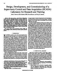
Figure 2.5 – Energy loss distribution in silicon for a sensor thickness of 200 μm.

43

42

MAZZIOTTA M. N., Electron-hole pair creation energy and Fano factor temperature dependence in silicon, in Nuclear Instruments and Methods Section A, Vol. 584, 2008, pp. 436-439.


41


The Landau distribution is asymmetric and it is characterized by a narrow peak and a long tail towards greater values. It can be mathematically described by the equation (2.4.); an equivalent form, more convenient for the computation, is given by equation (2.5.). p (x )

=

p (x )

=

1 c +i∞ s ⋅log s + xs ds ∫ e 2π i c −i∞ 1∞

π

− t ⋅log t − xt sin(π t ) dt ∫e

(2.4.)

(2.5.)

0

The Figure 2.5 shows the probability of energy loss in a silicon sensor with a thickness of 200 μm, as the one used in the SPD. The mean energy loss is that of a MIP (~60 keV), as described above. The information of the charge released inside the sensor by a MIP is important for the optimization of the detector readout chain.

2.2. Detector modules The Silicon Pixel Detector has a barrel structure that surrounds the beam pipe; it is made of 10 sectors that can be identified in Figure 2.6. According to the ALICE naming convention, the SPD barrel is divided, at z = 0, into two sides, called A and C. Each sector is a carbon fiber support structure that hosts 12 modules called half-staves (six per side), four of them on the inner layer in a staggered configuration, and eight on the outer layer in a windmill configuration. The inner layer is placed at an average distance of 3.9 cm from the beam axis (the minimum distance from the beam pipe is only ~0.5 cm); the outer layer is placed at 7.6 cm from the beam axis. In order to cover the full azimuthal angle, the detector modules need to have a small overlapping area.

43

OSMIC F., The ALICE Silicon Pixel Detector System, CERN-THESIS-2006-030, Geneva, CERN, May 2005, p. 21.


42


half-stave

Figure 2.6 - Silicon Pixel Detector seen from side A. On the left the real detector is shown; the inner layer, the extenders for power, the cooling lines and optical fibers for clock and readout are visible. On the right a 44 schematic view with the 10 sectors is shown.

The dimensions of the SPD are described in Table 2.1.

avg R (cm)

Z (cm)

Area (m2)

# of channels

Inner layer

3.9

14.1

0.07

3 276 800

Outer layer

7.6

14.1

0.14

6 553 600

Table 2.1 - Dimensions of the SPD.

The basic module of the SPD is the half-stave: it consists of two ladders, one Multi-Chip Module (MCM), and one multi-layer pixel bus. Each ladder is composed of one silicon sensor, bump bonded to five front-end chips. The individual elements of one half-stave are shown in Figure 2.7. Power extender

Pixel bus

Ladder

Ladder

Figure 2.7 - The elements of one half-stave.

44

MCM 45

From the SPD DATABASE website, http://pcal04.ba.infn.it/database/.


43


The silicon sensor (p-in-n type) has an active area of 70.7 mm x 12.8 mm. It is a matrix of cells with dimensions of 50 μm (rφ) x 425 μm (z), organized in 256 rows (rφ) and 160 (= 32 x 5) columns (z). The connection between each pixel of the sensor and the corresponding readout cell in the front-end chip is done using fine pitch flip-chip bonding. In order to reduce as much as possible the multiple scattering in the detector, the material budget has been kept to a minimum: the ALICE experiment requires that the material budget is ~1% X0 per layer, therefore the sensor has a thickness of 200 μm, and the front-end chip is thinned down to 150 μm after bump deposition. The two ladders are then glued to a multi-layer Al-Kapton bus (called pixel bus), 240 μm thick. Aluminum was chosen as conductor instead of copper to keep the material budget within the above described limitations. The connections between the chip pads and the pads on the bus are established using ultrasonic wire bonding. An aluminum bonding wire of 25 μm diameter has been adopted.

Figure 2.8 - Wire bonding connections between the ladders, the MCM and the pixel bus.

45

KLUGE A., et al., The ALICE Silicon Pixel Detector: electronics system integration, in IEEE Nuclear Science Symposium Conference Record, Vol. 2, 2005, pp. 761-764.


44


Figure 2.9 - Schematic of the wire bonds between the ladders, the MCM and the pixel 46 bus.

Figure 2.8 and Figure 2.9 show a picture and the schematic of the wire bonding connections between the bus and the front-end chip, respectively. Two layers of the pixel bus are used for the voltage supply and ground connections; three layers are used for the data and control signals. The different layers of the bus have different sizes to allow access to each layer for the wire bonds.

Two half-staves are then mounted on the sector carbon fiber support along the z direction to form a stave and there are six staves on each sector. As mentioned above, the entire SPD is made of 10 sectors, resulting in a total of 120 half-staves, 1200 front-end chips and ~9.8 x 106 pixels.

The detector and its front-end electronics dissipate a considerable amount of power of ~1.35 kW. An evaporative cooling system 47 based on Freon (C4F10) allows operating the detector at ambient temperature.

46

KLUGE A., et al., The ALICE Silicon Pixel Detector (SPD), in Proceedings of the th 8 International Conference on Advanced Technology and Particle Physics, Como, Italy, Sep 2003. 47 ALICE COLLABORATION, The ALICE experiment at the CERN LHC, in Journal of Instrumentation, Vol. 3, Geneva, CERN, Aug 2008.


45


Each sector is equipped with six cooling capillaries, embedded in the carbon fiber support structure and in thermal contact with each stave by means of thermal grease. Due to the low mass of the system, in case of a cooling failure the temperature of the system would increase by 1 °C/s. Therefore the temperature is a critical parameter for the SPD that has to be monitored continuously.

Two independent chains of five temperature sensors (PT1000) each are mounted as Surface Mounting Device components on the pixel bus of each half-stave, and they are used to monitor the temperature in a redundant configuration to increase the safety level. One chain is hard-wired and read with a dedicated PLC system, the other is read through the Multi Chip Module and the SPD off-detector electronics. Both chains are connected to an interlock system that automatically switches off the half-stave if its temperature exceeds a certain threshold. It consists of several interlock levels: •

hardware interlock: the readout chain based on the PLC is hardwired to the remote interlock system. The PLC scans all the 120 halfstaves in less than 1 s. In case the temperature of one half-stave exceeds the predefined threshold (typically ~41 °C), the low voltage power supply of the corresponding half-sector is switched off;

•

software interlock: slower than the hardware interlock, it is based on the temperature readout in the off-detector electronics, in this case only the single half-stave that has a temperature exceeding the set threshold is switched off. For the software interlock the threshold is lower than the one used for the hardware interlock, typically ~39 °C.

2.3. Front-end chip The front-end chip of the SPD is called ALICE1LHCb, and it is a mixed


46


signal ASIC 48 developed in an IBM 0.25 μm CMOS process 49; the chip size is 13.5 mm x 15.8 mm, including internal DACs, chip controls and pads for wire bonding.

The pixel detector is placed very close to the interaction point in the experiment; the total radioactive dose expected during the lifetime of the experiment (10 years) is ~ 270 krad for the inner layer, and ~70 krad for the outer layer, with a 1 MeV neutron equivalent fluency of 3.5 x 1012 cm-2 for the inner layer and 1.3 x 1012 cm-2 for the outer layer 50. In addition to using a 0.25 μm CMOS process the chip was radiation hardened by design layout, such as by using gate all around designs and guard rings.

Figure 2.10 - Block diagram of the circuitry in one cell of the front-end chip.

51

48

Application-Specific Integrated Circuit, it is an integrated circuit customized for a particular use. The modern ASICs can have from 5000 to 100 million gates, and normally they include 32-bit processors and memories (ROM, RAM, EEPROM, etc.). They are programmed with hardware description language, and the most common standards are VHDL or Verilog. 49 WYLLIE K., et al., Front-end pixel chips for tracking in ALICE and particle th identification in LHCb, in Proceedings of the 5 Workshop on Electronics for LHC Experiments, Colorado, USA, Sep 1999. 50 ALICE COLLABORATION, The ALICE experiment at the CERN LHC, in Journal of Instrumentation, Vol. 3, Geneva, CERN, Aug 2008. 51 From The ALICE Silicon Pixel Detector website, http://aliceinfo.cern.ch/Public/en/Chapter2/Chap2_SPD.html.


47


The front-end chip works at a frequency of 10 MHz, thus the clock cycle is 100 ns. This is the bunch crossing frequency set by the LHC for the ALICE experiment during heavy-ion operation 52, while the bunch crossing spacing during the operation with protons is 25 ns. The front-end chip has a matrix structure of 256 (rows) x 32 (columns) cells, with size 50 μm (in the rφ plane) x 425 μm (along z); each cell contains the circuitry shown in Figure 2.10.

Each cell has an analogue and a digital part. The analogue part 53 contains a preamplifier, two shaper stages, and a discriminator that digitalizes the signal. The amplifier and the shapers are of a differential type, to improve the rejection of the common mode noise (i.e. substrate and supply noise). The shapers tune the signal peaking time to 25 ns. The readout of the detector is binary: in each pixel a threshold is applied to the pre-amplified and shaped signal and the digital output level changes when the signal is above the set threshold. After the discriminator there is a synchronizer block that synchronizes the signal with respect to the 10 MHz internal clock of the SPD front-end chip.

The digital part has two 8-bits delay lines; each of them stores the hit information for the duration of the trigger latency, and can delay the signals of up to 512 clock cycles. On reception of a L1 trigger, the signal is sent to one of the four positions of a Multi Event Buffer (MEB). After a Level 2 accept trigger is received, the readout sequence is initiated and the data is sent to the following flip-flops. The readout is done via a 32-bit data bus, so one row per clock cycle is read. The time needed to readout one half-stave (10 chips) is then 100 ns (clock cycle) x 256 (rows) x 10 (chips) = 256 μs

52

ALICE COLLABORATION, ALICE: Physics Performance Report Volume 1, in Journal of Physics G: Nuclear and Particle Physics, Oct 2004, p.1586. 53 DINAPOLI R., An analog front-end in standard 0.25 μm CMOS for silicon pixel detectors in ALICE and LHCb, in Nuclear Instruments and Methods Section A, Vol. 461, Elsevier, Apr 2001, pp. 492-495.


48


This is also the time needed for the readout of the entire SPD detector, because the 120 half-staves are read in parallel.

In order to simulate a particle crossing the pixel, a test pulse can be applied to the input of each cell via a capacitor. In each pixel, a capacitance (C test) is put in series with the input of the preamplifier, as shown in Figure 2.10; the pixel can be set in TEST mode with an internal flip-flop, in this case the capacitance is connected to the input through CMOS switches; otherwise, if the pixel is in data taking mode, the capacitance is shorted and disconnected. The value of the capacitance is 16 fF; this type of capacitor has by design a high tolerance, of the order of 15%. After measurements with a

55

Fe source in the laboratory, it has been found

that the conversion factor between voltage and charge is 1 mV ≅ 70 electrons. Two DC levels, called TEST_HI and TEST_LOW, are provided from outside the front-end chip by an integrated circuit (Analog Pilot, see paragraph 2.4.). Using a digital control signal, called TestPulse, the capacitance is connected alternatively to TEST_HI and TEST_LOW, simulating a charge injection of a voltage pulse of a know amplitude equal to TEST_HI – TEST_LOW. This process is schematically shown in Figure 2.11.

Figure 2.11 - Schematic representation of the chip internal pulser.

The input pulse is created in an inverted way with respect to the TestPulse input: if the TestPulse signal is high, then the capacitor is connected to the TEST_LOW value, while if the TestPulse is low the capacitor is connected to the TEST_HI value. The switches that determine whether the test pulse is applied to the pixel or not are PMOS transistors: if TEST_LOW is lower than 0.8 V, the resistance of the switch increases and the pulse signal saturates.


49


The test pulse signal is then propagated from column 5 to all pixels inside the chip matrix. The duration of the test pulse is 200 ns; since the discriminator is sensible to both transitions of the input signal (low-high and high-low), the test pulse has to be longer than 100 ns (one clock cycle) to avoid the detection of the trailing edge.

The front-end chip has many parameters that can be remotely adjusted. Inside the chip there are 42 8-bit DACs that can be individually tuned for the detector operation and optimization; they act, for example, on voltage and current references, delays and readout threshold. An example of the functioning of these DACs is given in section 2.3.1. On each half-stave the configuration parameters are controlled by the Digital Pilot, which is located on the MCM, with a JTAG standard interface. A detailed description is given in section 3.4.

2.3.1. Fast-OR circuitry The SPD has the capability to produce a Fast-OR signal that can contribute to the first level trigger of ALICE (Level 0); this is a unique feature among the other silicon vertex detectors of the LHC experiments. The Fast-OR signal is generated on a chip basis: each of the 1200 front-end chips can activate its Fast-OR output if at least one pixel inside that chip is hit by a particle. The 1200 Fast-OR bits are transmitted every 100 ns to the off-detector electronics (Routers) by the Multi Chip Module.

The SPD trigger signal is called Fast-OR because it is generated as a logical OR of all the pixel cells inside one front-end chip, and because it has a low latency: the Fast-OR is produced after the discriminator and it is sent immediately to the off-detector electronics, without further processing in the readout cell. The Fast-OR circuitry is visible in Figure 2.12.


50


Figure 2.12 - Schematic of the Fast-OR circuitry.


51


The Fast-OR circuitry of each front-end chip is controlled by four DACs; the DAC settings affect the efficiency, the uniformity and the noise immunity of the circuitry, as explained in the table below.

DAC name

Function

Fast_CGPOL

Transconductance fine tuning

Fast_COMPREF

Comparator reference at the end of the Fast-OR chain

Fast_CONVPOL

Current mirror voltage bias

Fast_FOPOL

Current pulse source

Table 2.2 - DACs of the Fast-OR circuitry.

Inside each pixel cell, the Fast-OR signal is produced via a P-MOS transistor. The current applied at the source is regulated by the Fast_FOPOL DAC, and the signal coming from the discriminator is applied at the gate. Due to the circuitry of the synchronizer, at this stage the signal is only ½ clock cycle long, i.e. 50 ns.

Figure 2.13 - Generation of the Fast-OR signal inside each pixel cell.

Then the current signals of all pixel cells are grouped by column. The circuitry at the end of column is shown in Figure 2.14.


52


Figure 2.14 - Collection of the Fast-OR signals at each end of column.

The intensity of the current injected in the circuit is regulated by the Fast_CONVPOL DAC; a decrease in the DAC value corresponds to an increase of the current in the Fast-OR circuit. At the end of each column, the signals coming from the corresponding 256 pixels are summed in OR, and they are compared with a threshold that depends on Fast_COMPREF. A high Fast_COMPREF value corresponds to a low threshold. The signals coming from the 32 columns are then summed together with a similar circuitry placed at the Fast-OR pad at the chip edge.

Figure 2.15 - Fast-OR pad of the chip, collecting the signals coming from the 32 columns.


53


The signal is again discriminated and compared with a threshold that depends on Fast_COMPREF.

When one pixel is hit inside a chip, the related Fast-OR signal arrives to the Fast-OR pad one clock cycle (100 ns) later. The amplitude of the final output pulse depends on Fast-CONVPOL, while its width depends on Fast-COMPREF, as visible in Figure 2.16.

Figure 2.16 - Fast-OR signal generated at the chip output. The effect of Fast_COMPREF and Fast-CONVPOL are indicated.

The analysis and regulation of the Fast-OR DACs provides an important tool to optimize the trigger signal, as explained in chapter 4.

2.3.2. Delay settings When a particle hits the detector, the signal is synchronized to the 10 MHz internal clock; inside the delay lines the pulse is delayed by an integer number of clock cycles and the duration of it can be programmed with the Delay_control register, settable by a dedicated DAC of the front-end chip.


54


If D is the numeric value set in the Delay_control register, then the delay corresponds to Delay = (2*D + 2) * 100 ns [ns]

(2.6.)

Since the DAC has 8 bits, the maximum delay that can be applied to the pulse is Max delay = (2*255 + 2) * 100 ns = 51.2 μs

(2.7.)

The signal is stored in the delay line waiting for the L1 trigger coming from the ALICE Central Trigger Processor. The L1 trigger signal is sent in parallel to the MCMs; there the trigger is translated into a strobe signal that is applied to all front-end chips. The duration of the strobe window is programmable and can be changed with the Strobe_length register of the MCM. If S is the numeric value set in the Strobe_length register, then the strobe duration is given by the following equation:

Strobe = (S + 1) * 100 ns [ns]

(2.8.)

As an example, a setting of 0 corresponds to a strobe length of 100 ns, a setting of 2 to a strobe length of 300 ns. These are the two settings that are usually used during the data acquisition.

The strobe window can also be delayed of 100 ns inside the chip; this is done changing the Misc_setting register of the front-end chip. This register can only assume values 128 (in binary 10000000) or 192 (in binary 11000000). The value of the second most significant bit is used to activate the delay or not.

Changing the delay control, misc control and strobe length registers, the strobe readout window can be timed with the presence at the output of the delay lines of the pulse generated by a particle inside the detector.


55


If the synchronization is correct and all the latencies introduced by the trigger electronics and the trigger transmission are considered, then the hit information can be seen in the readout. In case of a 100 ns strobe length, the delay that has to be set corresponds to

Delay = Latency + Misc * 100 [ns]

(2.9.)

Inverting the equation, it is possible to determine the latency values that correspond to the different delay settings

Latency = Delay - Misc*100 = (2*N + 2) * 100 - Misc*100 [ns]

(2.10.)

Table 2.3 gives an example of delay settings and the corresponding latencies for a strobe length of 100 ns.

Latency [ns]

Delay_control Misc_control

10300 ÷ 10400

51

192 [1]

10400 ÷ 10500

51

128 [0]

10500 ÷ 10600

52

192 [1]

10600 ÷ 10700

52

128 [0]

10700 ÷ 10800

53

192 [1]

10800 ÷ 10900

53

128 [0]

10900 ÷ 11000

54

192 [1]

11000 ÷ 11100

54

128 [0]

Table 2.3 - Delay settings and the corresponding latency of the pulse inside the chip.

Considering the real latencies of the experiment, the settings used are 53 for Delay_control and 192 for Misc_control.

2.4. Multi Chip Module The Multi Chip Module (MCM) is a five layer Kapton-based module that


56


controls the front-end chips on one half-stave. It provides timing, trigger and control signals to the 10 chips of the half-staves and contains four ASICs: • Analog Pilot (ANAPIL) 54: it monitors currents and voltages and it gives reference voltages to the pixel chips. It also monitors the temperature of the half-stave; • Digital Pilot (PILOT2003) 55: it initiates the readout of the front-end chips and transmits the data to the off-detector electronics. It also provides the clock and the configuration commands to the half-stave; • Gigabit Optical Link (GOL) 56: it serializes/de-serializes the data and it controls the laser used for the communication trough the optical fibers, sending the data out at 800 Mbit/s; • RX40 57: the optical receiver, which converts the optical signals into electric ones. All four ASICs are built with the same 0.25 μm C-MOS technology as the front-end chip.

Figure 2.17 - Multi Chip Module. From left to right: ANAPIL, PILOT2003, GOL, RX40. The black box on the right is the optical package containing two diodes and one laser for 58 the data handshake with the back-end electronics.

Each MCM is connected to the back-end electronics via three single mode optical fibers designed for 1310 nm wavelength: two of them are used to receive the serial control for the commands and the LHC clock at 40.08 MHz

54

POWELL A. S., Analogue Pilot testing, in LHCb RICH L0 Production Readiness Review, Geneva, CERN, 2004. 55 KLUGE A., ALICE Silicon Pixel On Detector Pilot System OPS2003 - The missing manual, ALICE Internal Note, ALICE-INT-2004-030, Geneva, CERN, 2004. 56 MOREIRA P., et al., A 1.25 Gbit/s serializer for LHC data and trigger optical links, in Proceedings of Fifth Workshop on Electronics for LHC Experiments, CERN/LHCC/99-33, Oct 1999, pp.194-198. 57 FACCIO F., et al., RX40 An 80 Mbit/s optical receiver ASIC for the CMS digital optical link, Geneva, CERN, Oct 2001. 58 KLUGE A., et al., The ALICE Silicon Pixel Detector: electronics system integration, in IEEE Nuclear Science Symposium Conference Record, Vol. 2, 2005, pp. 761-764.


57


(Serial and Clock), the third one is used to transmit the data flow (Data or Glink). In order to reduce the material budget and due to the space constraints, the Digital Pilot, the Analog Pilot and the GOL chips are mounted as unpackaged dies.

The transmission of digital data from the SPD to the back-end electronics and the data acquisition system is done with unidirectional links: the transmitters are located on the detector and need to be radiation tolerant to withstand the radiation doses expected during the lifetime of the experiment, while the receivers are located in the control room in a non-radiation environment. ALICE chose to make its custom made transmitter compatible with existing communication standards; in particular the SPD uses the G-Link protocol59, synchronous and thus appropriate for data links that should be synchronized with the LHC clock.

2.5. Off-detector electronics The SPD off-detector electronics is located in a control room called CR4 (floor -4 with respect to ground level), at about 100 m from the detector. There, two VME crates dedicated to the SPD host 20 9U-VME boards called Routers 60 that control, configure and monitor the data taking of the SPD. Each Router controls 6 half-staves from one half-sector; the interface with the half-staves is constituted by three plug-in daughter cards called Link Receiver (LinkRx) cards, mounted on the Router boards.

59

YEN C. S., et al., G-Link : a chipset for gigabit-rate data communication, in Hewlett-Packard Journal, Oct 1992, pp.736-753. 60 KRIVDA M., The ALICE silicon pixel detector readout electronics, in Proceedings of LECC 2006, Valencia, Sep 2006.


58


LinkRx

Figure 2.18 - SPD Router board. The three LinkRx are visible on the left side.

61

The LinkRx contains one commercial FPGA that sends the trigger and the configuration data and receives the data stream coming from the detector. The data stream is deserialized, stored in a FIFO and zero-suppressed; then it is reformatted and written in a Dual Port Memory (DPM).

Figure 2.19 - Block diagram of the MCM and Router connections.

61

From the SPD router page website, http://aliceinfo.cern.ch/SPD/Detector/Electronics/Router.html.


59


The schematic of the communication between the Router and the MCM is shown in Figure 2.19. The Router transmits the data stream to the ALICE Data Acquisition (DAQ) system through the ALICE standard Detector Data Link (DDL) 62. The Routers communicate also with the Detector Control system (DCS), which is responsible of the detector configuration, via the VME bus.

2.6. SPD control system For the correct operation of the on-detector and off-detector electronics, ~2000 parameters and ~50000 DACs have to be set and monitored online. The detector is controlled and operated by the Detector Control System (DCS) 63, a distributed control system whose aim is to control and operate the ALICE experiment during all modes of operation. It provides interfaces for the users, and communicates with external systems such as databases and the ALICE Detector Control System 64.

The SPD DCS comprises three PVSS control nodes and two Front End Device (FED) servers. The PVSS 65 (in German it stands for Prozess-Visualisierungs und SteuereungsSystem, or Process Visualization and Control System) control nodes constitute a supervisory layer designed in the SCADA (Supervisory Control And Data Acquisition) language. They control the overall status of the detector, provide configuration data, and take the appropriate corrective action in order to maintain the stability of the system and to ensure the data quality.

62

DIVIA’ R., et al., Data format over the ALICE DDL, ALICE Internal Note, ALICEINT-2002-010, Geneva, CERN, 2004. 63 CALÌ I. A., et al., The ALICE Silicon Pixel Detector control system and on-line calibration tools, in Journal of Instrumentation, Vol. 2, Apr 2007. 64 CHOCULA P., et al., The ALICE Detector Control System, in IEEE Transactions on Nuclear Science, Vol. 52, Apr 2010, pp. 472-478. 65 From the ETM website, http://www.etm.at/. More information is available here.


60


The data is exchanged real-time with external services and systems through a standard interface based on the CERN Data Interchange Protocol (DIP) 66.

The supervision layer of the SPD connects the PVSS layer with the detector front-end electronics, and it is composed by three different projects, shown in Figure 2.20: •

spd_a: it controls the power supplies (manufactured by CAEN S.p.A.) and the Finite State Machine (FSM) for the half-staves of side A;

•

spd_c: it controls the power supplies and the FSM for the half-staves of side C;

•

spd_dcs: it is a top level project that controls the SPD cooling plant, the VME crates, the CAEN supply mainframe and the communication with the FED servers.

Figure 2.20 - Diagram of the SPD Detector Control System.

66

SALTER W., LHC Data Interchange Protocol (DIP) Definition, EDMS document 457113, Geneva, CERN, 2004.


61


2.6.1. SPD Front End Device The Front End Device (FED) server of the SPD (called spdFed) is a C++ based applications that are designed to be the driver layer of the SPD detector. It interfaces with the on-detector and off-detector electronics, sending commands for the configuration, performing calibration procedures and publishing the status information.

The FED servers consist of three software layers: the top one contains a server that allows the communication with the PVSS system, the intermediate layer contains the FED state machine and all the functions required for the operation of the detector, the bottom layer contains the driver for the VME access of the off-detector electronics. There are two clones of the FED servers, one per side, and each of them accesses the 32-bit VME bus of one Router crate.

The communication between the two FED servers and the PVSS interface is carried out by the Distributed Information Management (DIM) system 67, developed at CERN. DIM is a protocol for distributed environments, which provides an interprocess communication layer. It is based on the server/client paradigm, and on the concept of services: servers provide services to the clients. The relations between servers and clients are shown in Figure 2.21; the name servers keep track of all the servers and services available in the system. The command structure of the spdFed servers is flexible and it can manage a variable number of arguments and display the status of the execution of all commands.

67

From the DIM website, http://dim.web.cern.ch/dim/.


62


Figure 2.21 - Interactions between the DIM components.

The command channel of each spdFed server is composed of three DIM commands and five DIM services. •

DIM commands: −

COMMAND_NAME: a string that identifies the command to be executed;

−

CHANNEL_NUMBER: the number of the half-stave where the command has to be executed; if a command is for one entire Router, it can be the number of any of the half-staves of this Router;

−

DATA_IN: an array of variable length that contains the input data of the command; the format of the data depends on the type of command that is sent;

•

DIM services: −

RET_DATA: an array of variable length with the output data of the last command;

−

ERROR_CODE: an integer value that displays the status of the execution of the last command;

−

ERRORS_REPORT: a string with detailed information of the execution status of the last command;


63


−

CMD_NAME: it returns the command name;

−

CH_NUMBER: it returns the channel number.

The communication layer also hosts a pooling object that performs cycling operations such as temperature reading and Routers memory reading. The complex operations such as calibrations that are done by the SPD FED are divided into steps, and at the end of each step the control is given to the pooling object that decides the request to execute.

The two servers are stand-alone applications that can run on Windows or Linux machines, and they are Visual Studio 2003 solutions based on the following six projects: •

ALICE_SPD_DIMServer: top level project, it contains the DIM interface to communicate with PVSS and parses all the commands to/from the FED;

•

HSConfig: dedicated to the configuration of the half-staves, it contains high level classes to manage the half-staves and Routers configuration and the calibration scans;

•

AddressGenerator: it contains classes to access the memory addresses of the Routers and Link Receivers;

•

BitsManager: it is dedicated to bitwise operations;

•

spdDbConfLib: manages the SPD database, it contains classes to connect to the database and to manage the versioning system;

•

VMEAcc: low level project that controls the access to the VME bus, it contains classes for the reading and writing of the VME registers.

Figure 2.22 - Dependencies of the SPD FED server projects.


64


Figure 2.22 shows the projects dependencies. The development of the Level 0 pixel trigger system required adding new functionalities and new classes inside the two SPD FED servers, maintaining the existing projects structure.


65

3. The ALICE Pixel Trigger system __________________________________________________________________________

3. The ALICE Pixel Trigger System The Pixel Trigger 68 (PIT) processes the 1200 Fast-OR signals (one per frontend chip) generated by the SPD, and it delivers an input to the ALICE Central Trigger Processor (CTP). The latency of the Pixel Trigger signal is such that it contributes to the Level 0 trigger decision. The integration of the Pixel Trigger inside the ALICE experiment is shown in Figure 3.1.

Figure 3.1 - The Pixel Trigger integrated with the detector electronics and the DAQ system.

68

ALICE COLLABORATION, The ALICE experiment at the CERN LHC, in Journal of Instrumentation, Vol. 3, Aug 2008.


66


From the trigger point of view, the SPD can be considered as a low latency and low granularity detector, with an equivalent pad size of ~ 13 x 14 mm2, corresponding to the size of one chip. For the detectors that contribute to the L0 trigger, the ALICE experiment requires that the latency between the head-on beam interaction, i.e. the bunch crossing, and the trigger input to the CTP is less than 800 ns 69. For this reason, the trigger system must be placed as close as possible to the detector and the CTP. The CTP racks are located inside the cavern, under the muon arm, about 50 m away from the detector, and the Pixel Trigger is located in a rack next to the CTP.

Figure 3.2 - Pixel Trigger system inside the ALICE cavern; the Pixel Trigger crate (below) and the optical splitters (above) are visible.

69

ALICE COLLABORATION, ALICE Technical Design Report of the trigger, data acquisition, high-level trigger and control system, Geneva, CERN, Jan 2004, pp.1770.


67


The Fast-OR bits are embedded in the data stream coming out from the detector on the 120 G-link optical fibers (one per half-stave, see paragraphs 2.3. and 2.4.). The G-links are therefore connected to 120 passive optical splitters, placed in the same rack as the Pixel Trigger, shown in Figure 3.2; one output of the splitter is connected to the Pixel Trigger, while the other output is connected to the Routers (back-end electronics) located in the control room in CR4, ~100 m away. This allows the readout path of the SPD to be fully independent from the Pixel Trigger.

In addition to the latency requirement, the Pixel Trigger has to •

extract the 1200 Fast-OR bits from the data stream of the SPD;

•

collect the 1200 bits in a processing FPGA;

•

process the bits with algorithms that can be selected depending on the type of run and configured from remote;

•

be controllable and configurable by the ALICE Detector Control System (DCS).

These specifications led to a modular design that includes a central processing board and some receiver boards. The Pixel Trigger is divided into two sub-systems 70: •

OPTIN boards: the receiver boards that deserialize the data stream coming from the SPD and extract the Fast-OR bits. The PIT contains 10 OPTIN boards mounted on the central board;

•

BRAIN board: the central processing board that applies processing algorithms on the bits and generates the outputs for the CTP.

3.1. OPTIN board The OPTIN boards are the receiver

boards

that

implement the

deserialization and extraction of the Fast-OR bits from the SPD data stream

70

AGLIERI RINELLA G., et al., The Level 0 Pixel Trigger system for the ALICE experiment, in Journal of Instrumentation, Vol. 2, Jan 2007.


68


(G-Link protocol). Each board has a customized optical receiver module with 12 channels that is able to receive the data coming from 12 half-staves (two half-sectors). The Pixel Trigger is

equipped with 10 OPTIN boards

and the

correspondence with the SPD sectors is shown in Table 3.1.

OPTIN

Half sector

OPTIN

0A

0

2A 4A 6A

3C 4C 5C 6C

8

7A 8A

4

2C

7

5A

3

1C

6

3A

2

0C

5

1A

1

Half sector

7C 8C

9

9A

9C

Table 3.1 - Correspondence between the OPTIN boards and the SPD half-sectors.

The optical receiver module converts and amplifies the optical signals, and it is connected to 12 single channel deserializer ASICs 71 that send the signals to an FPGA 72 (Field Programmable Gate Array). The FPGA receives the deserialized signal, decodes the G-Link protocol and extracts the Fast-OR bits, transmitting the output on a parallel bus to the main board. The block diagram of the OPTIN board is shown in Figure 3.3. The use of a parallel bus is mandatory because of the stringent requirements

on

the

latency

of

the

trigger

system;

a

serialized

communication would exceed the allowed latency. The signals are transmitted from the OPTIN board to the BRAIN board every 100 ns with a double data rate transfer (time division multiplexing).

71

From the All Datasheets website, http://www.alldatasheet.com/datasheet-pdf/pdf/113224/HP/HDMP-1034.html. The datasheet of Agilent HDMP-1034 is available here. 72 From the Xilinx website, http://www.xilinx.com/support/documentation/data_sheets/ds112.pdf. The datasheet of Xilinx Virtex 4 LX60 is available here.


69


Figure 3.3 - Block diagram of the OPTIN board.

Figure 3.4 - OPTIN board. The optical receiver, six deserializers and the FPGA are 73 shown; the other six deserializers are mounted on the other side of the board.

The architecture of the OPTIN boards is determined by the choice of the optical receiver module and the use of 12 ASICs; it is realized on a 12 layer printed circuit board with dimensions of 160 x 84 mm2, visible in Figure 3.4. While the SPD detector runs with a 10 MHz internal clock, the Pixel Trigger works at the LHC clock frequency of 40 MHz.

73

AGLIERI RINELLA G., Development and implementation of the Level 0 Pixel Trigger system for the ALICE Silicon Pixel Detector, in IEEE Nuclear Science Symposium Conference Record, 2007, pp. 2141-2144.


70


3.2. BRAIN board The BRAIN board receives the Fast-OR bits from the OPTIN boards and processes them, sending the output to the CTP. It is a 9U (400 x 360 mm2) size board, as shown in Figure 3.5.

Figure 3.5 - BRAIN board. Two OPTIN boards are visible on one side of the board. The Processing and the Control FPGAs are shown and the output connectors are also 74 visible.

The OPTIN boards are mounted on the two sides of the BRAIN board as mezzanine cards. In this way the assembly is compact and the routing of the signals is simplified, avoiding the wired interconnections. The BRAIN board contains a large FPGA 75, called Processing FPGA, with 1513 pins. The large number of pins and the space it occupies are due to the high number of parallel lines that transfer the Fast-OR bits from the OPTIN boards: each OPTIN has 64 lines dedicated to the Fast-OR signals that reach dedicated inputs of the Processing FPGA.

74

AGLIERI RINELLA G., Development and implementation of the Level 0 Pixel Trigger system for the ALICE Silicon Pixel Detector, in IEEE Nuclear Science Symposium Conference Record, 2007, pp. 2141-2144. 75 From the Xilinx website, http://www.xilinx.com/support/documentation/data_sheets/ds112.pdf. The datasheet of Xilinx Virtex 4 LX100 is available here.


71


Ten Low-Voltage Differential Signaling (LVDS) output lines transmit the processing results to the CTP.

The Processing FPGA processes the Fast-OR bits with different algorithms at the same time, based on multiplicity, which are implemented using Boolean functions. The maximum number of algorithms that can be implemented is limited by their complexity and the available logic resources inside the FPGA. In any case, the Pixel Trigger has 10 output lines, so the maximum number of the implemented algorithms is 10. All the algorithms implemented are completed in one clock cycle, i.e. 25 ns only. A detail of the algorithms is given in Table 3.2.

PIT output

Trigger name

0

0SMB

Minimum bias

Ntot >= total && Nin >= inner && Nout >= outer

1

0SH1

High multiplicity

Nin >= inner && Nout >= outer

2

0SH2

High multiplicity


3

0SH3

High multiplicity


4

0SH4

High multiplicity


5

0SPF

Past-future protection

Ntot >= total && Nin >= inner && Nout >= outer

6

0SX1

Spare background

Nin >= Nout + offset inner layer

7

0SX2

Spare background

Nout >= Nin + offset outer layer

8

0SBK

Background

Ntot >= background both layers

9

0SCO

Cosmic

Programmable

Description

Trigger logic

Table 3.2 - Algorithms implemented in the Processing FPGA.

The minimum bias trigger can be used to select proton-proton collisions with high efficiency, providing a rejection of the background due to the interaction of incoming protons with the residual gas in the beam pipe.


72


The multiplicity algorithms can also be used for background rejection or to select high multiplicity events 76.

The output 9 of the Pixel Trigger corresponds to the algorithm used to detect cosmic rays. For this particular output, the choice of the trigger logic that has to be used is selectable by the operator. Table 3.3 lists the possible choices.

Selector

Trigger logic

0

top outer && bottom outer

1

inner layer && outer layer

2

>= 2 FO in the inner layer && >= 2 FO in the outer layer

3

top outer && top inner && bottom outer && bottom inner

4

top outer && bottom outer && inner layer

5

global OR

Table 3.3 - Possible selection for the cosmic algorithm.

At the output of the Processing FPGA, the signal is synchronized with the 10 MHz clock of the detector and integrated over 100 ns. During the 100 ns there can be 4 bunch crossings with proton-proton interactions, and 1 bunch crossing with heavy ions. This may lead to pile-up between consecutive events during normal LHC operation. In the ALICE trigger system this ambiguity can be resolved putting the Pixel Trigger output in coincidence with the output signal of the V0 detector, which has a 25 ns time resolution. The combination of the two signals is also useful because of the complementarity of the two detectors in geometrical acceptance: the SPD covers the central region, while V0 covers the forward region on the two sides of the interaction point.

On the BRAIN board is also mounted another FPGA, called Control FPGA, that provides control and communication functionalities. It acts as a bus

76

ELIA D., et al., The pixel Fast-OR signal for the ALICE trigger in proton-proton collisions, in International Journal of Modern Physics section E, World Scientific Publishing Company, Vol. 16, 2007, pp. 2503-2508.


73


master, controlling the 32-bit bus used for the communication between all the FPGAs of the OPTIN and BRAIN boards. The communication between the Pixel Trigger electronics and the remote controlling machine is done with a Detector Data Link (DDL). The DDL Source Interface Unit (SIU) is also visible in Figure 3.5 and it is connected to the Control FPGA, which is the bridge between the DDL and the bus on the Pixel Trigger board.

3.3. Pixel Trigger control system Similarly to the SPD, also the Pixel Trigger is controlled by the DCS (Detector Control System), with an interface for the users realized in PVSS, one driver and databases.

Figure 3.6 - Interconnections of the PIT Control System with the ALICE subsystems.

The control system of the Pixel Trigger is located in Control Room 3 (CR3, at floor -3 with respect to ground level) and it is composed by 2 computers: a


74


Windows PC with the supervision layer, and a Linux PC with the driver layer, called pitFed server. As shown in Figure 3.6, it interfaces with the other ALICE subsystems such as •

the Detector Control System of the SPD, with whom it exchanges data during calibration scans;

•

the Central Trigger Processor, from which it receives configuration commands;

•

the Experimental Control System (ECS), to which it sends status information.

The supervision layer is based on PVSS, the SCADA (Supervisory Control And Data Acquisition) adopted in ALICE; it controls the trigger status and it takes corrective actions in order to maintain the stability of the system and to ensure the required trigger quality. Similarly to the spdFed, the pitFed server is developed in C++ and it is structured as the driver layer of the PIT system: it checks the trigger quality, it provides hardware debugging tools and it publishes status services for alarm information. It was developed using CERN standard libraries: •

DIM: it is used to publish information and receive commands from other computers through the network;

•

OCCI: it is used to access the database that store the information of the chips included in the trigger logic and the parameters of the processing algorithms;

•

Log4cpp: it is used for the logging of all the commands received and the operations done by the PIT;

•

Fec2Rorc: it is used by the lower level of the software to communicate with the hardware.

The pitFed driver communicates with the Pixel Trigger hardware through the DDL link, and it communicates with PVSS through the DIM interface, publishing a list of services that displays information that are relevant to monitor the stability of the trigger system.


75


The command channel of the pitFed is designed to be flexible, so that it can receive commands from different ALICE subsystems with a variable number of arguments; it is composed of one DIM command and three DIM services: •

DIM command: −

COMMAND: a string with the name of the command to be executed;

•

DIM services: −

CMD_RETURN: an integer with the return value of the command;

−

CMD_STATUS: a string with the status of the command execution;

−

CMD_ID: an integer corresponding to one unique ID of the command that is currently being executed.

As described in the following chapters, the development of the Pixel Trigger System required an integration of new functionalities both in the spdFed and pitFed.


76

4. Development of a prompt L0 pixel trigger system __________________________________________________________________________

4. Development of a prompt L0 Pixel Trigger System The Pixel Trigger System is a versatile system that allows to provide a prompt L0 trigger to the ALICE experiment.

In order to define a stable

trigger signal provided by the pixel chips, a complete calibration procedure had to be defined and worked out as described in this chapter. As explained in paragraph 2.3.1., each front-end chip contains four DACs to control the efficiency, uniformity and noise immunity of the Fast-OR circuitry. The study and the optimization of the 120 half-staves of the whole SPD are is required in order to •

maximize the sensitivity of the detector to single hits;

•

minimize the readout noise of the Fast-OR signal.

This has to be done individually for each of the 1200 front-end chips.

The Fast-OR output of the front-end chips was initially foreseen for diagnostic purposes during the testing procedures and for self triggering. Thanks to the development of the Pixel Trigger System and the tuning and optimization of the trigger signal, described in this thesis, the Fast-OR output of the chips plays now an important role inside the ALICE experiment: the majority of cosmic rays and particle collision runs were recorded using the SPD trigger.

4.1. Manual tuning procedure The tuning procedure for the Fast-OR signal uses the possibility to apply a test pulse in every pixel inside the chip matrix (see paragraph 2.3.). The amplitude of the test pulse is set to 100 mV, in order to simulate the charge generated by a Minimum Ionizing Particle crossing the sensor. The test


77


pulse circuitry can be activated in each single pixel independently of the others, and the Fast-OR signal can be studied at the level of a single pixel. The tuning of the Fast-OR signal is based on a comparison between the number of test pulses that are sent to a pixel, and the number of Fast-OR pulses that are detected at the input of the Pixel Trigger for the corresponding chip. Three different conditions may happen: •

# test pulses > # Fast-OR signals -> inefficient pixel;

•

# test pulses = # Fast-OR signals -> efficient pixel;

•

# test pulses < # Fast-OR signals -> noisy pixel.

In this chapter the inefficient, efficient or noisy behavior of one pixel or chip has to be intended only as trigger related; the efficiency of the readout chain is studied in chapter 5.

The tests on the Fast-OR circuitry and a possible calibration method of its DACs were at first carried out in the laboratory, and then the knowledge acquired was applied on the detector installed in ALICE. A fully automatic procedure was developed and embedded in the SPD software driver.

4.1.1. Tests and measurements in the laboratory An initial study for the tuning of the Fast-OR parameters has been performed in the laboratory, in order to study the behavior of the circuitry responsible of the triggering and to model the impact of the DAC settings on the Fast-OR signal. The SPD laboratory is located inside the Divisional Silicon Facility (DSF) at CERN; the DSF is a common project launched to support the research activities for the LHC project, with clean rooms available for all experiments. The clean rooms have a controlled level of contamination, achieved with the use of filters and air pumps; the room dedicated to the testing of the SPD


78


was designed according to the international standard US FED STD 209E 77 to be class 100˙000: the maximum number of particles per cubic feet with size greater than 0.5 μm is 100 ˙000.

In 2001 this standard has been

replaced by the international standard ISO 14644-1 78, and the corresponding class for the SPD clean room is ISO 8. Inside the DSF the setup installed in the experiment is reproduced on a smaller scale: it includes some half-staves, the complete readout chain and the trigger control system, a cooling system and the power supplies.

Figure 4.1 - Setup in the DSF.

The auxiliary systems are the same model as used in the experiment:

77

US Federal Standard 209E, Airborne Particulate Cleanliness Classes in Cleanrooms and Clean Zones, Institute of Environmental Sciences, Sep 1992, p.13. 78 ISO 14644, Cleanrooms and associated controlled environments, Part 1 “Classification of air cleanliness”, Institute of Environmental Sciences and Technology, 1999. The ISO levels are 9, and level 8 is the one commonly used at CERN to create a clean environment to test the detector modules.


79


•

CAEN power supply (one SY1527 mainframe and two EASY3000 crates for HV/LV modules);

•

1 PC for the temperature interlock of the half-staves;

•

1 PC for the SPD FED server (sides A and C);

•

1 PCs for the SPD PVSS project;

•

1 PC for the DAQ system and analysis/monitoring tools;

•

1 PCs for the PIT FED server;

•

1 PC for the PIT PVSS project.

On a test station, 6 half-staves are mounted on four different layers that simulate a half-sector of the SPD. The distances between the layers correspond to the diameters of the inner and outer layers of the SPD (7.8 cm and 15.2 cm respectively, see Table 2.1). They are connected to one Router (for the test setup the Router is configured as Router 14, corresponding to sector 4, side C); the length of the optical fibers is similar to the ones used in the ALICE cavern.

Figure 4.2 - Test station equipped with 6 half-staves: 2 on the top support, 2 on the bottom support, and 1 on each intermediate support.


80


In order to ease the access to some signals provided by the MCM and the Pixel Trigger, one OPTIN card is mounted on a test board equipped with pins that can be connected to probes from an oscilloscope. During the manual tests in the laboratory, the test OPTIN was used to observe •

the outputs of the serializers containing the Fast-OR stream received from each chip of the half-staves connected to the board;

•

some logical combination of them: in particular, the logical OR of all the chips that was useful to understand the overall configuration of the half-stave.

The OPTIN is powered with an external power supply 79. The board also needs the 40 MHz clock signal that is taken from one dedicated output of the Pixel Trigger.

The setup used for the measurements is shown in Figure 4.3.

Figure 4.3 - Setup used in the DSF to check the Fast-OR signal.

79

From the Gossen Metrawatt website, http://www.gossenmetrawatt.com/resources/la/lsp/ba_d.pdf. The power supply used to power the OPTIN is the LSP-Konstanter, Series 33 K; the datasheet of this model can be found in this website.


81


During the laboratory tests only one chip at a time was considered, and only one pixel was activated within this chip. The tuning was done sending to each pixel a predefined number of test pulses (i.e. 100) and measuring • the number of Fast-OR pulses generated by the chip; • the latency between the Fast-OR pulses generated by the chip and the test pulses injected. All signals were analyzed with the oscilloscope Lecroy LT354M 80. The FastOR signals were counted with the Hewlett-Packard 5382A counter 81. The test pulse signal was probed directly on one half-stave, using a pull-up resistor that is accessible on chip 9, located at the far end from the MCM. The DAC settings were changed in order to have a good Fast-OR response: it has been observed that changing the DAC values can highly affect the Fast-OR signal behavior. When a good DAC combination was found for one pixel, then other pixels inside the chip matrix were checked to verify that the settings found are still valid. During the tests, the existence of an optimum range of settings for which the efficiency of the Fast-OR signal inside the chip is > 95% has been verified with different DAC settings; outside this optimum range the chip can become totally inefficient or noisy.

After a first calibration of the Fast-OR DACs, a common set of typical values of the DACs was found for two half-staves, and they were both used to acquire cosmic rays. The frequency of cosmic rays was measured and compared with the one expected from theory 82. Considering the background radiation, the muon flux on the Earth surface that originates from cosmic rays is around 5% to 10% of the total radiation detected with a sensor. A good way to detect cosmic muons requires at least two sensors placed one on top of the other and the use of a coincidence

80

From the Testwall website, http://www.testwall.com/datasheets/LECROY-LT354.pdf. The datasheet of Lecroy LT354M, 4 channels, 500 MHz, 1 GS/s is available here. 81 Hewlett-Packard, 5382A, 250 MHz, 8 digits. 82 ~100 particles per square meter per second. See Appendix C.


82


circuit, in order to select only those muons that cross the two sensors within a narrow time window. Two half-staves were connected to two different OPTIN cards of the Pixel Trigger. Adjusting the PIT configuration file, one OPTIN was configured to be placed in the top half of the SPD, while the other OPTIN was configured to be placed in the bottom half. The Pixel Trigger output that was used for the acquisition of cosmic rays was output 9 (the cosmic algorithm, see paragraph 3.2.), and the Processing FPGA

was

configured

to

use

the

algorithm

TOP_OUTER_BOTTOM_OUTER: one trigger is generated if at least one chip in the top half of the SPD (sectors 0-4, outer layer) and at least one chip in the bottom half of the SPD (sectors 5-9, outer layer) are activated within the same clock cycle by a particle crossing the detector. This is the same trigger logic which was then adopted in ALICE to collect cosmic ray events. The coincidence is explained in Figure 4.4.

Figure 4.4 - Regions of the detector that are put in coincidence: top part and bottom part of the SPD outer layer.

During the first coincidence run using the Pixel Trigger as the trigger source, 460 events were recorded in 5 hours. The distribution of these events was the following: •

443 correct events;

•

0 events with no hits;


83


•

8 events with hits only on the inner layer;

•

9 events with only one hit on the outer layer.

3.6% of the events (17 out of 460) did not satisfy the trigger logic; this percentage of events without the correct triggering logic remained constant in the subsequent tests in the laboratory, and could be traced to a background noise intrinsic in Fast-OR circuitry of the front-end chips. In fact, if the Fast-OR circuitry is noisy, the Fast-OR output of the chips can be active even without the presence of any hit inside the matrix; in this case the Pixel Trigger can generate a spurious output. With the coincidence algorithm, the probability of having two noisy chips firing at the same time within the readout window is very low (see section 4.2.2.), thus the events without any hit at all are zero, while the probability of having one single noisy chip that fires within the readout window is not negligible, thus the events with only one real hit and one noisy trigger are 3.6% of the total. The presence of wrongly triggered events was also due to a non optimal setting inside the front-end chips: the signal generated by a particle crossing the sensor has to be delayed and synchronized with a readout strobe window. After determining the optimal delay to apply to the chips, the triggering efficiency was increased and the fraction of events due to noise was reduced to 2%.

The duration of the Fast-OR pulse at the output of the Pixel Trigger was also measured with the oscilloscope, together with its latency with respect to the test pulse signal. The test pulse was probed directly on the bus of one half-stave, while the Fast-OR pulse at the output of the Pixel Trigger. The overall latency between the leading edge of the test pulse on the bus and the Pixel Trigger output obtained by the coincidence of the two half-staves was measured to be 733.4 ns (see Figure 4.5).

In order to compare this measurement with the total latency expected in the ALICE experiment, one should consider the length of the optical fibers. In the DSF, the total fiber length between the half-staves on the test setup and the input on the front panel of the Pixel Trigger is 35.3 m.


84


Figure 4.5 - Measurement of the Pixel Trigger latency. The trace on top is the test pulse probed on the bus, the bottom trace is the output of the Pixel Trigger (the coincidence between two half-staves).

In the experiment there are additional 8.4 m of optical fibers (averaging the total fiber length of side A and side C); considering the index of refraction 83 of the fibers (n = 1.47), this corresponds to

8.4 m * n / c = 8.4 m * 1.47 / c = 41.2 ns

Then also the latency of the LVDS cable from the Pixel Trigger output to the CTP input should be considered; the cable is 6 m long, therefore assuming a propagation time of 5 ns/m it adds a latency of 30 ns. The overall trigger latency in the ALICE experiment is then

733.4 ns + 42.1 ns + 30 ns = 804.6 ns

83

The index of refraction is the ratio of the speed of light in vacuum relative to the speed of light in the material of the optical fiber. The typical value for an optical fiber can range from 1.46 to 1.48.


85


The SPD clock has a frequency of 10 MHz with a clock cycle of 100 ns. To the value of latency found one has to add an uncertainty that corresponds to half-clock cycle (50 ns), therefore the latency from the interaction to the input of the CTP becomes •

minimum value: 755 ns ± 12.5 ns

•

maximum value: 855 ns ± 12.5 ns

The additional intrinsic uncertainty of 12.5 ns is due to the duration of the LHC clock cycle (25 ns).

After these measurements, the criteria and ranges for the tuning of the FastOR circuitry was applied to all the half-staves in the experiment.

4.1.2. Tests in ALICE and tuning of the SPD In order to verify the validity of the settings found in the laboratory, a campaign of measurements and calibrations was performed in the ALICE experiment during summer 2008. The setup already used in the laboratory (optical splitters, counter, OPTIN board and oscilloscope) was replicated in the control room of the experimental area located in CR4, about 50 m underground; the timing of the Fast-OR pulses was checked with the oscilloscope, while their number was measured with the counter for each half-stave. The clock signal was provided to the OPTIN boards mounted on the test board already used for the tests in the laboratory by the SPD FED on one spare output of the front panel of the Routers. The test pulse signal and the Fast-OR outputs of each chip were probed on the test OPTIN.

The manual tuning procedure took about 3 months to be completed, because for each front-end chip the uniformity and noise of the Fast-OR circuitry were checked manually: some pixels were activated to receive the test pulses, the Fast-OR DACs were checked and then the procedure was iterated again.


86


Since the verification of the Fast-OR settings was done using cosmic rays, the first sectors to be calibrated were those with a better acceptance for cosmics, namely the ones laying almost horizontal on the top part and the bottom part of the detector closer to its vertical axis.

In the meantime, the PVSS User Interface for the Pixel Trigger was completed allowing counting both the Fast-OR pulses received from each OPTIN board at the input of the Pixel Trigger, and each of the 10 Pixel Trigger outputs. Using the User Interface, it was possible to continue with the tuning procedure in the control room, sending the commands from a command line interface. Following this first improvement in the available software tools for the calibration, in a second phase a complete set of control panels was designed and implemented to facilitate the procedure. Each front-end chip could in principle have a different working point. However, proceeding with the tuning a common set of values was found (see Table 4.1), and it was used as a starting point to check the Fast-OR behavior.

DAC NAME

VALUE

FUNCTION

Fast-CGPOL

128

transconductance fine tuning

Fast_COMPREF

80

current comparator

Fast_CONVPOL

140

current mirror bias

Fast_FOPOL

80

current pulse source for each pixel

Pre_VIPREAMP

160

preamplifier bias

Pre_VTH

190

global chip threshold

Table 4.1 - Default values for the Fast-OR DACs found after the manual tuning procedure.

Table 4.2 summarizes the status of the calibrated chips after the manual tuning procedure.


87


calibrated half-staves

operating chips

inner layer

33/40 (82.5%)

315/330 (95.4%)

outer layer

72/80 (90.0%)

691/720 (96.0%)

105/120 (87.5%)

1006/1050 (95.4%)

TOTAL

Table 4.2 - Chips calibrated after the manual tuning.

To verify the settings found, many acquisitions of cosmic rays were performed, from May 2008 until October 2008 and again in summer 2009, with the usual coincidence algorithm TOP_OUTER_BOTTOM_OUTER for bottom ray selection. After the first calibration of the SPD detector 105 halfstaves were included in the trigger logic; the rate of the Pixel Trigger output corresponding to the algorithm for cosmics was 0.18 Hz; in very good agreement with the measured muon flux in the cavern 84 and with the MonteCarlo simulations.

Figure 4.6 shows the online display of the SPD with a cosmic muon that crosses the detector interacting with seven different half-staves (the seven red points in the plot). This image shows a very clean track, all the halfstaves crossed by the particle could detect the hit and there are no noisy pixels in other modules. Figure 4.7 shows a correlation of the clusters 85 in the SPD during one cosmic run: on the X axis there is the number of clusters on the inner layer, and on the Y axis the number of clusters on the outer layer. The coincidence algorithm used to acquire cosmic rays requires, for each triggered event, the presence of at least two clusters in the outer layer of the SPD (one in the top and the other in the bottom part); therefore the plot

84

ALICE COLLABORATION, The ALICE experiment at the CERN LHC, in Journal of Instrumentation, Vol. 3, Aug 2008, p. 103. “The typical rate for single atmospheric muons reaching the ALICE detector is 2 relatively low (4.5 Hz/m , on top of the magnet).” The active area of the SPD, from the point of view of incoming cosmic muons, can be considered as a rectangle of size 152 mm x 280 mm, resulting in an equivalent 2 surface of 0.043 m . The flux of atmospheric muons that hit the SPD is thus 0.043 2 2 m x 4.5 Hz/m , resulting in 0.19 Hz. The small reduction in the rate obtained at the output of the Pixel Trigger is due to the fact that not all the 120 modules of the SPD are included in the trigger logic. 85 A cluster is by definition either a single fired pixel, or a group of fired pixels each of them being adjacent to at least another one.


88


shown in Figure 4.7 should be filled starting from Y = 2 (red dashed line on the plot). The plot shows a very high trigger purity, with the 99.5% of events showing the correct cluster distribution.

Figure 4.6 - SPD online display with the two views of the detector. A cosmic track with 7 hits in the detector is visible (red points).

Figure 4.7 - Clusters correlation in the SPD.


89


4.2. Automatic tuning procedure The automatic procedure for the Fast-OR tuning 86 was developed in order to •

reduce the time needed to calibrate all the DACs of the 1200 frontend chips of the SPD;

•

determine values and ranges for all the front-end chips with guaranteed efficiency, timing and uniformity performances.

This work was based on the experience and data acquired during the previous manual tuning procedure. The first step was to establish a calibration method; the calibration uses the internal pulser to simulate the following different operating conditions: •

none of the pixels is activated to check the noise of the Fast-OR signal during the readout of the detector;

•

only one pixel is activated;

•

more than one pixel is activated, without exceeding the maximum chip occupancy (~12%) 87.

The choice of the pixels to be activated was based on the tests performed in the laboratory. Considering the high number of pixels in the SPD (~10 million), and the huge amount of time that will be needed to implement such a procedure at the pixel level, it was chosen to estimate the behavior of the chip activating only a subset of pixels. In the laboratory a good uniformity of the chip response over the full matrix has been observed, therefore, in order to adequately map the chip behavior in terms of Fast-OR signal generation, only the central pixel and the four pixels at the corners are considered, with rows and columns respectively equal to (128,16) (0,0) (0,31) (255,0) (255,31).

86

CAVICCHIOLI C., Calibration of the Prompt L0 Trigger of the Silicon Pixel Detector for the ALICE Experiment, in Proceedings of Topical Workshop for Particle Physics 2009, Paris, France, Sep 2009, pp. 520-525. 87 An occupancy per chip higher than 12% (~990 pixels fired at the same time) generates a busy condition inside the Link Rx. This occupancy is well above the maximum occupancy expected per chip during the heavy-ion runs, which is 2% on the inner layer and 0.5% on the outer layer.


90


The calibration procedure automatically performs the same steps that were manually done before: •

enable the pixels inside the chip;

•

send a predefined number of test pulses;

•

check the Fast-OR counts of each chip inside the Pixel Trigger;

•

scan the Fast-OR DACs iterating these steps;

•

analyze the data to find the optimal DAC combination for each chip.

The four Fast-OR DACs are 8-bit DACs, so their digital value ranges from 0 to 255. A scan over the full DAC range consists already of 2564 steps = ~4.3 x 109 steps This number has to be multiplied by the number of pixel combinations that are activated for the scan; the six combinations considered (empty matrix, central pixel, four corners) give a total of ~ 4.3 x 109 x 6 steps = ~25.8 x 109 steps in order to complete the procedure. With this number of steps a standard scan would not be feasible: the size of the output data and the time needed for the calibration would be too large. On the basis of the experience gained with the manual calibration, some criteria can be applied to optimize the automatic tuning procedure, in order to reduce its complexity. First of all, the number of DACs to scan is limited to four: •

Fast_COMPREF: current comparator, it affects the digital noise immunity of the Fast-OR circuitry.

•

Fast_CONVPOL: current mirror bias, it affects the efficiency and uniformity of the Fast-OR response;

•

Fast_FOPOL: current pulse source for each pixel, it also affects the efficiency and uniformity of the Fast-OR response of the chip;

•

Pre_VTH: the global readout threshold for the chip;

The Fast_CGPOL is not included in the automatic procedure because it has a minimal influence on the Fast-OR signal. In the laboratory a scan over the full range of the DAC was performed, while the other DACs were fixed to a


91


known good value: the Fast-OR signal did not present a significant difference in efficiency. Figure 4.8 shows the average efficiency of the Fast-OR generated by the six half-staves mounted on the test setup; the percentage is calculated considering the number of test pulses (1000) sent at each step of the DAC. Since the trend shown in Figure 4.8 is the same for all the chips, it has been decided to keep Fast_CGPOL fixed at the default value of 128.

Figure 4.8 - Efficiency of the Fast-OR signal obtaining scanning the Fast_CGPOL DAC.

In order to further reduce the time needed for the calibration, the Fast-OR DACs are scanned over a range that can be set at the start of the calibration.

4.2.1. Implementation of the procedure The components involved in the automatic Fast-OR tuning procedure are shown in Figure 4.9.


92


Figure 4.9 - Components of the automatic Fast-OR tuning.

The calibration is managed by the two FED servers of the SPD. A C++ class of 850 lines of code has been implemented and integrated with the other existing calibration scans. The flow diagram of the actions performed by the FED servers is shown in Figure 4.10.

The SPD control system has to interact with the Pixel Trigger control system and with the Data Acquisition system, in order to perform the automatic procedure. A new communication layer based on the Distribution Information Management (DIM) system has been established between the SPD FED servers (that act as clients) and the PIT FED server (that acts as server). Within the DIM communication layer the following commands and services are implemented: •

COMMANDS:

“start_focounters_for_fed”

and

“stop_focounters_for_fed”. They start and stop the Fast-OR counters implemented inside each OPTIN board of the Pixel Trigger; •

SERVICES: “getFastorCounters”. It is implemented inside the PIT FED; the SPD subscribes to it when it is updated and saves the data.


93


Figure 4.10 - Flow diagram of the class implemented in the SPD FED server for the automatic calibration procedure.

The Fast-OR counters of the Pixel Trigger corresponding to the two SPD sides are managed separately by two different commands, in order to avoid interferences during the scan. The entire scan has been designed as a state machine: the execution status of all commands is monitored, and the next command is sent only when the execution of the previous one is finished.

Once the information of the Fast-OR counters is retrieved by the SPD FED server, a calibration header is built and sent to the acquisition system.


94


The calibration header is sent by each Router at every step of the calibration, and it contains the following information: •

number of the Router;

•

number of triggers sent at each step;

•

chips enabled for the calibration in the half-staves 0, 1 and 2;

•


•

coordinates of the pixel activated for the test pulses;

•

values of the DACs in the current step.

A Detector Algorithm, based on custom developed C++ classes embedded within the ALICE offline framework, was developed to analyze the data contained in the header of the event and finds for each chip a good DAC combination 88. The Detector Algorithm analyzes every DAC combination; the DAC values that satisfy the efficiency requirements for all pixel configurations activated in a chip are selected. The ideal condition would be to have a Fast-OR signal efficiency of 100%; the algorithm allows a fluctuation of 1% or 5% around the optimum efficiency. The final DAC settings to be applied are decided finding per each DAC the most frequent value among the ones that have overcome the first selection. The results of the scan, namely the best Fast-OR DAC combination for each chip, can be sent to the Detector Control System to be automatically applied to the SPD front-end pixel chips and stored in the detector configuration database.

The outcome of the Fast-OR calibration can also be visualized on the SPD Reference Data Displayer (see Figure 4.11). The Reference Data Displayer is a user interface that allows to check the results of the calibration scans performed on the detector; it has the analysis capabilities of the Detector Algorithms and can re-analyze the raw data generating new Configuration Data files.

88

MASTROSERIO A., Operation experience with the ALICE Silicon Pixel Detector th with cosmics and first beams, in Proceedings of 11 ICATPP Conference, Italy, Oct. 2009, pp.879-883.


95


The results can be visualized per chip or per half-stave; Figure 4.11 shows the Fast-OR counts obtained from one chip, when three DACs are fixed and one is varied along the X axis; for that particular scan 100 triggers were sent per step.

Figure 4.11 - Reference Data Displayer with results of the Fast-OR scan.

A PVSS interface was developed to start the calibration, where the user can set the DAC ranges to scan, the pixels to activate inside the front-end chips and the number of triggers to send at each step.

4.2.2. Results and analysis of the Fast-OR calibration procedure Figure 4.12 shows the typical result obtained with the automatic tuning of one single chip. In this case the tuning is performed scanning the full range of the Fast-OR DACs (0 - 255); the Fast-OR counts retrieved by the SPD FED from the Pixel Trigger are plotted as a function of two DACs (Fast_CONVPOL and Fast_FOPOL) and the other two DACs are fixed at a


96


specific value (Fast_COMPREF = 0 and Pre_VTH = 200). The plot is obtained activating only the central pixel. Three different regions can be identified: •

inefficient region: the dark area with no Fast-OR counts;

•

noisy region: the yellow area. The plot is cut on the vertical axis at maximum 500 Fast-OR counts;

•

good region: blue area where the Fast-OR counts are equal to the number of triggers sent to the chip (100 for this plot).

Figure 4.12 - Typical result of the automatic tuning. The other settings are Fast_COMPREF = 0, Pre_VTH = 200, and only the central pixel was enabled.

Table 4.3 summarizes the results obtained applying the automatic tuning procedure to the full detector: 12 half-staves could never be powered due to cooling or electronic problems; of the remaining half-staves, 98.3% of the chips could be included in the trigger logic. After the manual calibration (see Table 4.2) the chips included in the trigger were 95.4%. Thanks to the automatic tuning, more chips could be calibrated and enabled for the trigger.


97


The tuning of the Fast-OR circuitry obtains an efficiency of 100% for more than 95% of the operating chips. The remaining chips are within the 1% fluctuation.

calibrated half-staves

operating chips

inner layer

34/40 (85.0%)

324/340 (95.3%)

outer layer

74/80 (92.5%)

738/740 (99.7%)

108/120 (90.0%)

1062/1080 (98.3%)

TOTAL

Table 4.3 - Chips calibrated with the automatic tuning.

The time needed for the automatic tuning depends on the number of Routers included in the calibration and on the ranges where the DACs are scanned. A tuning of the entire detector can be done in ~2.5 hours with the following conditions: •

all the 20 Routers included;

•

DAC ranges to optimize the scan around the good area: 10 steps per Fast-OR DACs and 3 for Pre_VTH;

•

4 different conditions: empty matrix, central pixel and two corners;

•

100 triggers per step.

This is two orders of magnitude less than the time needed for the manual tuning.

The plots obtained for each Fast-OR DAC show how many times a certain value led to 100% efficiency of the Fast-OR trigger after a scan was performed on the full DAC ranges. In the plots shown in Figure 4.13, Figure 4.14 and Figure 4.15 the behavior of the different pixels activated inside the chip (the central one and the four corners) are compared for chip 0, the closest to the MCM. All pixels follow a similar trend, with the central pixel being more efficient than the others; a common range of good values can be identified for all the Fast-OR DACs.


98


Figure 4.13 - Plot of correct Fast-OR counts (100% efficiency) for the different values of Fast_COMPREF. Only one chip is considered and the five pixels activated are shown in the legend.

Figure 4.14 - Plot of correct Fast-OR counts (100% efficiency) for the different values of Fast_CONVPOL. Only one chip is considered and the five pixels activated are shown in the legend.


99


Figure 4.15 - Plot of correct Fast-OR counts (100% efficiency) for the different values of Fast_FOPOL. Only one chip is considered and the five pixels activated are shown in the legend.

The plots show that there is a good uniformity inside the chip matrix; the central pixel is usually more efficient than the corners, however a good DAC combination that guarantees full efficiency on the entire matrix can be found for each front-end chip. In the following plots the behavior of the different chips inside one half-stave is compared; Figure 4.16, Figure 4.17 and Figure 4.18 show the average number of good Fast-OR counts per chip, as a function of each Fast-OR DAC. The plots show that the default values chosen after the manual procedure (see Table 4.1) are close to the peak of the curves, and they can thus be considered good values to be used. After the full scan, some refinements have been done and the results have been re-analyzed. The new default values are •

Fast_COMPREF = 60;

•

Fast_CONVPOL = 140;

•

Fast_FOPOL = 60.


100


Figure 4.16 - Plot of correct Fast-OR counts (100% efficiency) for the different values of Fast_COMPREF for all the chips of one half-stave.

Figure 4.17 - Plot of correct Fast-OR counts (100% efficiency) for the different values of Fast_CONVPOL for all the chips of one half-stave.


101


Figure 4.18 - Plot of correct Fast-OR counts (100% efficiency) for the different values of Fast_FOPOL for all the chips of one half-stave.

Figure 4.19, Figure 4.20 and Figure 4.21 show the distribution of the DAC values used in the SPD detector. As expected, the peak is around the default value.

Figure 4.19 - Distribution of the Fast_COMPREF values in the detector.


102


Figure 4.20 - Distribution of the Fast_CONVPOL values in the detector.

Figure 4.21 - Distribution of the Fast_FOPOL values in the detector.

With these settings the rate of the trigger obtained with the algorithm for cosmic rays (TOP_OUTER_BOTTOM_OUTER) is well in agreement with the expected value, i.e. 0.18-0.20 Hz, depending on the number of powered half-staves.


103


Without any particle crossing the detector, the Pixel Trigger output shows only a baseline activity due to the intrinsic noise of the Fast-OR chain. This activity has been studied with the GlobalOR algorithm: this algorithm can be selected on the cosmics output of the Pixel Trigger and it generates a trigger as soon as one single chip is active. It can be considered as a multiplicity algorithm with a threshold of 1 on the entire. After the calibration, the average GlobalOR rate is ~100 Hz. The trigger signal has also been measured when the detector is readout at high frequency, using a random trigger at 40 MHz. In this condition, there may be some noise induced inside the chips by the readout operation; this effect is not seen with the cosmics algorithm because it triggers the detector at a lower rate (~0.12 Hz on average).

A threshold has been defined to classify one chip as noisy: if its rate is more than 2 Hz then it is excluded from the trigger logic. With this assumption, the Fast-OR rate of the calibrated chips has been measured without beam and data acquisition; the average rate per chip measured is 0.096 Hz. In order to decide if the Fast-OR settings applied are acceptable, we can calculate the probabilities that a certain number of pixels is active due to the baseline Fast-OR activity. As an intermediate step, the first case considered is the probability of the event ε {at least 1 chip over N has Fast-OR = 1}

(4.1.)

Considering a time window of one clock cycle (100 ns) we define P1 ≡ Pr {1 given chip has Fast-OR = 1 in a 100 ns period} P0 ≡ Pr {1 given chip does not have Fast-OR = 1 in a 100 ns period} = 1 – P1 Since the number of chips N is large, for computational reasons to study this condition we consider the complementary event εCOMPL. {ALL the chips have Fast-OR = 0}

(4.2.)

The probability of this event is P { x K = 0, ∀k }


=

N

∏ P0 (k )

K =1

(4.3.)

104


Thus the probability P{ε} is N

N

K =1

K =1

P{ε } = P{GlobalOR } = 1 − ∏ P0 (k ) = 1 − ∏ (1 − P1 (k ))

(4.4.)

Now we can calculate the probability of the event ε {m ≥ n chips have Fast-OR = 1}

(4.5.)

The probability P{ε} can be calculated considering the sub-event εSUB {n chips have FO = 1 AND (N-n) chips have FO = 0} P{ε SUB }

=

(4.6.)

N N  N     ∏ P1(n) ⋅ ∏ P0 (k ) K =n+1   n  K =1

(4.7.)

To simplify we approximate the probability considering the same P1(k) for every k. Under this assumption

(

N n N −n P{ε SUB } =   P1 ⋅ P0 n  

)

(

 n  N!  P1 ⋅ P0 N − n =  n n N ! ( )! −  

)

(4.8.)

To conclude

P{ε } =

N

∑ P{ε SUB } =

m≥ n

N

∑

m≥n

n −1  N  m N −m   P1 P0 = 1− ∑ m =0 m

 N  m N −m   P1 P0 m

(4.9.)

Starting from the rates measured after the Fast-OR calibration, the calculation is done with the following parameters: •

N: total number of chips = 1062;

•

average Fast-OR rate = 0.096 Hz;

•

P1 = average rate [Hz] * 100 ns = 9.6 x 10-9.

n

P {ε}

Rate [Hz]

0

1.000

107

1

1.02 x 10-5

101.95

2

5.19 x 10-11

5.19 x 10-4

3

2.12 x 10-14

2.12 x 10-7

Table 4.4 - Probabilities of having at least n chips with Fast-OR = 1; in the last column the probabilities are converted into rate in Hz.


105


Table 4.4 shows the probabilities of having at least n chips with an active Fast-OR due to the intrinsic baseline noise, where n is listed in the first column. In the last column the probabilities are converted to rate, expressed in Hz. The condition n = 0 is the certainty, the probability P = 1, and the rate should correspond to the number of elements (the 10 million pixels of the SPD) considered for the analysis.

The condition n = 1 corresponds to the

GlobalOR algorithm, and in fact the rate is in good agreement with the value found at the output of the Pixel Trigger (as already shown in this paragraph). The probability of having at least 2 chips that fire within the same 100 ns time window is 3 orders of magnitude less than the rate of the cosmic rays that cross the SPD, thus it can be considered as negligible. This result shows that the Fast-OR calibration performed with the automatic tuning procedure is adequate and provides a reliable signal in agreement with the expected background noise.

4.3. Bit Error Rate measurements Bit Error Rate (BER) tests have been performed on the full data path of the Fast-OR signals in order to qualify the communication between the detector and the Pixel Trigger. Given a certain number of bits transmitted on a digital communication channel, the Bit Error Rate is defined as the ratio of the bits received with errors at the end of the communication channel, over the total number of bits transmitted: BER

=

# bits with errors # total bits transmitted

(4.10.)

The errors in the communication can be generated by noise, distortion or desynchronization. In order to have a reliable BER measurement, a very long sequence has to be transmitted to have sufficient statistics when the error probability is very low; in case no errors are observed, an upper limit for the BER can be determined.


106


The setup used for the BER measurement is shown in Figure 4.22.

Figure 4.22 - Setup for the Bit Error Rate measurements.

The main blocks needed for the measurement are •

MCM emulator: the hardware emulator of the MCM comprises one Pseudo-Random Bit Sequence (PRBS) generator, a GOL serializer and a laser transmitter;

•

attenuator: the optical signal is attenuated in order to have operational conditions close to the detection limit;

•

1x16 optical splitter: only 12 of the 16 fibers are connected to the OPTIN board and used for the measurement;

•

Pixel Trigger with an OPTIN board to receive the transmitted signal and check the bits.

The power at the output of the optical fibers after the splitter was -18.5 dBm, which is only 0.5 dB, above the minimum operating power required by the optical receiver module on the OPTIN board 89.

89

From the chip catalog datasheet website, http://www.chipcatalog.com/Zarlink/ZL60102.htm. The 12-channel receiver module mounted on each OPTIN board is a customized version of the Zarlink Semiconductor ZL60102 commercially available, adjusted to work at 1310 nm.


107


The Fast-OR signals were then transferred from the OPTIN board to the Processing FPGA in the BRAIN board, where a set of comparators is implemented to compare data words received on pairs of adjacent channels. The advantage of comparing adjacent channels is that it is not needed to reconstruct the transmitted word inside the Pixel Trigger. This test was done in the laboratory on all the OPTIN boards, connecting them also on different slots on the BRAIN board; the BER was also measured on the detector running in ALICE. The typical test was 1.5 hours long, with a total of 1012 bits sent; in ALICE two longer tests of 15-17 hours were performed, increasing the number of bits sent by one order of magnitude. The results are summarized in the Table 4.5.

Duration

Bits sent

Errors

BER

Typical

1.5 hours

5.7 x 1012

0

< 8.1 x 10-13

Max

17.8 hours

7.7 x 1013

0

< 6.0 x 10-14

Table 4.5 - Results of the Bit Error Rate test on the Pixel Trigger.

In all cases, no errors were observed on the bits, therefore only an upper limit to the BER could be calculated.

Another BER test was done to check the integrity of the data path between the OPTIN boards and the Processing FPGA in the BRAIN board.

Figure 4.23 - Schema of the BER measurement on the data path inside the Pixel Trigger.


108


For this measurement a function has been implemented inside the driver software of the Pixel Trigger to perform the transmission test of the Fast-OR signals. A pseudo-random pattern is generated internally inside the Pixel Trigger, using sequencers implemented in the OPTIN boards; each of the 10 OPTIN boards transmits the data to the Processing FPGA on 60 dedicated lines, giving a total of 600 Fast-OR lines. As in the previous measurements, the comparators inside the Processing FPGA are used to detect word differences between adjacent channels. The flow diagram of the implemented function is shown in Figure 4.24.

The driver of the Pixel Trigger loops through each OPTIN board checking if it is plugged or not, it enables a random Fast-OR pattern on each link and checks the comparators within the Processing FPGA to detect if there is a mismatch between two channels. The number of repetitions of the test and the wait time between the start and stop of the counters inside the Processing FPGA are parameters that can be set by the operator. The user can also enable a test option that forces a mismatch in the counters to check the proper operation of the function.

The longest Fast-OR transmission test in ALICE lasted 15 hours, as shown in Table 4.6. No errors were observed, so an upper boundary of 7.1 x 10-15 can be established for the BER of the transmission between the OPTIN boards and the Processing FPGA. This result also shows that the simultaneous operation of all the 600 FastOR lines inside the Pixel Trigger does not generate coupling noise.

Duration

Bits sent

Errors

BER

15 hours

6.5 x 1014

0

< 7.1 x 10-15

Table 4.6 - Results of the BER measurement during a Fast-OR transmission test inside the Pixel Trigger in the ALICE experiment.


109


Figure 4.24 - Flow diagram of the function that performs the Fast-OR transmission test inside the Pixel Trigger.

4.4. Measurement of the trigger latency The ALICE requirement on the L0 trigger contributors is that the overall latency from the particle collision to the arrival at the CTP is within 800 ns.


110


A measurement of the Pixel Trigger latency was carried out in the DSF. The on-detector electronics of the SPD takes up to 350 ns from the interaction to transmit the Fast-OR bits; the optical fibers from the SPD to the optical splitters are ~42 m long (41 m for side C and 43 m for side A), resulting in a propagation delay of ~225 ns. The output signals of the Pixel Trigger are propagated through 6 m of standard electric cables to the CTP, with a propagation delay of ~30 ns. Considering the propagation times of the signals along the optical fibers and cables, the latency added to the Fast-OR signals up to the Pixel Trigger input is 630 ns. Inside the Pixel Trigger the deserialization takes 125 ns, and the extraction and processing of the Fast-OR bits takes in total 75 ns.

The following Table 4.7 summarizes the various latencies.

Process

Duration [ns]

Fast-OR readout

350 (up to)

GOL serialization

25

Transmission up to PIT

225

Deserialization

125

Fast-OR extraction

50

Fast-OR processing

25

Transmission to CTP

30

TOTAL

830

Table 4.7 - Trigger latencies between the particle collisions and the arrival of the Pixel Trigger output to the CTP.

The total latency of 830 ns is in agreement with the ALICE requirements. This value corresponds to the maximum latency of the trigger signal, in fact the SPD clock has a frequency of 10 MHz, therefore the detector piles up events that happen in four consecutive 25 ns bunch crossings, as described in Figure 4.25.


111


Figure 4.25 - Timing of the Pixel Trigger output.

The trigger latency has an intrinsic uncertainty due to the 25 ns clock cycle of the LHC. Considering the 10 MHz clock of the SPD, the trigger latency is 830±12.5 ns if the collision happens in the first 25 ns slot, otherwise it decreases down to 730±12.5 ns when the collision happens in the last 25 ns slot. In Figure 4.25 it is also shown the behavior of the V0 trigger, which has a 25 ns resolution, in the four different cases indicated for the collisions.

In order to obtain the total trigger latency seen by the SPD, other propagation times have to be added: the time between the CTP input and the trigger arriving to the Routers, as well as the time from the signal reception by the Routers to the generation of the strobe window. These delays have been both obtained measuring the length of the optical fibers between the systems, and simulating the CTP and the Router operations. The total latency is summarized in Table 4.8. The trigger latency considered is the average of the four possible conditions described above.


112


Pixel Trigger latency

780 ± 12.5 ns

L0 input at CTP -> L1 input at Routers

7454 ± 15 ns

L1 input at Routers -> strobe

2473 ± 25 ns

TOTAL

10707 ± 60 ns

Table 4.8 - Total trigger latency for the SPD detector.

This is in agreement with what was mentioned in paragraph 2.3.2.: the delay settings inside the front-end chips are 53 (Delay_control) and 192 (Misc_control) that correspond to a latency added to the pulse generated by particles between 10700 and 10800 ns 90.

4.5. Development of a remote programming tool The Pixel Trigger System is located inside the experimental cavern in a radiation area, therefore during normal operation it must be controllable and configurable from remote. This paragraph describes the implementation of some components needed for the remote programming of the system.

Each OPTIN and the Processing FPGA have their configuration and status registers, which are accessible via a unique address space. The firmware of the OPTIN and Processing FPGAs is downloaded through the DDL link and it is stored in SRAM memories (Static Random Access Memory) of 72 Mb each inside the Control FPGA. These memories are static, so they do not need to be refreshed in order to keep the information stored, but they are volatile and the data is lost when the memory is not powered. The Processing FPGA has two SRAM memories, to have enough space for the processing algorithms; the Control FPGA has four SRAM memories that

90

The latency corresponds to (2*Delay_control + 2) * 100 – Misc_control*100 [ns]


113


store one copy of the bitstream of the PROM memories inside the OPTIN boards and the space to read back the configuration file. The block diagram of the BRAIN board is shown in Figure 4.26.

Figure 4.26 - Block diagram of the BRAIN board.

To allow a self configuration after the power up of the system, and to avoid a loss of data, the programming file is transferred from the SRAM to a Flash


114


PROM memory (Programmable Read-Only Memory), a non volatile memory that can store the data even when it is not powered. The PROM is connected to the Processing FPGA. The download of the configuration files in the PROM memories is done with the JTAG (Joint Test Action Group) 91 interfaces of the devices. To perform this operation, a JTAG player is implemented inside the Control FPGA.

The JTAG is used to test printed circuit boards and it is part of the Design For Test (DFT) process, which defines rules, techniques and methodologies to be integrated during the design of a device in order to make its testing procedure easier. The Design For Test can be used to manage the project complexity, minimize the time needed for development and reduce manufacturing costs. During the JTAG scan, memories and parts of logic circuits are tested without the need of physical probes, only using cells connected to the pins of the device under test that can be programmed to force a value on the pin itself; if there is a short inside the circuit, or if the line is cut, then the value on the pin will not be the one expected from the scan. For this kind of scan, the control and monitoring capabilities of the system are essential: if one of them is missing, there is no possibility to determine empirically if the design is working or not; from here derives the necessity to apply the DFT methods. Every JTAG compatible device has four additional pins, two for the control, one serial input and one serial output. In the most modern integrated circuits, the pins are linked in a Boundary Scan chain, using the JTAG to access and control the chain.

An example of boundary scan cell is shown in Figure 4.27; during normal operation, the data goes through the Normal Data Input (NDI) and Normal Data Output (NDO), but when the boundary scan mode is selected, a test

91

Later standardized as IEEE 1149.1 Standard Test Access Port and Boundary Scan Architecture. TEST TECHNOLOGY STANDARDS COMMITTEE, IEEE Standard Test Access Port and Boundary-Scan Architecture, Institute of Electrical and Electronics Engineering, New York, USA, Jul 2001.


115


stimulus is applied at the Test Data Input (TDI) and the test response is observed at the Test Data Output (TDO). The two additional JTAG signals are the Test Clock (TCK), the Test Mode Select (TMS) and the optional Test Reset (TRST).

Figure 4.27 - Example of a boundary scan cell.

92

In the Pixel Trigger, the different FPGAs are daisy-chained together and only one probe port can be used to access all the components of the circuit, as shown in Figure 4.28. The JTAG protocol is serial, since only one data line is available.

Figure 4.28 - JTAG chain.

92

TEXAS INSTRUMENT, IEEE Std 1149.1 (JTAG) testability, 1997, p. 3-2.


116


The JTAG player embedded in the Pixel Trigger is a Xilinx device XAPP424 93. It has been implemented inside the Pixel Trigger firmware, after a development of new feedback and programming functionalities in the Control FPGA. New C++ methods have also been implemented inside the Pixel Trigger driver software to access the new control registers needed for the JTAG player. The Xilinx FPGA design software 94 generates configuration files for each FPGA in .bit format. These files are written in a proprietary format and they are converted to a standard vector format (.svf) file with iMPACT 95, another Xilinx product.

The configuration file is then converted to the final .ace

format with the svf2ace Xilinx program.

The flow diagram of the .ace

generation is shown in Figure 4.29. The programming file of the Pixel Trigger has a size of ~ 4 MB and the programming time is about 4 minutes.

Figure 4.29 - Creation of an ACE file.

With these implementations, the Pixel Trigger can be remotely programmed, also after a shutdown of the PIT crate.

4.6. Noisy chips and signals alignment Additional functions have been implemented in the driver software of the Pixel Trigger in order to speed up the system and to ease the operation of the users.

93

From the Xilinx website, http://www.xilinx.com/support/documentation/application_notes/xapp424.pdf. 94 For the PIT project the Xilinx ISE Design Suite 11 has been used. 95 The version used was iMPACT 9.2.04i.


117


Figure 4.30 - Flow diagram of the function that finds chips with a noisy Fast-OR in the Pixel Trigger.

A first new function was developed to find chips with a noisy Fast-OR: the threshold to define a chip as noisy with respect to the Fast-OR functionality can be set by the operator.


118


The presence of a noisy pixel inside the chip, which can then generate a noisy Fast-OR signal, can depend on defects of the bump bonds or on a high resistivity zone in the sensor substrate. The function scans all chips included in the trigger logic, it reads for each of them the register that contains the Fast-OR counts and identifies the chips with a number of counts greater than the threshold. The noisy chips are written in a log file of the driver together with the corresponding Fast-OR counts. This function is regularly used when the operator notices an increase in the Pixel Trigger rate, because it is able to automatically identify problematic chips. The preliminary required step that has to be performed is the counting of the Fast-OR pulses generated by each chip over a certain number of seconds, this is done with other functions implemented inside the Pixel Trigger driver. The noisy threshold is set according to the duration of the counting operation. The flow diagram of the function is shown in Figure 4.30.

To check the phase alignment of the communication streams received from all the optical links of the half-staves, another function has been implemented inside the Pixel Trigger driver. This method reads for all half-staves a register that contains the timestamp information on the arrival time of the latest L1 trigger feedback signal received from the MCM. If all the timestamps are the same, then the signals are aligned in time. The flow diagram of this function is shown in Figure 4.31.

If the phases are not aligned correctly, the processing algorithms based on Boolean functions of the Fast-OR inputs do not provide reliable results, because the coincidence between signals generated after the same collision event is not guaranteed.


119


Figure 4.31 - Flow diagram of the function that checks the phase alignment of the signals coming from all the optical links.

Thanks to the optimizations and development described in this chapter, the Pixel Trigger has been operated successfully and with high efficiency since the first proton-proton collisions at LHC. The first LHC publication 96 is based on the very first events collected by ALICE in November 2009, using the trigger generated by the Pixel Trigger and the data recorded by the SPD. The PIT has also been used by the ALICE experiment in November 2010 during the first run of LHC with heavy-ions.

96

ALICE COLLABORATION, including CAVICCHIOLI C., First proton-proton collisions at the LHC as observed with the ALICE detector: measurement of the charged particle pseudorapidity density at sqrt(s) = 900 GeV, in European Physics Journal Section C, Vol. 65, 2010, pp. 111-125.


120

5. Study and optimization of the SPD operating parameters __________________________________________________________________________

5. Study and optimization of the SPD performance The development of the L0 Pixel Trigger System also required the optimization of other half-staves working parameters, with the target to improve the overall performance and reliability of the SPD. For this purpose I have worked on these three topics: •

the control of the temperature that, as described in section 2.2., is a critical parameter;

•

the thresholds optimization;

•

the optimization of the functionality of the digital stage inside the front-end chip, in particular of the discriminator and the Multi Event Buffer.

5.1. Temperature studies The temperature of the half-staves is a critical parameter of the SPD detector. As described in section 2.2., the temperature will increase by about 1°C/s in case of a failure of the cooling: after few tens of seconds the glue between the different layers of the half-staves can lose its properties and the components can be detached. Therefore several layers have been implemented to monitor the temperature development and to activate the interlock in case of failure of the cooling system. In order to develop a fully reliable system for the temperature monitoring, the temperature behavior under the following different operating conditions needs to be studied: •

detector and cooling system off;

•

detector off and cooling system on;

•

detector and cooling system on.


121


The temperature considered for this study is the one read by the PT1000 chain connected to the PLC system of the ALICE DSS. The PT1000, platinum resistance thermometers, are temperature sensors that change their electrical resistance as a function of the temperature. They are made of platinum because this material is chemically inert and it shows a linear relationship between resistance and temperature. The properties of the PT1000 sensors are defined in the British-adopted European standard BS EN 60751:2008 97. The standard specifies •

electrical resistance as a function of temperature;

•

tolerances;

•

characteristic curves;

•

usable temperature range.

The sensors used on the bus of the SPD half-staves are PCS 1.1503.10 98 class B type. According to the standard 60751, their tolerance is =

Tolerance

± ( 0.3 + 0.005 t

) [°C]

(5.1.)

where t is the temperature expressed in °C. So, for example, •

for t = 0 °C the tolerance is ± 0.3 °C;

•

for t = 30 °C the tolerance is ± 0.45 °C

•

for t = 50 °C the tolerance is ± 0.55 °C.

The standard also defines the variation of the resistance as a function of temperature; within the range 0 °C and 850 °C this is a second order polynomial R(t )

=

(

R0 1+ A ⋅ t + B ⋅ t 2

)

(5.2.)

where •

t is the temperature in °C;

•

A = 3.9083 x 10-3 °C-1;

•

B = - 5.775 x 10-7 °C-1;

97

BS EN 60751:2008, Industrial platinum resistance thermometers and platinum temperature sensors, British Standards Institution, Oct 2009. 98 The meaning of the name type is Platinum resistance, Chip style, SMD mounting, 1 measurement winding, 1.5 mm wide, 3 mm long, 1000 Ω nominal value at 0 °C.


122


As an additional parameter, the standard specifies a mean temperature coefficient between 0 °C and 100 °C; it corresponds to the average change in resistance with respect to the nominal value at 0 °C.

α

=

R 100 − R 0 R 0 × 100

[°C ] −1

(5.3.)

R0 and R100 are the resistance values at the temperatures of 0 °C and 100 °C respectively. According to the formula above, R100 = 1385.055 Ω, therefore α = 3.85 x 10-3 °C-1. A first set of measurements was performed with the detector in a thermalized state: i.e. the detector and the cooling system were both switched off, all the half-staves were at ambient temperature and the only uncertainty on the measurement is due to the temperature readout system. This can be considered as a reference state for the subsequent measurements.

In the readout chain of the PT1000 sensors additional intrinsic resistances due to connectors, patch panels and twisted cables have to be taken into account. The components between the half-staves and the PLC are shown in Figure 5.1.

Figure 5.1 - Readout chain for the PT1000 sensors through the PLC.

Measuring the resistance of the connections in the experiment, it resulted that the two connectors and the three patch panels add a resistance of the


123


order of mΩ that can be neglected; the biggest contribution comes from the twisted cables between the last patch panel and the PLC. The resistance of the twisted cable is ~20 Ω / 100 m, therefore • side A: 41 m long, that result in additional 8.2 Ω or 2.13 °C ; • side C: 47 m long, that result in additional 9.4 Ω or 2.44 °C. The offset of the readout chain has to be subtracted from the PLC measurement; Figure 5.2 shows the temperature distribution of the halfstaves when the detector is in thermalized state.

Figure 5.2 - Temperature distribution of the half-staves in thermalized state (detector and cooling system both off).

The mean temperature of 17.3 °C has to be compared with the temperature of 17.5 °C set by the ALICE experiment inside the cavern; the mean value corresponds to a tolerance of the PT1000 sensor of 0.39 °C; this gives a range of acceptable values of 16.94 to 17.72 °C. Around 43% of the half-staves have a temperature that falls within the PT1000 tolerance. The number of entries in the histogram is 119 (and not 120) because the readout chain of one half-stave does not work and its temperature reading is blocked at 107 °C. For this half-stave, the interlock is connected only to the readout chain through the Router.


124


Repeating this measurement, some half-staves for which a correction was needed were identified: their temperature was more than one degree away from the mean value. The correction is done creating new sensor types inside the ALICE DSS system and applying a different offset to each of them. As a consequence, also the thresholds for the temperature interlocks had to be changed.

OFFSET

HALF-STAVES

1.2

3A2 , 5C2

2.1

2A4 , 6A0 , 6A1 , 1C3 , 5C3 , 6C5

4.0

3A0 , 3C1

Table 5.1 - Offsets applied inside the ALICE DSS after the temperature studies.

Figure 5.3 shows the temperature distribution of the half-staves after the correction has been applied.

Figure 5.3 - Temperature distribution of the half-staves in thermalized state after the correction.

The RMS of the distribution is reduced compared to Figure 5.2 and the long tail could be removed.


125


The correction applied has been checked with the detector in cooled state (detector off and cooling system on). Figure 5.4 and Figure 5.5 show, respectively, the temperature distribution before and after the correction in the DSS.

Between the two sets of

measurements the RMS of the distribution decreased.

Figure 5.4 - Temperature of the half-staves in cooled state before the correction.

Figure 5.5 - Temperature of the half-staves in cooled state after the correction.


126


The threshold for the software interlock is set for all half-staves at 39 °C, except very few for which a higher threshold was necessary, and, accordingly, all half-staves have to work at a temperature below the corresponding threshold. After these corrections, the majority of the half-staves could be powered on. Figure 5.6 shows the distribution of the temperatures of the powered halfstaves; the average working temperature is 29.7 °C 99.

Figure 5.6 - Temperature distribution of the powered half-staves.

5.2. Readout threshold optimization The readout threshold is a global parameter of the front-end chip that is set by an internal DAC called Pre_VTH; in each pixel cell, the signal coming from the second shaper stage is compared with the threshold inside the discriminator (see Figure 2.10). Each pixel also has a fine 3-bit threshold that can be tuned to improve the chip matrix uniformity; since across the chip

99

CAVICCHIOLI C., Detector performance of the ALICE Silicon Pixel Detector, in Nuclear Instruments and Methods Section A, Elsevier, in press, 2010.


127


the variations of the global threshold are small, less than ~300 electrons, the fine threshold tuning facility has not been exploited. The Pre_VTH DAC characteristic has a negative slope: an increase of the digital DAC value means a decrease of the analog threshold value.

5.2.1. Minimum threshold scan The detector calibration procedure includes the determination of the minimum readout threshold value 100. This is determined without beams and collisions; the strategy used is to read each front-end chip sending triggers at various thresholds and find the minimum threshold value at which the chips can be operated without noise. An automatic scan procedure has been designed and implemented with a C++ class inside the SPD Front End Device to find the minimum threshold value that can be applied to each of the 1200 front-end chips. The steps performed by the scan are shown in Figure 5.7. The scan is performed on one chip at a time in order not to exceed the maximum occupancy limit inside the Link Receivers.

On every chip the

threshold is scanned starting from a low DAC value and going to a high DAC value, thus the analog threshold value is reduced throughout the scan and the chips become more and more noisy.

For each threshold value, the SPD FED sends a certain number of triggers to the half-staves and builds a calibration header with the following information: •


•


•


•


100

CAVICCHIOLI C., The ALICE Silicon Pixel Detector: commissioning and performance optimization, in Journal of Instrumentation, Vol. 5, Dec 2010.


128


•

values of the DACs in the current step;

•

chip activated for the current step in all the half-staves.

Figure 5.7 - Flow diagram of the minimum threshold scan.

The minimum threshold value is found by a Detector Algorithm (DA) that analyzes the data written in the calibration header. Since for each chip the analog threshold is decreased through the scan, the multiplicity of the hits within the chip matrix increases. Figure 5.8 shows the hit map of one half-sector of the SPD; in particular, the figure shows the six half-staves of sector 8 C, the half-stave number is displayed on the vertical


129


axis and the chip number on the horizontal axis. In this case a digital value of 210 is used for Pre_VTH and this causes the presence of noise in some chips.

Figure 5.8 - Hit map of the six half-staves of sector 8 side C seen with the Reference Displayer. Some chips are noisy because of the low threshold used.

The analysis is performed for each chip starting from the mean multiplicity of hits inside the chip matrix. Figure 5.9 shows the typical plot of the mean hit multiplicity for one chip, in this case chip 4 of half-stave 0 C 3. The Detector Algorithm specifies a maximum allowed value for the baseline, when the chip is silent because of the high threshold value set. The baseline can be kept low by masking the noisy pixels before launching the scan. Considering the multiplicity value of the baseline, the Detector Algorithm finds the DAC digital value for which the multiplicity exceeds a certain level above the baseline; this level is specified in the Detector Algorithm by the parameter fMinIncreaseFromBaseLine. Once this DAC value is found, it is decreased of a certain number of steps in order to apply a safe margin. One parameter called fStepDownDacSafe defines the safe margin: it is specified inside the Detector Algorithm and in this scan it is set to 5.


130


Figure 5.9 - Mean hit multiplicity inside one chip (half-stave 0 C 3, chip 4).

In Figure 5.9 the limit of the noise region and also the highest minimum threshold values are indicated. The scan has been applied on the detector running in ALICE. With the following input parameter it lasts 18 minutes on average: •

20 Routers included;

•

Pre_VTH scanned between 180 and 210 DAC values, with step of 1;

•

10000 triggers sent per step;

•

wait time between the steps set to 50 ms.

The probability to detect noise in a chip increases as more triggers are sent and/or more readout operations are performed.

The threshold values found after the scan are verified with a long run when the SPD is triggered by the GlobalOR algorithm of the Pixel Trigger, in this case every chip that registers a hit due to noise can generate a trigger. Analyzing the distribution of the hits inside the chips with the SPD online display allows to identify the chips that need further corrections. Figure 5.10 shows the hit map of one run taken with the GlobalOR trigger conditions for sector 2 side A; on the vertical axis the half-stave number is displayed, and on the horizontal axis the chip number. Two chips,


131


highlighted by the red circles, are noisier than the others because they have a threshold value too low; for these two chips another manual adjustment was done.

Figure 5.10 - SPD online display showing the hits recorded during a run with GlobalOR algorithm on sector 2 side A. The two chips highlighted in the plot have a threshold value which is too low.

Figure 5.11 and Figure 5.12 show the distribution of the Pre_VTH DAC values for all operable half-staves before and after the threshold optimization.

Figure 5.11 - Distribution of the Pre_VTH DAC values inside the powered half-stave before the threshold optimization.


132


Figure 5.12 - Distribution of the Pre_VTH DAC values inside the powered half-stave after the threshold optimization.

The nominal value of Pre_VTH is 200 and the half-staves have been qualified before the installation to work around this threshold value without noise. The different configurations of the half-staves working in the ALICE experiment determine a difference in the currents absorbed and powers dissipated by the modules, resulting in a different threshold setting. The threshold configuration has been monitored over time, and since June 2010, when the threshold was optimized, it was found to be stable. To date, 58.9% of the powered chips work with a threshold of 200 DAC value, compared to only the 25.4% before the optimization.

5.2.2. Mean threshold scan After having found the digital value of the Pre_VTH, it is necessary to quantify the threshold applied in terms of corresponding electrons at the input of the readout chain inside each pixel.


133


A prerequisite is to establish the correspondence between the digital value of the threshold DAC and the analog level of the threshold. This is done using the internal pulser of the front-end chips and comparing the amplitude of the pulser with the set threshold. An automatic scan, called mean threshold scan, has been implemented inside the SPD FED server and a dedicated C++ class has been created; the steps performed by the scan are shown in Figure 5.13.

Figure 5.13 - Flow diagram of the mean threshold scan.


134


During the scan two rows are set at the same time and enabled to receive the test pulse signal at the input stage. After setting the rows, the amplitude of the test pulse is scanned along a range of defined values. The amplitude of the internal pulse is determined by the voltage difference between the two reference voltages set with the DACs TEST_HI and TEST_LOW inside the Analog Pilot. The scan is performed keeping fixed the value of TEST_HI and looping through the TEST_LOW values starting from the maximum and reaching the minimum value; in this way the pulse amplitude is increased in subsequent steps and also the efficiency of the chip increases.

The FED calculates the analog value of the pulse amplitude expressed in mV. The voltages inside the Analog Pilot are set with six DACs, as shown in Figure 5.14; the Analog Pilot also contains one ADC and one 16-channels multiplexer.

Figure 5.14 - Conversion scheme of the voltage references inside the Analog Pilot.


135


The ADC output is read by the SPD FED and the corresponding voltage is approximated with the following formula Vmeasured = 1.379 * ADCcount + 513.0 [mV] (5.4.) This conversion is done both for TEST_HI and TEST_LOW and the pulse amplitude is calculated subtracting the two analog values.

On each step of the scan, a predefined number of triggers is sent to the detector, and a calibration header is built with the following information: •


•


•


•


•

rows activated in the current step;

•

values of TEST_LOW and TEST_HI set for each half-stave of the Router in the current step;

•

pulse amplitude in mV for each half-stave of the Router.

A Detector Algorithm (DA) collects all the data written in the calibration header and finds for each chip the analog value of the threshold set (in mV). First of all the DA calculates the efficiency of each pixel dividing the number of hits per pixel by the number of trigger sent per step; then a value of efficiency is calculated per chip averaging all the pixel values. Figure 5.15 shows the efficiency of one chip; on the horizontal axis there is the amplitude of the internal pulse expressed in mV (the number is multiplied by 100 for analysis purposes). The efficiency values are then fitted with an efficiency curve (called S-curve because of its shape); for each chip the mean threshold is defined as the value that corresponds to 50% efficiency and thus to the mean value of the fitted Gaussian curve.


136


Figure 5.15 - Efficiency of one chip seen with the Reference Displayer as a function of the pulser amplitude (half-stave 0 A 1, chip 0).

The DA also calculates for each chip the sigma value of the efficiency curve considering the pulse amplitude difference between the efficiencies of 2% and 98%. This corresponds to 4σ of the Gaussian electronic noise in each chip.

This scan was performed on the full detector running in ALICE; it lasts 1 hour on average with the following input: •

20 Routers included;

•

full chip matrix enabled, two rows at a time;

•

TEST_LOW scanned between 170 and 220 DAC values, step of 1;

•

100 triggers sent per step.

In order to let properly charge the capacitor at the test pulse input, a waiting time is set between the scan steps: when scanning TEST_LOW the change in the voltage is small, so the waiting time is also small (10 ms); after changing rows the scan over the pulse amplitude is started again and the change of TEST_LOW voltage is big, therefore the wait time increases to 100 ms.


137


Considering only the waiting time between the steps and the number of steps, the total waiting time during the scan is negligible with respect to the total duration of the scan and its value is

127 rows combinations * (50 steps*10 ms + 100 ms) = 76200 ms

Table 5.2 shows the results obtained from 95 half-staves concerning the mean threshold values. The columns contain the following information: •

DAC [arbitrary unit]: threshold values set in the detector;

•

# chips: the number of chips having the threshold indicated in the first column;

•

Mean thr [mV]: mean threshold values expressed in mV;

•

RMS [mV]: standard deviation of the mean threshold values expressed in mV;

•

Mean thr [e-]: mean threshold values expressed in number of electrons;

•

RMS [e-]: standard deviation of the mean threshold values expressed in number of electrons.

DAC [a.u.]

# chips

Mean thr [mV]

RMS [mV]

Mean thr [e-]

RMS [e-]

180

12

41.30

4.89

2730

320

185

29

37.86

4.58

2500

300

190

122

35.19

5.32

2320

350

195

233

33.00

5.65

2180

370

200

554

29.97

5.34

1980

350

Table 5.2 - Mean threshold values and their conversion in corresponding electrons.

The equivalence between voltage amplitude of the internal pulse and the number of electrons is determined using a conversion factor of 66 e-/mV; this


138


coefficient was found after tests in the laboratory performed using a radioactive source

55

Fe

101

.

Figure 5.16 - Mean threshold (50% value of the efficiency curves) as a function of the Pre_VTH DAC values.

The nominal threshold of 200 DAC units corresponds to about 2000 electrons; this value is well below the charge released by a MIP in the 200 μm thick sensor (which is ~16000 electrons, see paragraph 2.1.1.) and also below the minimum expected signal (which is ~6000 electrons).

Figure 5.16 shows the relationship between of the mean threshold values (50% values of the efficiency curves) and the Pre_VTH DAC values. The trend is linear and the two variables are in inverse proportion, as expected.

Table 5.3 shows the sigma values obtained from the same 95 half-staves. The columns contain the following information:

101

RIEDLER P., et al., First results from the ALICE silicon pixel detector prototype, in Proceedings of the 10th International Workshop on Vertex Detectors, Nuclear Instruments and Methods Section A, Vol. 501, Mar 2003, pp. 111-118.


139


•

DAC [a.u.]: threshold values set in the detector;

•

# chips: the number of chips having the threshold indicated in the first column;

•

Mean thr [mV]: sigma values expressed in mV;

•

RMS [mV]: standard deviation of the sigma values expressed in mV;

•

Mean thr [e-]: sigma values expressed in number of electrons;

•

RMS [e-]: standard deviation of the sigma values expressed in number of electrons.

DAC [a.u.]

# chips

Sigma

RMS

Sigma

[mV]

[mV]

[e ]

RMS [e-]

-

180

12

1.93

0.50

130

30

185

29

1.96

0.51

130

35

190

122

1.90

0.50

125

30

195

233

1.82

0.56

120

35

200

554

1.64

0.42

110

25

Table 5.3 - Sigma values and their conversion in corresponding electrons.

The mean noise that corresponds to the nominal threshold value of 200 DAC is about 110 electrons rms. Figure 5.17 shows the relationship between the sigma values of the efficiency curves and the Pre_VTH DAC. The values overlap within the errors. The mean threshold found strongly depends on the configuration of the chips; the main effect on the mean threshold is caused by the settings of the preamplifier stage 102.

DINAPOLI R., et al., An analog front-end in standard 0.25 μm CMOS for silicon pixel detectors in ALICE and LHCb, in Nuclear Instruments and Methods Section A, Elsevier, Vol. 461, Apr 2001, pp. 492-495. 102


140


Figure 5.17 - Sigma of the efficiency curves as a function of the Pre_VTH DAC values.

The gain of the preamplifier stage, shown in Figure 5.18 103, is determined by the current flowing in the preamplifier; this is regulated by one DAC called Pre_VIPREAMP. Decreasing the digital value of Pre_VIPREAMP makes the current Ipreamp decrease; since the current source transistor M8 is a P-MOS, a decrease of the current on the gate opens the transistor and the current flows from the drain to the source. The Pre_VIPREAMP is a parameter that has to be carefully set: an increase in the current flowing in the preamplifier determines also an increase in the power consumption of the chip and as a consequence the temperature of the chip may increase. If the Pre_VIPREAMP DAC is increased then the pulse at the output of the analog part of the front-end chip has a larger amplification. This means that

103

This stage is a Charge Sensitive Amplifier in a cascaded configuration. The transistors M9 and M10 are the switches for the injection of the internal pulser over the capacitance Cinj; M3 and M4 are cascade transistors that decrease the impedance seen by the input transistors; M6 and M7 constitute the current mirror; M8 is the amplifier current source.


141


a lower amplitude of the internal pulse is enough to generate a signal that exceeds the threshold of the discriminator.

Figure 5.18 - Circuit diagram of the preamplifier in each pixel cell of the front-end chip.

Figure 5.19 - Mean threshold obtained selecting only the chips with Pre_VTH = 200 and Pre_VIPREAMP = 160.


142


Figure 5.19 shows the distribution of the mean thresholds obtained selecting only the chips with Pre_VTH = 200 and Pre_VIPREAMP = 160. The mean value of the distribution is 30.76 mV with an RMS of 5.31 mV. The mean value is greater than the one shown in Table 5.2, because now the chips with bigger Pre_VIPREAMP, i.e. larger signal amplification and reduced mean threshold, are excluded.

The same scan has also been performed in the laboratory on the test station equipped with 6 half-staves. The half-staves were configured with common settings of current and voltage references, the threshold DAC was set at 200 and Pre_VIPREAMP at 160. With these parameters the resulting mean threshold value and RMS are, respectively, 29.7 mV and 3.6 mV; this is well in agreement with the values found on the chips of the detector running in ALICE with the same settings. The RMS value is smaller than the one shown in Figure 5.19, because in the laboratory the configuration of the half-staves is more homogeneous, while in the experiment there are different settings that result in different behaviors.

5.3. Discriminator time walk During the studies of the Fast-OR signal with the internal pulser, it appeared that pulsing pixels in a different position inside the chip matrix can make the Fast-OR signal arrive with a different time delay. This effect reduces the trigger efficiency, because the Fast-OR pulses that arrive to the PIT are not synchronized. Inside the front-end chip there are four test columns (the columns 1, 9, 17, 25) with additional diagnostic outputs placed at different stages along the readout chain. The behavior in terms of efficiency and timing of these four columns is different than the others because they have a different routing of


143


the power lines; this varies the biasing conditions and the working points of the analog stages.

Figure 5.20 - Fast-OR signal (top) and internal pulser signal (bottom) coming from a pixel activated in a normal column (row 100, column 16).

Figure 5.21 - Fast-OR signal (top) and internal pulser signal (bottom) coming from a pixel activated in a test column (row 100, column 1).

As a result, the Fast-OR signal that originates from a pixel activated in a test column has a delay 100 ns shorter with respect to the pulse than the Fast-


144


OR generated by a pixel activated in a normal column, as shown in Figure 5.20 and Figure 5.21.

From the measurements it has been observed that this effect is reduced when the threshold is increased (Pre_VTH is reduced). This implies that the timing issue is related to the signal behavior before or inside the discriminator stage. After the discriminator, a synchronizer stage makes the signals synchronous with the clock; here a small jitter of the input signal can result in a timing difference in the output signal of one clock cycle, 100 ns, that is indeed what is observed in the test columns.

Figure 5.22 - Schematic of the synchronizer stage inside each pixel cell.

The schematic of the synchronizer stage is shown in Figure 5.22. It contains four D type flip-flops: the first two are clocked with the signal coming from the discriminator, which can arrive with an arbitrary relationship with the SPD clock; the other two flip-flops are clocked with the SPD clock. Since the third flip-flop is latched on the positive edge of the clock, and the fourth flip-flop is latched on the negative edge of the clock, the output signal of the synchronizer is ½ clock cycle long, i.e. 50 ns. The effect of a jitter in the output of the discriminator is shown in Figure 5.23.


145


Figure 5.23 - Diagram of the signals before and after the synchronizer showing the timing problem of the test columns.

The solution was found acting on the time-walk of the discriminator. The schematic of the discriminator stage is shown in Figure 5.24.

Figure 5.24 - Schematic of the discriminator inside each pixel cell.

The

Operational

Transconductance

Amplifier

(OTA)

transforms

the

differential input voltage in an output current. The discrimination is performed in current mode by the current discriminator. The output is then shaped and adapted to the correct digital voltage levels.


146


In order to control the time walk of the discriminator, two different solutions were envisaged, the first one at the level of the OTA and the second one of the digital converter.

Figure 5.25 - Circuit diagram of the Operational Transconductance Amplifier.

Figure 5.25 shows the circuit diagram of the OTA. VSH2_LEFT and VSH2_RIGHT are the differential input voltages, applied on the input transistors M51 and M52. The transistors M53 and M54 are the cascade, and M57, M58 and M59 provide the bias current. The bias current is controlled by the DAC dis_VBIASCURD; changing this current can affect the delay and the time walk of the discriminator.

Figure 5.26 shows the circuit diagram of the voltage comparator: the transistor M73 can be used to mask the entire pixel if the circuitry is noisy, while M76 and M77 act as inverters. The bias current of this stage is set by another DAC called dis_VIBCOMP. Changing this current can also affect the delay and the time walk of the discriminator as dis_VBIASCURD. The rise time of the circuit is due to the stray capacitances at the output stage; in this case the equivalent output capacitance Ceq is


147


Ceq = (1 + gm 68 R70) * CGD 68 + CGD 70 + CGS 76 + CGS 77

(5.5.)

Decreasing the current Ibcomp by increasing the value of DAC dis_VIBCOMP causes the circuit to charge the equivalent capacitance more slowly, thus increasing the rise time of the output signal. In this way the faster signals coming from the test columns are slowed down and can be synchronized with the signals coming from the other normal columns.

Figure 5.26 - Circuit diagram of the voltage comparator.

The effect of the two DACs dis_VBIASCURD and dis_VIBCOMP was tested in the DSF on two half-staves (20 chips). It was noted that dis_VIBCOMP has a bigger impact on the time walk and therefore it was decided to keep the other DAC fixed at the default value.

Figure 5.27 and Figure 5.28 show the result of two uniformity scans done on the two half-staves in the DSF, respectively with dis_VIBCOMP at the default value (128) and at 190.

The chip number is shown on the X axis,

and the half-stave number is on the Y axis; the third axis is the colored scale, and it corresponds to the number of hits recorded by each pixel of the front-end chips.


148


During the uniformity scan the internal pulser is sent to the entire chip matrix, one row at a time; the two figures show the number of hits of each pixel inside the chip matrix. On the horizontal axis the chip number is displayed, and on the vertical axis the half-stave number. The efficiency with dis_VIBCOMP = 190 is much more uniform and homogeneous across all chips.

Figure 5.27 - Hit map of a uniformity scan done with dis_VIBCOMP at default value (128) and strobe length at 100 ns.

Figure 5.28 - Hit map of a uniformity scan done with dis_VIBCOMP = 190 and strobe length at 100 ns.


149


After various tests, the DAC value of 190 was found to be the best value for the timing of the internal pulse: all signals coming from test and normal columns are aligned. Changing dis_VIBCOMP from 128 (default value) to 190 makes the current on the bus decrease from 4.42 A to 4.39 A. This result is very important, because it allows to have a full efficiency of the internal pulser with a readout strobe length set at 100 ns, resulting in an improvement of the efficiency of the trigger signal generated by the SPD.

5.4. Multi Event Buffer check The Multi Event Buffer (MEB), as explained in chapter 2.3, stores the digital hit information while waiting for the L2 trigger decision that determines if the event must be read out or discarded. The MEB is implemented inside each pixel cell as a circular buffer with four positions; each position is accessed with a writing pointer in correspondence with the arrival of a L1 trigger, and a reading pointer is synchronized with the L2 trigger. At each start of data taking run, the two pointers are reset in order to be aligned at the first position. If the reset operation is not done correctly, in the subsequent data taking run previous data can be read in correspondence of a L2 trigger defined by a new event, resulting in a event mismatch.

An automatic procedure that checks the correctness of the Multi Event Buffer reset operation has been implemented in the SPD software driver. In order to perform the check, an option on the Router boards is enabled to write the data on a Dual Port Memory, instead of sending them to the Data Acquisition system. To check the misalignment of the reading and writing pointers, the first operation is to send four empty triggers to clean all the four buffer positions. Then four triggers with a pre-defined pattern of pulser enabled pixels are sent.


150


The data stored in the buffer are read from the DPM memory of the Router and the trigger pattern is analyzed by the SPD FED which is able to identify and quantify a possible misalignment between the MEB pointers.

Figure 5.29 - Flow diagram of the checking procedure of the Multi Event Buffer.

In case, the correction of the misalignment is obtained forcing the two pointers to point again to the same buffer position. This can be done either sending some L1 triggers to change the position of the writing pointer, or sending some L2n triggers to change the reading pointer. The L2n are a particular type of L2 trigger that reject an event discarding its information.


151


After the correction, another check is done to verify the proper reset of the two pointers. The Multi Event Buffer check is done for each half-stave. The flow diagram of the procedure that checks the Multi Event Buffer is shown in Figure 5.29.

This procedure is included in the series of operation that is automatically done at each end of data taking run, to ensure that the subsequent is started with the detector in good conditions. This is particularly important for one half-stave, whose Multi Event Buffer pointers cannot be properly aligned with the standard reset operation.


152

6. Conclusions __________________________________________________________________________

6. Conclusions This thesis describes the work done to prepare the novel Pixel Trigger system installed in the ALICE experiment for the operation and data taking with beams. Each front-end chip of the ALICE Silicon Pixel Detector can generate a prompt Fast-OR output that is collected by the Pixel Trigger System, where is processed with trigger algorithms and used to generate a trigger signal contribution to the first level (L0) trigger of the ALICE experiment. The SPD is the first vertex detector among the LHC experiments that has been used to contribute to the first level trigger.

The trigger circuitry of the SPD is embedded in each pixel cell inside the front-end chips; it is a complex system whose behaviour can be tuned changing four internal Fast-OR DACs. A fine tuning of each of the 1200 chips is required in order to maximize the trigger efficiency and the single hit detection and minimize the noise in the signal. Extensive tests were performed in the laboratory in order to study the trigger system and to model the impact of the DACs on the signal. During these tests it has been verified the existence of an optimum range of settings for which the efficiency of the Fast-OR is greater than 95%, while with different settings the chip can become totally inefficient or noisy. A procedure has been implemented to calibrate each of the Fast-OR DACs in order to have for each chip a reliable and efficient trigger signal. The procedure has been manually applied on the detector running in ALICE, allowing the SPD to participate since the first cosmic runs in ALICE, which took place in summer 2008, and to catch the very first signs of life of the LHC beams. Using the manual calibration of the SPD trigger, the ALICE experiment collected ~105 cosmic events that were used to improve the detector alignment and the trigger performance.


153

6. Conclusions __________________________________________________________________________

A subsequent automatic procedure has then been developed, with the aim of determining values and ranges for all the Fast-OR DACs in the readout chips to generate a trigger signal with guaranteed efficiency, timing and uniformity performances, as well as to reduce the time needed to calibrate the 1200 front-end chips of the SPD. In order to implement the automatic procedure, a new communication layer has been set up between the SPD and the Pixel Trigger, based on a communication system developed at CERN. The trigger efficiency is verified in different operating conditions, enabling a predefined set of pixel cells inside each chip; some criteria were also applied to reduce the complexity of the system and to reduce the time needed for the calibration. The Fast-OR DACs are scanned within a range set by the operator, a predefined number of internal pulses that simulate a particle crossing the sensor are sent to each chip, and the Fast-OR pulses generated by the detector are counted with the Pixel Trigger. Then the counters are retrieved by the SPD software driver and sent, with other information useful for the analysis, to the Data Acquisition system, where they are analyzed by a dedicated Detector Algorithm. The Detector Algorithm analyzes every DAC combination and selects for each front-end chip the DAC values that satisfy the efficiency requirements. With the automatic procedure, a scan over the full detector to find the optimum Fast-OR working points can be done in ~3 hours, that corresponds to a reduction of two orders of magnitude compared with the time needed with the manual procedure; an efficiency of 100% was found for more than 95% of the operating chips, with an increase with respect to that obtained manually.

With the knowledge gained during the studies on the trigger signal and the Fast-OR calibration also some working parameters of the detector were optimized for the data taking. Studies on the operating temperature of the modules were performed, and the temperature readout chain was tuned adding appropriate offsets to some half-staves.


154

6. Conclusions __________________________________________________________________________

The minimum readout threshold value for each front-end chip was also found, with a dedicated automatic procedure implemented inside the SPD software driver.

The threshold is changed with a dedicated DAC and the

digital values are scanned over a programmable range; the signal coming from all chips of the detector is checked and a dedicated Detector Algorithm finds the lowest threshold value at which each chip can be operated without noise. The results of the procedure are shown in chapter 5.

The equivalent charge deposited in the detector has also been determined for each threshold value, with another automatic procedure implemented in the SPD driver. In order to do so the internal pulser of each pixel has been used, and the amplitude of the pulse has been scanned over a programmable range. With a Detector Algorithm, the chip efficiencies for each pulse amplitude are plotted and fitted with an efficiency curve, and its mean and sigma values are calculated.

The equivalence between the voltage amplitude of the

internal pulse and the number of electrons released in the silicon sensor has been determined using a conversion factor of ~66 e¯/mV found after tests in the laboratory with radioactive sources.

In conclusion, the SPD has been prepared and optimized for data taking with protons and heavy-ions, acting on the trigger signal generated by the detector and also on operating parameters for the readout operation.


155

Appendix A: silicon detectors __________________________________________________________________________

Appendix A: silicon detectors A silicon pixel detector is a solid state detector organized in a two dimensional matrix of pixel cells, in which a passing charged particle produces a signal by ionization. The technology on which the pixel detectors are based is relatively young; first examples of such detectors dedicated to high energy physics experiments were the Stanford Linear Detector (SLD) 104 at the Stanford Linear Collider (SLC), active from 1992 to 1998, and the tracker detector of the WA97 experiment at CERN 105. Nowadays pixel detectors are not only used for particle physics applications, but also for medical imaging, material sciences and astrophysics.

The use of a silicon pixel detector has many advantages: •

the radiation energy is directly converted into an electrical signal;

•

the energy needed to generate an electron-hole pair is low (3.6 eV) compared to other types of detectors such as gas detectors (30 eV);

•

the signal generation and the readout are fast, with high efficiency and low dead time;

•

the

two

dimensional

matrix

provides

unambiguous

position

information and the spatial resolution can be very good thanks to the small pixel size (~12 μm in the radial plane for the ALICE Silicon Pixel Detector). However there are also some drawbacks: for instance the usually larger material budget than for a gaseous detector, and, since there is no charge multiplication during the generation of the electrical signal, amplification and a subsequent treatment of the signal are needed.

104

SLD COLLABORATION, SLD Design Report, SLAC-273, Stanford Imprint, Stanford, CA, 1984. 105 KNUDSEN B. T., Presentation of the WA97 experiment at CERN, in Czechoslovak Journal of Physics, Vol. 47, N. 9, Sep. 1997, pp. 925-929.


156


Silicon pixel detectors are based on diodes created by doping narrow slices of silicon; the diodes are then reverse biased and when a charged particle crosses them it generates ionization currents that can be measured by frontend electronics.

A silicon crystal has a diamond structure: each atom has four neighbors connected by covalent bonds (see Figure A.1).

Figure A.1 - Covalent bonds (left) and crystal structure (right) of silicon.

When more atoms are placed in a crystal structure, the discrete energy levels of a single atom form energy bands of forbidden or allowed energy. The most energetic band that contains electrons is called valence band, while the allowed upper band, almost empty, is called conduction band. The electrical conductivity of the materials depends on the energy gap between the valence and conduction band, the smaller the gap the higher the conductivity.

As shown in Figure A.2, in a conductor the two bands are overlapping, while in an insulator there is a large gap (greater than 4 eV) between the two. A semiconductor presents an intermediate condition and the energy gap is between 1 and 2 eV (for silicon it is 1.12 eV). An electron can jump from the valence to the conduction band if it is given enough energy; the electron then leaves a hole (unoccupied state) in the valence band. For silicon, the average energy necessary to generate an electron-hole pair is 3.62 eV at room temperature.


157


The holes can be considered as positive charge carriers and they contribute to the conductivity similarly to the electrons in the conduction band. An electron with appropriate energy can fill an existing hole leaving an equivalent hole in its previous position, thus corresponding to a net transfer of the hole. The mobility of the holes is about one third of the electrons, because it is actually due to the displacement of weakly bound electrons in the valence band.

Figure A.2 - Valence and conduction bands in different types of material (conductors, semiconductors and insulators).

The Fermi-Dirac distribution describes the probability that an energy level E is occupied by an electron: fFD

=

1  E − EF 1 + exp  kB T

  

(A.1.)

where •

EF is the Fermi energy and it corresponds to the energy state at which the probability of occupation is 50% (at the temperature of 0K all the states with E>EF are fully occupied, and all the states with E Si + SiO + CO

•

the silicon (Si) is pulverized and treated with hydrogen cloryde Si + 3HCl -> SiHCl3 + H2

•

(B.1.)

(B.2.)

the trichlorsilane (liquid at room temperature) is purified by distillation and combined with hydrogen SiHCl3 + H2 -> Si + 3HCl

(B.3.)

The polycristalline silicon generated in the last reaction is melted and doped; then a ingot with a single crystal orientation is grown; from the ingot the wafers are created using a multi wire saw. Two techniques can be used to grow the ingot: •

Czochralski technique: this is often used to produce microelectronic circuits. A seed crystal is introduced inside the melted silicon and then pulled while rotating;

•

float-zone technique: this is often used to produce silicon sensors. The end of a long polysilicon rod is melted locally with a radiofrequency heater and it is brought in contact with a monocrystalline silicon seed. The melted zone migrates through the rod creating a very pure crystal.


162

Appendix B: production of silicon pixel detectors __________________________________________________________________________

After the creation of the ingot, its surface is shaped to sharpen the edges and to define the diameter; when the ingot is cut into wafers they are also etched and polished, in order to create a flat surface and to remove crystal layers damaged during the cutting phase.

The pixel detectors, as well as the ALICE Silicon Pixel Detector, are produced in planar process 106. The planar process is as well used to create microelectronic devices, and it includes the following phases: •

photolithography: it creates a mask applying a light-sensitive layer called “photoresist”, and using a photo mask and ultraviolet light; the exposure polymerizes the photoresist layer and the non exposed areas of the wafer can then be etched. The mask is necessary to implant proper pattern of different type of doping atoms and doping concentrations, as well as metals and oxidizers;

•

chemical etching: it chemically removes layers from the surface of a wafer; the etchants can be either in liquid state (wet etching) or in plasma state (dry etching);

•

deposition of insulating or conducting materials: an insulation layer is usually done with silicon dioxide (SiO2), while the conducting layer with aluminum (Al);

•

thermal treatments: after the deposition of materials or dopants, the wafer is heated to anneal the crystal damage caused by the implantation.

106

The planar manufacturing process was developed by Jean Hoerni in the late 50s; it considers a circuit in a two-dimensional plane on a silicon crystal slice and it allows the use of the photographic processing to create oxides or doped regions shaped to create transistors and electronic components. HOERNI J. A., Method of Manufacturing Semiconductor Devices, U. S. Patent 3025589, May 1959.


163

Appendix C: cosmic rays __________________________________________________________________________

Appendix C: cosmic rays Cosmic rays 107 are charged particles that reach the Earth atmosphere from interstellar space at a rate of ~1000 per square meter per second; the flux is not constant, but it is modulated by the solar wind of the sun and the magnetic field of the Earth. About 90% of the cosmic rays are protons, 9% alpha particles (helium nuclei) and the rest are heavy nuclei (such as carbon, oxygen, silicon and iron). The majority of cosmic rays are relativistic particles, with energies that are much greater than their masses 108 (109 – 1014 eV); some cosmic rays have very high energies up to 1020 eV, that is eleven order of magnitudes greater than the mass energy of the proton 109. They are called “rays” because at the moment of their discovery in 1912 by Victor Hess it was thought that the radiation had an electromagnetic nature; only during the 1930s Compton proved that the cosmic rays are actually composed by charged particles, but the name of cosmic rays remained. It is believed that the majority of cosmic rays originated from explosions of supernovae, which occur once every 50 years in our Galaxy. Also the sun generates cosmic rays during solar flares.

When a high energy proton hits the particles in the atmosphere, it collides and interacts with the nuclei of the molecules in the atmospheric gas, usually tens of kilometers above the Earth surface. These collisions produce many particles in a so called shower, such as kaons, pions and muons; a representation of a cosmic ray shower is shown in Figure C.1.

107

STANEV T., High energy cosmic rays, Chichester, UK, Springer, 2004. -33 The mass of a proton is 1.67 x 10 kg, or 0.938 MeV. 2 Considering the Einstein equation E = mc the mass expressed in kg can be transformed into an equivalent mass in eV. -19 1 eV = 1 J / 1 C = 1.602 x 10 J 19 -33 16 2 2 8 9 mP = 0.624 x 10 eV x 1.67 x 10 kg x 9 x 10 m /s = 9.38 x 10 eV = 0.938 x 10 eV 109 GAISSER T. K., Cosmic rays and particle physics, Cambridge, UK, Cambridge University Press, 1990, pp. 1-10. 108


164


Figure C.1 - Cosmic ray shower

110

Particles produced in the interactions continue to travel within a solid angle of about one degree with respect to the path of the primary particle.

110

ZOMBECK M., Handbook of space astronomy and astrophysics, Cambridge, UK, Cambridge University Press, Nov 2006, p. 319.


165


Pions decade rapidly: some of them may interact and produce other pions at lower energies; others decay into high energy muons and neutrinos. At first the number of generated particles increases very rapidly; then as the shower moves down in the atmosphere, the particles lose energy and they will not be able to create new particles; beyond the shower has reached its maximum multiplicity, particles with low energy start to be stopped inside the atmosphere and only a small fraction reaches the Earth.

Muons can reach the Earth surface, because •

they are highly energetic and therefore only weakly deflected by atomic electric field;

•

they can penetrate large amounts of materials without interacting because they are not affected by the strong nuclear force;

•

they have a quite long lifetime and therefore they decay in a relatively slow time compared to pions.

Because of their properties, the muons are used for test purposes and alignment studies of the detectors.

Cosmic rays hit the Earth at any angle, but in the horizontal direction the particles generated from the interaction with the atmosphere have to travel a greater distance to reach the surface, therefore most of them decay. On average, the horizontal muons are less than 5% compared to the vertical muons.

Figure C.2 - Cosmic rays arriving to the Earth surface from two different directions: the horizontal one travels a longer distance in the atmosphere and more particles decay before reaching the surface


166


At sea level, the incident flux of muons, defined as the rate per unit area normal to the direction of incidence and per unit of solid angle measured around the direction of incidence, is I⊥ ≈ 70 m-2 sr-1 s-1 for muons with energies above 1 GeV 111. The muon flux distribution also depends on the zenith angle θ and it varies as a function of cos2 θ: I(d, θ) = I⊥(d) cos2 θ

(C.1.)

111

DE PASCALE M. P., et al., Absolute spectrum and charge ratio of cosmic ray muons in the energy region from 0.2 GeV to 100 GeV at 600 m above sea level, in Journal of Geophysical Research, Vol. 98, 1993, pp.3501-3507.


167

Index of figures __________________________________________________________________________

Index of figures Figure I.1 - Reconstruction of the first proton-proton collision in the ALICE Inner Tracking System, in the transverse plane orthogonal to the beam direction. The different layers correspond to, respectively, the Silicon Pixel Detector, the Silicon Drift Detector and the Silicon Strip Detector. The dimensions are shown in cm......................................................................... 9 Figure 1.1 - Schematic view of the CERN accelerator complex. ................. 13 Figure 1.2 - LHC ring with the four experiments. ......................................... 14 Figure 1.3 - Last magnet lowered underground. ......................................... 15 Figure 1.4 - Online display with particles generated in the ALICE Inner Tracking System from one of the first proton-proton collisions at 900 GeV. 16 Figure 1.5 - Online display with particles generated in the ALICE Inner Tracking System from one of the first proton-proton collisions at 2.36 TeV. 17 Figure 1.6 – Online display with particles generated in the ALICE experiment from one of the first proton-proton collisions at 7 TeV. ................................ 17 Figure 1.7 - Online display with particles generated in the ALICE experiment from one of the first heavy-ion collisions at 2.76 TeV per nucleon pair. ....... 18 Figure 1.8 - Layout of the ATLAS experiment. ............................................ 19 Figure 1.9 - Schematic structure of the CMS experiment. ........................... 20 Figure 1.10 - Schematic structure of the LHCb experiment. ........................ 22 Figure 1.11 - Schematic layout of the ALICE experiment. ........................... 25 Figure 1.12 - ALICE coordinate system. ..................................................... 26 Figure 1.13 - The Standard Model. ............................................................. 30 Figure 1.14 - Collision between two heavy nuclei. ...................................... 31 Figure 1.15 – The ALICE trigger architecture.............................................. 32 Figure 2.1 - Artistic view of the ALICE Silicon Pixel Detector. ..................... 35 Figure 2.2 - Basic structure of a hybrid pixel detector. ................................ 36 Figure 2.3 - Schematic showing the principle of a hybrid silicon pixel detector. ..................................................................................................... 37 Figure 2.4 - Energy loss inside copper, according to the Bethe-Bloch formula. ...................................................................................................... 39


168

Index of figures __________________________________________________________________________

Figure 2.5 – Energy loss distribution in silicon for a sensor thickness of 200 μm. ............................................................................................................. 41 Figure 2.6 - Silicon Pixel Detector seen from side A. .................................. 43 Figure 2.7 - The elements of one half-stave................................................ 43 Figure 2.8 - Wire bonding connections between the ladders, the MCM and the pixel bus. .............................................................................................. 44 Figure 2.9 - Schematic of the wire bonds between the ladders, the MCM and the pixel bus. .............................................................................................. 45 Figure 2.10 - Block diagram of the circuitry in one cell of the front-end chip. ...................................................................................................................47 Figure 2.11 - Schematic representation of the chip internal pulser. ............. 49 Figure 2.12 - Schematic of the Fast-OR circuitry. ....................................... 51 Figure 2.13 - Generation of the Fast-OR signal inside each pixel cell. ........ 52 Figure 2.14 - Collection of the Fast-OR signals at each end of column. ...... 53 Figure 2.15 - Fast-OR pad of the chip, collecting the signals coming from the 32 columns. ................................................................................................ 53 Figure 2.16 - Fast-OR signal generated at the chip output. The effect of Fast_COMPREF and Fast-CONVPOL are indicated. ................................. 54 Figure 2.17 - Multi Chip Module. From left to right: ANAPIL, PILOT2003, GOL, RX40. The black box on the right is the optical package containing two diodes and one laser for the data handshake with the back-end electronics. ...................................................................................................................57 Figure 2.18 - SPD Router board. The three LinkRx are visible on the left side............................................................................................................. 59 Figure 2.19 - Block diagram of the MCM and Router connections. ............. 59 Figure 2.20 - Diagram of the SPD Detector Control System. ...................... 61 Figure 2.21 - Interactions between the DIM components. ........................... 63 Figure 2.22 - Dependencies of the SPD FED server projects. .................... 64 Figure 3.1 - The Pixel Trigger integrated with the detector electronics and the DAQ system. ........................................................................................ 66 Figure 3.2 - Pixel Trigger system inside the ALICE cavern; the Pixel Trigger crate (below) and the optical splitters (above) are visible. ........................... 67 Figure 3.3 - Block diagram of the OPTIN board. ......................................... 70


169

Index of figures __________________________________________________________________________

Figure 3.4 - OPTIN board. The optical receiver, six deserializers and the FPGA are shown; the other six deserializers are mounted on the other side of the board. ............................................................................................... 70 Figure 3.5 - BRAIN board. Two OPTIN boards are visible on one side of the board. The Processing and the Control FPGAs are shown and the output connectors are also visible. ........................................................................ 71 Figure 3.6 - Interconnections of the PIT Control System with the ALICE subsystems. ............................................................................................... 74 Figure 4.1 - Setup in the DSF. .................................................................... 79 Figure 4.2 - Test station equipped with 6 half-staves: 2 on the top support, 2 on the bottom support, and 1 on each intermediate support. ...................... 80 Figure 4.3 - Setup used in the DSF to check the Fast-OR signal. ............... 81 Figure 4.4 - Regions of the detector that are put in coincidence: top part and bottom part of the SPD outer layer. ............................................................ 83 Figure 4.5 - Measurement of the Pixel Trigger latency. ............................... 85 Figure 4.6 - SPD online display with the two views of the detector. A cosmic track with 7 hits in the detector is visible (red points). ................................. 89 Figure 4.7 - Clusters correlation in the SPD. ............................................... 89 Figure 4.8 - Efficiency of the Fast-OR signal obtaining scanning the Fast_CGPOL DAC. .................................................................................... 92 Figure 4.9 - Components of the automatic Fast-OR tuning. ........................ 93 Figure 4.10 - Flow diagram of the class implemented in the SPD FED server for the automatic calibration procedure. ...................................................... 94 Figure 4.11 - Reference Data Displayer with results of the Fast-OR scan. . 96 Figure 4.12 - Typical result of the automatic tuning. The other settings are Fast_COMPREF = 0, Pre_VTH = 200, and only the central pixel was enabled. ..................................................................................................... 97 Figure 4.13 - Plot of correct Fast-OR counts (100% efficiency) for the different values of Fast_COMPREF. Only one chip is considered and the five pixels activated are shown in the legend. ................................................... 99 Figure 4.14 - Plot of correct Fast-OR counts (100% efficiency) for the different values of Fast_CONVPOL. Only one chip is considered and the five pixels activated are shown in the legend. ................................................... 99 Figure 4.15 - Plot of correct Fast-OR counts (100% efficiency) for the different values of Fast_FOPOL. Only one chip is considered and the five pixels activated are shown in the legend. ................................................. 100


170

Index of figures __________________________________________________________________________

Figure 4.16 - Plot of correct Fast-OR counts (100% efficiency) for the different values of Fast_COMPREF for all the chips of one half-stave. ..... 101 Figure 4.17 - Plot of correct Fast-OR counts (100% efficiency) for the different values of Fast_CONVPOL for all the chips of one half-stave. ..... 101 Figure 4.18 - Plot of correct Fast-OR counts (100% efficiency) for the different values of Fast_FOPOL for all the chips of one half-stave. ........... 102 Figure 4.19 - Distribution of the Fast_COMPREF values in the detector. .. 102 Figure 4.20 - Distribution of the Fast_CONVPOL values in the detector. .. 103 Figure 4.21 - Distribution of the Fast_FOPOL values in the detector. ....... 103 Figure 4.22 - Setup for the Bit Error Rate measurements. ........................ 107 Figure 4.23 - Schema of the BER measurement on the data path inside the Pixel Trigger. ............................................................................................ 108 Figure 4.24 - Flow diagram of the function that performs the Fast-OR transmission test inside the Pixel Trigger. ................................................. 110 Figure 4.25 - Timing of the Pixel Trigger output. ....................................... 112 Figure 4.26 - Block diagram of the BRAIN board. ..................................... 114 Figure 4.27 - Example of a boundary scan cell. ........................................ 116 Figure 4.28 - JTAG chain.......................................................................... 116 Figure 4.29 - Creation of an ACE file. ....................................................... 117 Figure 4.30 - Flow diagram of the function that finds chips with a noisy FastOR in the Pixel Trigger. ............................................................................ 118 Figure 4.31 - Flow diagram of the function that checks the phase alignment of the signals coming from all the optical links. ......................................... 120 Figure 5.1 - Readout chain for the PT1000 sensors through the PLC. ...... 123 Figure 5.2 - Temperature distribution of the half-staves in thermalized state (detector and cooling system both off). ..................................................... 124 Figure 5.3 - Temperature distribution of the half-staves in thermalized state after the correction.................................................................................... 125 Figure 5.4 - Temperature of the half-staves in cooled state before the correction.................................................................................................. 126 Figure 5.5 - Temperature of the half-staves in cooled state after the correction.................................................................................................. 126 Figure 5.6 - Temperature distribution of the powered half-staves. ............ 127 Figure 5.7 - Flow diagram of the minimum threshold scan. ....................... 129


171

Index of figures __________________________________________________________________________

Figure 5.8 - Hit map of the six half-staves of sector 8 side C seen with the Reference Displayer. Some chips are noisy because of the low threshold used. ........................................................................................................ 130 Figure 5.9 - Mean hit multiplicity inside one chip (half-stave 0 C 3, chip 4). ................................................................................................................. 131 Figure 5.10 - SPD online display showing the hits recorded during a run with GlobalOR algorithm on sector 2 side A. The two chips highlighted in the plot have a threshold value which is too low. ................................................... 132 Figure 5.11 - Distribution of the Pre_VTH DAC values inside the powered half-stave before the threshold optimization.............................................. 132 Figure 5.12 - Distribution of the Pre_VTH DAC values inside the powered half-stave after the threshold optimization................................................. 133 Figure 5.13 - Flow diagram of the mean threshold scan. .......................... 134 Figure 5.14 - Conversion scheme of the voltage references inside the Analog Pilot. ............................................................................................. 135 Figure 5.15 - Efficiency of one chip seen with the Reference Displayer as a function of the pulser amplitude (half-stave 0 A 1, chip 0). ........................ 137 Figure 5.16 - Mean threshold (50% value of the efficiency curves) as a function of the Pre_VTH DAC values. ....................................................... 139 Figure 5.17 - Sigma of the efficiency curves as a function of the Pre_VTH DAC values. ............................................................................................. 141 Figure 5.18 - Circuit diagram of the preamplifier in each pixel cell of the frontend chip. ................................................................................................... 142 Figure 5.19 - Mean threshold obtained selecting only the chips with Pre_VTH = 200 and Pre_VIPREAMP = 160. ............................................ 142 Figure 5.20 - Fast-OR signal (top) and internal pulser signal (bottom) coming from a pixel activated in a normal column (row 100, column 16). .............. 144 Figure 5.21 - Fast-OR signal (top) and internal pulser signal (bottom) coming from a pixel activated in a test column (row 100, column 1). ..................... 144 Figure 5.22 - Schematic of the synchronizer stage inside each pixel cell. . 145 Figure 5.23 - Diagram of the signals before and after the synchronizer showing the timing problem of the test columns. ...................................... 146 Figure 5.24 - Schematic of the discriminator inside each pixel cell. .......... 146 Figure 5.25 - Circuit diagram of the Operational Transconductance Amplifier. ................................................................................................................. 147 Figure 5.26 - Circuit diagram of the voltage comparator. .......................... 148


172

Index of figures __________________________________________________________________________

Figure 5.27 - Hit map of a uniformity scan done with dis_VIBCOMP at default value (128) and strobe length at 100 ns. ....................................... 149 Figure 5.28 - Hit map of a uniformity scan done with dis_VIBCOMP = 190 and strobe length at 100 ns. ..................................................................... 149 Figure 5.29 - Flow diagram of the checking procedure of the Multi Event Buffer........................................................................................................ 151 Figure A.1 - Covalent bonds (left) and crystal structure (right) of silicon. .. 157 Figure A.2 - Valence and conduction bands in different types of material (conductors, semiconductors and insulators). ........................................... 158 Figure A.3 - Formation of a depletion region in a pn junction. ................... 160 Figure C.1 - Cosmic ray shower ............................................................... 165 Figure C.2 - Cosmic rays arriving to the Earth surface from two different directions: the horizontal one travels a longer distance in the atmosphere and more particles decay before reaching the surface .............................. 166


173

Index of tables __________________________________________________________________________

Index of tables Table 2.1 - Dimensions of the SPD. ............................................................ 43 Table 2.2 - DACs of the Fast-OR circuitry. .................................................. 52 Table 2.3 - Delay settings and the corresponding latency of the pulse inside the chip....................................................................................................... 56 Table 3.1 - Correspondence between the OPTIN boards and the SPD halfsectors........................................................................................................ 69 Table 3.2 - Algorithms implemented in the Processing FPGA. .................... 72 Table 3.3 - Possible selection for the cosmic algorithm............................... 73 Table 4.1 - Default values for the Fast-OR DACs found after the manual tuning procedure......................................................................................... 87 Table 4.2 - Chips calibrated after the manual tuning. .................................. 88 Table 4.3 - Chips calibrated with the automatic tuning. ............................... 98 Table 4.4 - Probabilities of having at least n chips with Fast-OR = 1; in the last column the probabilities are converted into rate in Hz. ....................... 105 Table 4.5 - Results of the Bit Error Rate test on the Pixel Trigger. ............ 108 Table 4.6 - Results of the BER measurement during a Fast-OR transmission test inside the Pixel Trigger in the ALICE experiment. .............................. 109 Table 4.7 - Trigger latencies between the particle collisions and the arrival of the L0 trigger to the CTP. ......................................................................... 111 Table 4.8 - Total trigger latency for the SPD detector. .............................. 113 Table 5.1 - Offsets applied inside the ALICE DSS after the temperature studies. ..................................................................................................... 125 Table 5.2 - Mean threshold values and their conversion in corresponding electrons. .................................................................................................. 138 Table 5.3 - Sigma values and their conversion in corresponding electrons. ................................................................................................................. 140


174

Bibliography __________________________________________________________________________

Bibliography Books ALICE COLLABORATION, The ALICE experiment at CERN LHC, in Journal of Instrumentation, Vol. 3., Aug 2008. ALICE COLLABORATION, ALICE Technical Design Report of the trigger, data acquisition, high-level trigger and control system, CERN-LHCC-2003062, Geneva, CERN, Jan 2004. ALICE COLLABORATION, ALICE: Physics Performance Report Volume 1, in Journal of Physics G: Nuclear and Particle Physics, Oct 2004. AMOS B, RUDIGER V., editors, The CERN Large Hadron Collider: Accelerator and Experiments, in Journal of Instrumentation, Vol. 3, Aug 2008, Geneva, CERN, 2008. ASNER A., et al., ECFA-CERN workshop on large hadron collider in the LEP tunnel, Geneva, CERN, Mar 1984. CERN COUNCIL, Approval of the Large Hadron Collider (LHC) project, Geneva, CERN, Dec 1994. GAISSER T. K., Cosmic rays and particle physics, Cambridge, UK, Cambridge University Press, 1990, pp. 1-10. GRIFFITHS D. J., Introduction to elementary particles, New York, John Wiley & Sons, 1987. GROßE-OETRINGHAUS J. F., Measurement of the charged-particle multiplicity in proton-proton collisions with the ALICE detector, CERNTHESIS-2009-003, Geneva, CERN, Apr 2009. HOERNI J. A., Method of Manufacturing Semiconductor Devices, U. S. Patent 3025589, May 1959. OSMIC F., The ALICE Silicon Pixel Detector System, CERN-THESIS-2006030, Geneva, CERN, May 2005. PARTICLE DATA GROUP, Review of Particle Physics, in Journal of Physics G: Nuclear and Particle Physics, Vol. 37, 2010. PRETI G., Storia del pensiero scientifico, Milano, Arnoldo Mondadori, 1957.


175

Bibliography __________________________________________________________________________

ROSSI L., FISCHER P., ROHE T., WERMES N., Pixel detectors: from fundamentals to applications, Heidelberg, Springer, 2006. SALTER W., LHC Data Interchange Protocol (DIP) Definition, EDMS document 457113, Geneva, CERN, 2004. SLD COLLABORATION, SLD Design Report, SLAC-273, Stanford Imprint, Stanford, CA, 1984. STANEV T., High energy cosmic rays, Chichester, UK, Springer, Mar 2004. ZOMBECK M., Handbook of space astronomy and astrophysics, Cambridge University Press, Nov. 2006, p. 319.

Articles and Proceedings AGLIERI RINELLA G., et al., The Level 0 Pixel Trigger system for the ALICE experiment, in Journal of Instrumentation, Vol. 2, Jan 2007. AGLIERI RINELLA G., Development and implementation of the Level 0 Pixel Trigger system for the ALICE Silicon Pixel Detector, in IEEE Nuclear Science Symposium Conference Record, 2007, pp. 2141-2144. ALICE COLLABORATION, including CAVICCHIOLI C., Charged-particle multiplicity measurement in proton-proton collisions at sqrt(s)=7 TeV with ALICE at LHC, in European Physics Journal C, Vol. 68, Apr 2010, pp. 345354. ALICE COLLABORATION, including CAVICCHIOLI C., Charged-particle multiplicity measurement in proton-proton collisions at sqrt(s)=0.9 and 2.36 TeV with ALICE at LHC, in European Physics Journal C, Vol. 68, Apr 2010, pp. 89-108. ALICE COLLABORATION, including CAVICCHIOLI C., Alignment of the ALICE Inner Tracking System with cosmic-ray tracks, in Journal of Instrumentation, Vol. 5, Mar 2010. ALICE COLLABORATION, including CAVICCHIOLI C., First proton-proton collisions at the LHC as observed with the ALICE detector: measurement of the charged particle pseudorapidity density at sqrt(s) = 900 GeV, in European Physical Journal C, Springer, 2010, Vol. 65, pp. 111-125. CALÌ I. A., et al., The ALICE Silicon Pixel Detector control system and online calibration tools, in Journal of Instrumentation, Vol. 2, Apr 2007.


176

Bibliography __________________________________________________________________________

CAVICCHIOLI C., Detector performance of the ALICE Silicon Pixel Detector, in Nuclear Instruments and Methods Section A, Elsevier, in press, 2010. CAVICCHIOLI C., The ALICE Silicon Pixel Detector: commissioning and performance optimization, in Journal of Instrumentation, Vol. 5, Dec 2010. CAVICCHIOLI C., Calibration of the Prompt L0 Trigger of the Silicon Pixel Detector for the ALICE Experiment, in Proceedings of Topical Workshop for Particle Physics 2009, Paris, France, Sep 2009, pp. 520-525. CHOCULA P., et al., The ALICE Detector Control System, in IEEE Transactions on Nuclear Science, Vol. 52, Apr 2010, pp. 472-478. DE PASCALE M. P., et al., Absolute spectrum and charge ratio of cosmic ray muons in the energy region from 0.2 GeV to 100 GeV at 600 m above sea level, in Journal of Geophysical Research, Vol. 98, 1993, pp.3501-3507. DINAPOLI R., An analog front-end in standard 0.25 μm CMOS for silicon pixel detectors in ALICE and LHCb, in Nuclear Instruments and Methods Section A, Vol. 461, Elsevier, Apr 2001, pp. 492-495. DIVIA’ R., et al., Data format over the ALICE DDL, ALICE Internal Note, ALICE-INT-2002-010, Geneva, CERN, 2004. ELIA D., et al., The pixel Fast-OR signal for the ALICE trigger in protonproton collisions, in International Journal of Modern Physics section E, World Scientific Publishing Company, Vol. 16, 2007, pp. 2503-2508. EVERHART T. E., HOFF P. H., Determination of kilovolt electron energy dissipation vs penetration distance in solid materials, in Journal of Applied Physics, Vol. 42, N. 13, Dec 1971, pp. 5837-5846. KLUGE A., The ALICE Silicon Pixel Detector, in Nuclear Instruments and Methods Section A, Elsevier, Vol. 582, 2007, pp. 728-732. KLUGE A., The ALICE Silicon Pixel Detector: electronics system integration, in IEEE Nuclear Science Symposium Conference Record, Vol. 2, 2005, pp. 761-764. KLUGE A., ALICE Silicon Pixel On Detector Pilot System OPS2003 - The missing manual, ALICE Internal Note, ALICE-INT-2004-030, Geneva, CERN, 2004. KNUDSEN B. T., Presentation of the WA97 experiment at CERN, in Czechoslovak Journal of Physics, Vol. 47, N. 9, Sep. 1997, pp. 925-929. KRIVDA M., The ALICE silicon pixel detector readout electronics, in Proceedings of LECC 2006, Valencia, Sep 2006.


177

Bibliography __________________________________________________________________________

MASTROSERIO A., Operation experience with the ALICE Silicon Pixel Detector with cosmics and first beams, in Proceedings of 11th ICATPP Conference, Italy, Oct. 2009, pp.879-883. MAZZIOTTA M. N., Electron-hole pair creation energy and Fano factor temperature dependence in silicon, in Nuclear Instruments and Methods Section A, Vol. 584, 2008, pp. 436-439. MOREIRA P., et al., A 1.25 Gbit/s serializer for LHC data and trigger optical links, in Proceedings of Fifth Workshop on Electronics for LHC Experiments, CERN/LHCC/99-33, Oct 1999, pp.194-198. MORSCH A., PASTIRCAK B., Radiation in ALICE detectors and electronics racks, ALICE Internal Note, ALICE-INT-2002-28, Geneva, CERN, 2002. POWELL A. S., Analogue Pilot testing, in LHCb RICH L0 Production Readiness Review, Geneva, CERN, 2004. RIEDLER P., et al., First results from the ALICE silicon pixel detector prototype, in Proceedings of the 10th International Workshop on Vertex Detectors, Nuclear Instruments and Methods Section A, Vol. 501, Mar 2003, pp. 111-118. SALMI J., SALONEN J., Solder bump flip chip bonding for pixel detectors, in Proceedings of Workshop on Bonding and Die Attach Technologies, Geneva, CERN, 11-12 Jun 2003. SCARLASSARA F., et al., Cooling tests for the Silicon Pixel Detectors, ALICE Internal Note, INT-2000-28, Geneva, CERN, Jul 2000. WA97 COLLABORATION, Presentation of the WA97 experiment at CERN, in Czechoslovak Journal of Physics, Vol. 47, N.9, Jan 1997. WYLLIE K., et al., Front-end pixel chips for tracking in ALICE and particle identification in LHCb, in Proceedings of the 5th Workshop on Electronics for LHC Experiments, Colorado, USA, Sep 1999. YEN C. S., et al., G-Link : a chipset for gigabit-rate data communication, Hewlett-Packard Journal, Oct 1992, pp.736-753.

Websites ALICE data Acquisition, http://ph-dep-aid.web.cern.ch/.


178

Bibliography __________________________________________________________________________

ALICE - A Large Ion Collider Experiment, http://aliceinfo.cern.ch/Public/. ALICE Collaboration, http://aliweb.cern.ch/. ALLDATASHEET.COM, http://www.alldatasheet.com/. American Association for the Advancement of Science, http://www.aaas.org/. Catalog of Electronic Components, http://www.chipcatalog.com/. CERN Document Server, http://cdsweb.cern.ch/. CERN Press Office, http://public.web.cern.ch/press/. CMS Experiment, http://cms.web.cern.ch/cms/. DIM, http://dim.web.cern.ch/dim/. FPGA and CPLD solutions from Xilinx, Inc., http://www.xilinx.com/. Gossen Metrawatt, http://www.gossenmetrawatt.com/. LHC Machine Outreach, http://lhc-machine-outreach.web.cern.ch/. LHCb - Large Hadron Collider beauty experiment, http://lhcb-public.web.cern.ch/lhcb-public/. Mkrivda Site, http://mkrivda.web.cern.ch/mkrivda/. SPD@ALICE: Home, http://aliceinfo.cern.ch/SPD/. SPD DATABASE, http://pcal04.ba.infn.it/database/. Testwall, http://www.testwall.com/. The ALICE Silicon Pixel Detector, http://aliceinfo.cern.ch/Public/en/Chapter2/Chap2_SPD.html

Datasheets, technical manuals, standards Agilent HDMP-1034, http://www.alldatasheet.com/datasheet-pdf/pdf/113224/HP/HDMP1034.html.


179

Bibliography __________________________________________________________________________

BS EN 60751:2008, Industrial platinum resistance thermometers and platinum temperature sensors, British Standards Institution, Oct 2009. FACCIO F., et al., RX40 An 80 Mbit/s optical receiver ASIC for the CMS digital optical link, CERN, Oct 2001. Gossen Metrawatt, LSP-Konstanter, Series 33 K, http://www.gossenmetrawatt.com/resources/la/lsp/ba_d.pdf. ISO 14644, Cleanrooms and associated controlled environments, Part 1 “Classification of air cleanliness”, Institute of Environmental Sciences and Technology, 1999. JTAG ACE player, http://www.xilinx.com/support/documentation/application_notes/xapp424.pdf Lecroy LT354M, 4 channels, 500 MHz, 1 GS/s, http://www.testwall.com/datasheets/LECROY-LT354.pdf. TEST TECHNOLOGY STANDARDS COMMITTEE, IEEE Standard Test Access Port and Boundary-Scan Architecture, Institute of Electrical and Electronics Engineering, New York, USA, Jul 2001. TEXAS INSTRUMENT, IEEE Std 1149.1 (JTAG) testability, 1997. US Federal Standard 209E, Airborne Particulate Cleanliness Classes in Cleanrooms and Clean Zones, Institute of Environmental Sciences, Sep 1992, p.13. Xilinx Virtex 4 LX60, http://www.xilinx.com/support/documentation/data_sheets/ds112.pdf. Xilinx Virtex 4 LX100, http://www.xilinx.com/support/documentation/data_sheets/ds112.pdf. Zarlink Semiconductor ZL60102, http://www.ee.ctu.edu.tw/material/data%20sheet/0102.pdf.


180

Development and Commissioning of the Pixel Trigger

Development and Commissioning of the Pixel Trigger

Suggest Documents

Development and commissioning of the ALICE pixel detector control ...

Development and commissioning of the ALICE pixel ... - inspire-hep

Commissioning and Performance of the CMS Pixel Tracker with ... - arXiv

Commissioning and performance of the CMS pixel ...

Commissioning and Performance of the CMS Pixel Tracker with ... - arXiv

Commissioning and performance of the CMS pixel ...

Performance of the CMS Level-1 Trigger during Commissioning - arXiv

Commissioning of the CMS High Level Trigger - arXiv

Commissioning of the CMS High-Level Trigger with ... - Caltech Authors

Commissioning of the CMS High-Level Trigger with ... - Caltech Authors

Commissioning of the CMS High-Level Trigger with ... - CalTech Authors

Commissioning the ATLAS Muon Trigger with 900 GeV Collision Data

The Level 0 Pixel Trigger System for the ALICE Silicon Pixel ... - CERN

DESIGN, DEVELOPMENT, AND COMMISSIONING OF A ... - CiteSeerX

Design, Development, and Commissioning of a ... - CiteSeerX

Development and commissioning of RIken Cryogenic ...

Development and commissioning of the Timing Counter for the ... - arXiv

Advanced Trigger Development

Development of CMOS monolithic pixel sensors with in-pixel ... - arXiv

Development and Commissioning of the CUTE-FEL Injector - CERN

Beam Instrumentation System Development and Commissioning in ...

The Beam Commissioning of BRIF and Future Cyclotron Development ...

development and commissioning results of the hybrid sensor bus

ALICE Level 0 Pixel trigger Driver Layer - CiteSeerX