development and validation of a simulator based on a ...

DEVELOPMENT AND VALIDATION OF A SIMULATOR BASED ON A FIRST-PRINCIPLE FLOTATION MODEL

GAURAV SONI

Thesis submitted to the Faculty of

Virginia Polytechnic Institute and State University

in partial fulfillment of the requirements for the degree of

MASTER OF SCIENCE IN MINING ENGINEERING

ROE-HOAN YOON, CHAIR GERALD H. LUTTRELL GREGORY T. ADEL

27th June, 2013 Blacksburg, Virginia Keywords: Flotation Kinetics; Flotation model; Contact angle; -potential; Liberation; DLVO theory © 2013, Gaurav Soni

DEVELOPMENT AND VALIDATION OF A SIMULATOR BASED ON A FIRST-PRINCIPLE FLOTATION MODEL GAURAV SONI ABSTRACT A first-principle flotation model was derived at Virginia Tech from the basic mechanisms involved in the bubble-particle and bubble-bubble interactions occurring in a flotation cell (Yoon and Mao, 1996; Sherrell and Yoon, 2005; Do, H, 2010). The model consists of a series of analytical equations for bubble generation, bubble-particle collision, attachment, detachment, and froth phase recovery. The process of bubble-particle attachment has been modelled on the premise that bubbleparticle attachment occurs when the disjoining pressure of the thin liquid in a wetting films formed between particle and bubble is negative, as was first suggested by Laskowski and Kitchener (1969). These provisions allow for the flotation model to incorporate various chemistry parameters such as zeta-potentials, contact angles, surface tension in addition to the physical and hydrodynamic parameters such as particle size, bubble size, and energy dissipation rate. In the present work, the effects of both hydrodynamic and chemistry parameters have been studied using the model-based computer simulator. A series of laboratory batch flotation experiments carried out on mono-sized glass beads validated the simulation results. The flotation feeds were characterized in terms of particle size, contact angle, and Hamaker constant, and the flotation experiments were conducted at different energy dissipation rates, gas rates, froth heights. The flotation tests were also carried out on mixtures of hydrophobic silica and hydrophilic magnetite particles, so that the grades of the flotation products can be readily determined by magnetic separation. The experimental results are in good agreement with the model predictions both in terms of grade and recovery.

ACKNOWLEDGMENTS I would like to extend my greatest admiration and sincere gratitude towards my graduate advisor, Dr. Roe-Hoan Yoon, for guidance he has provided throughout this project. I would also like to thank Dr. Gerald Luttrell for his insightful advice on practical aspects of the project. Finally, I would like to express my gratitude to Dr. Greg Adel for serving on my committee. I would also like to thank FLSmidth for providing the funding for this project. I am also greatful to Riddhika Jain, Sreyoshi Bhaduri, Ashok Kancharla, Himanshu Shukla, Seungwoo Park and my parents for all the moral support and encouragement. I would also like to thank Dr. Aaron Noble, Dr. Zuoli Li and Dr. Lei Pan for helping me from time to time by giving me valuable suggestions.

iii

Table of Contents Chapter 1: FLOTATION .................................................................................................. 1 History of Flotation ............................................................................................... 1 Flotation Process ................................................................................................... 2 Equipment and Reagents ....................................................................................... 3 Flotation Modeling ................................................................................................ 4 Chapter 2: FLOTATION MODEL .................................................................................. 8 Derivation of First-Order Rate Equation ............................................................... 8 Bubble Generation Model ................................................................................... 10 RMS Velocities ................................................................................................... 10 Probability of Flotation ....................................................................................... 11 2.4.1 Probability of Attachment ............................................................................. 11 2.4.2 Probability of Collision ................................................................................. 13 2.4.3 Probability of Detachment ............................................................................ 14 Froth Recovery Model ........................................................................................ 14 Overall Recovery................................................................................................. 15 Chapter 3: MODEL PREDICTIONS ............................................................................. 17 Standalone Flotation Model ................................................................................ 17 3.1.1 Contact angle ................................................................................................. 17 3.1.2 Froth height ................................................................................................... 18 3.1.3 Superficial gas rate ........................................................................................ 19 3.1.4 Zeta potential ................................................................................................. 19 Flotation Circuits Simulation .............................................................................. 21 3.2.1 Contact angle ................................................................................................. 22 3.2.2 Specific energy .............................................................................................. 23 iv

3.2.3 Froth height ................................................................................................... 25 3.2.4 Particle Size ................................................................................................... 25 Chapter 4: MODEL VALIDATION WITH EXPERIMENTAL DATA ....................... 29 Chalcopyrite Batch Flotation .............................................................................. 29 Batch Silica Flotation .......................................................................................... 34 Selective Flotation ............................................................................................... 38 Chapter 5: CONCLUSION ............................................................................................ 44 General Conclusion ............................................................................................. 44 Recommendations for Future Work .................................................................... 44 REFERENCES................................................................................................................ 45

v

Nomenclature and Symbols RC- Rougher Circuit RSC- Rougher Scavenger Circuit RSCC- Rougher Scavenger Cleaner Circuit DLVO – Derjaguin and Landau, Verwey and Overbeek MIBC – Methyl Isobutyl Carbinol DAH – Dodecylamine hydrochloride OTS – Octadecyltrichlorosilane d1 – Particle diameter d2 – Bubble diameter d12 – Collision diameter d2-0 – Diameter of bubbles entering the froth phase d2-f – Diameter of bubbles at the top Ek – Kinetic energy of attachment E’k – Kinetic energy of detachment hf – Height of the froth K132 – Hydrophobic force constant between the bubble and particle K131 – Hydrophobic force constant between two particles K232 – Hydrophobic force constant between two bubbles m1 – Mass of the paticle m2 – Mass of the bubble n – Number of cells in the bank N – Number of particles attached to each bubble Pa – Probability of attachment Pc – Probability of collision Pd – Probability of detachment Pt – Probability of bubble-particle aggregates transferring from the pulp to the froth Pf – probability of bubble-particle aggregate surviving the froth phase. r1 – Radius of the particle r2 – Radius of the bubble R – Bank recovery Rp – Pulp zone recovery Rf – Froth zone recovery Rw – Maximum theoretical water recovery Re – Reynolds number Sb – Superficial gas velocity, rate of gas addition t – Retention time per flotation cell 𝑢̅1 – Particle RMS velocity 𝑢̅2 – Bubble RMS velocity UHc – Velocity of a particle approaching a bubble at the critical rupture distance vi

VE – Electrostatic interaction energy VD – van der Waals dispersion force VH – Hydrophobic force Wa – Work of adhesion Z12 – Collision frequency between particles and bubbles  – Energy dissipation rate ε0 – Maximum liquid fraction for closely-packed spherical bubbles γlv – Surface tension ρ1 – Particle density ρ2 – Bubble density ρ3 – Medium density θ – Contact angle  – Kinematic viscosity of the pulp ζ1 – Particle ζ-potential ζ2 – Bubble ζ-potential

vii

List of Figures Figure 2-1: A plot of Potential energies vs. separation distance. E1 represents the energy barrier for bubble particle attachment and Hc is the critical rupture thickness of the wetting film. ......... 12 Figure 2-2: Mass balance of materials around a flotation cell: Rp, pulp recovery; Rf, froth recovery. ....................................................................................................................................................... 16 Figure 3-1: Effect of contact angle and particle size on recovery. Input parameters: energy dissipation rate, 1.5 kW/m3; aeration rate, 2 cm/s; S.G. = 3.1, 20 mg/L MIBC; ζ-potential, -15 mV; 2.5 min retention time, 8 cm froth height. ............................................................................ 18 Figure 3-2: Effect of froth height on recovery. Input parameters: energy dissipation rate, 1.5 kW/m3; aeration rate- 2 cm/s; S.G. , 3.1; frother, 20 mg/L MIBC; ζ-potential, -15 mV; 2.5 min retention time, θ =45°. .................................................................................................................. 19 Figure 3-3: Effect of superficial gas rate on recovery. Input parameters: energy dissipation rate, 1.5 kW/m3; S.G. , 3.1; frother, 20 mg/L MIBC; ζ-potential, -15 mV; 2.5 min retention time, froth height-8 cm, θ =45°…................................................................................................................... 20 Figure 3-4: Effect of ζ-potential on recovery. Input parameters: energy dissipation rate, 1.5 kW/m3; aeration rate- 2 cm/s; S.G. , 3.1; frother, 20 mg/L MIBC; 2.5 min retention time, froth height- 8 cm, θ =45°...................................................................................................................... 20 Figure 3-5: Rougher Circuit .......................................................................................................... 21 Figure 3-6: Rougher scavenger circuit .......................................................................................... 21 Figure 3-7: Rougher scavenger cleaner circuit ............................................................................. 22 Figure 3-8: Effect of contact angle on chalcopyrite grade –recovery curve. Input parameters: energy dissipation rate, 3 kW/m3; aeration rate, 0.5 cm/s; θ (Cu) = 60° & 90°; 20 cm froth height; ζ = -8 mV. ..................................................................................................................................... 23 Figure 3-9: Effect of specific energy on chalcopyrite grade –recovery curve. Input parameters: energy dissipation rate, 1 & 10 kW/m3; aeration rate, 0.5 cm/s; θ (Cu)= 90°; 20 cm froth height; ζ =-8 mV. ......................................................................................................................................... 24 Figure 3-10: Effect of specific energy on optimum residence time. Input parameters: aeration rate, 0.5 cm/s; θ(Cu) = 90° & 60°; 20 cm froth height; ζ =-8 mV. ....................................................... 25 Figure 3-11: Effect of froth height on chalcopyrite grade –recovery curve. Input parameters: energy dissipation rate, 1 kW/m3; aeration rate, 0.5 cm/s; θ(Cu) = 60°; 5 &30 cm froth height; ζ = -8 mV ............................................................................................................................................ 26 viii

Figure 3-12: Effect of particle size on rougher chalcopyrite grade –recovery curve. Input parameters: energy dissipation rate, 1 kW/m3; aeration rate, 0.5 cm/s; θ = 60°; 20 cm froth height; ζ = -8 mV ...................................................................................................................................... 27 Figure 3-13: Effect of particle size on chalcopyrite grade –recovery curve. Input parameters: energy dissipation rate, 1 kW/m3; aeration rate, 0.5 cm/s; θ = 60°; 20 cm froth height; ζ = -8 mV ....................................................................................................................................................... 27 Figure 3-14: Effect of particle size on chalcopyrite grade –recovery curve. Input parameters: energy dissipation rate, 1 kW/m3; aeration rate, 0.5 cm/s; θ = 60°; 20 cm froth height; ζ = -8 mV ....................................................................................................................................................... 28 Figure 4-1: Effect of contact angles on the recovery of pure chalcopyrite particles of different contact angles. Experimental data are from Muganda, et al. (2011), and the curves are from simulation...................................................................................................................................... 29 Figure 4-2: Effect of particle size on probabilities (Pa, Pd & Pc); energy dissipation rate, 15 kW/m3; ζ = -77 mV; θ = 35°. ....................................................................................................... 30 Figure 4-3: Effect of contact angle on probabilities (Pa, Pd & Pc): energy dissipation rate, 15 kW/m3; ζ = -77 mV; Particle size = 20 µm. ................................................................................. 31 Figure 4-4: Effect of contact angle on probabilities (Pa, Pd & Pc): energy dissipation rate, 0.5 kW/m3; ζ = -77 mV; Particle size = 20 µm. ................................................................................. 32 Figure 4-5: The effects of contact angles and particle size on the kinetics of flotation. The experimental data were obtained by Muganda, et al. (2011) on pure chalcopyrite samples, and the curves represents the simulation results. ....................................................................................... 33 Figure 4-6: Effect of particle size on the kinetics of silica flotation. ............................................ 35 Figure 4-7: Effects of energy dissipation on the kinetics of silica flotation: particle size, 35 µm. ....................................................................................................................................................... 36 Figure 4-8: Effect of specific energy on probabilities (Pa, Pd & Pc): Particle size = 35 µm; θ = 38°. ....................................................................................................................................................... 37 Figure 4-9: The effects of contact angle on the kinetics of silica flotation: particle size, 35 µm. 38 Figure 4-10: The effects of specific energy on the kinetics of silica and magnetite flotation: energy dissipation rate, 2.71 kW/m3; aeration rate, 1 cm/s; 1.5 cm froth height; θsilica = 62°, θmag= 7°. ....................................................................................................................................................... 40

ix

Figure 4-11: The effects of specific energy on the grade as a function of recovery: energy dissipation rate, 2.71 kW/m3; aeration rate, 1 cm/s; 1.5 cm froth height; θsilica = 62°, θmag= 7°. ....................................................................................................................................................... 40 Figure 4-12: The effects of superficial gas rate on the kinetics of silica and magnetite flotation: energy dissipation rate, 2.71 kW/m3; aeration rate, 1 cm/s; 1.5 cm froth height; θsilica = 64°, θmag= 7°. ...................................................................................................................................... 41 Figure 4-13: The effects of superficial gas rate on the grade as a function of recovery: energy dissipation rate, 2.71 kW/m3; aeration rate, 1 cm/s; 1.5 cm froth height; θsilica = 64°, θmag= 7°. ....................................................................................................................................................... 42 Figure 4-14: The effects of contact angle on on the kinetics of silica and magnetite flotation: energy dissipation rate, 2.71 kW/m3; aeration rate, 1 cm/s; 1.5 cm froth height; θmag= 7°. .................. 42

x

List of Tables Table 2-1: Values of a and for bk different range of contact angles ................................. 13 Table 3-1: Values of the input parameters used in flotation simulation ........................... 17 Table 3-2: Operating parameters for chalcopyrite flotation simulation............................ 22 Table 4-1: Operating parameters used by Muganda et al. ................................................ 33 Table 4-2: Operating parameters for silica batch flotation experiments ........................... 34

xi

Chapter 1: FLOTATION History of Flotation Froth flotation is undoubtedly the most important process for the separation and concentration of fine coal and mineral particles. Apart from a century of operation in the mining industry, flotation is also utilized for waste water treatment for different petro-chemical plants and de-inking in paper recycling. The industrial revolution of the nineteenth century and the need to commercially better the mining process caused the process of floatation to gain momentum in its development over three phases in history. During the latter part of nineteenth century the technology found small scale applications in washing away of gangue from raw ore. The process bettered itself over the next quarter century when the need to concentrate fine sulphide particles led to the research efforts for floating zinc and lead minerals. The mining industry benefited hugely from the flotation techniques developed in the nineteenth century, leading to extensive increase in mineral production yield and quality. William Haynes (Lynch et al, 2005) can be credited to be the pioneer with regards the flotation concept. He was the first to patent his idea of flotation as a method to separate minerals, claiming that sulphides could be agglomerated by oil and non-sulphides could be removed by washing, in a powdered ore. The commercial viability of the floatation method was tested by the Bessel brothers in Dresden Germany in their floatation plant, used to clean graphite ore. This was in the late nineteenth century. The first plant to process sulphide ores, was based on Carrie Everson’s work, who patented her work, while working on small scale flotation plants. True industrialization of the process of floatation, from being a research topic at laboratories to a more commercially valuable tool, occurred in the early twentieth century. The above, however had relied on use of oil for the floatation process. Although the research in the field of floatation, spearheaded the commercial, the needed economic surge was yet to reach its potential. The work done at BHP, Australia, to monetize the extraction of zinc from its ore by improving concentration, resulted in furthering the bettering of the extraction process. Work at BHP and work by other contemporaries on bulk extraction using flotation proved to be a commercial success in the early twentieth century. Efforts were now being channelized to cater

1

for selective differential floatation, a method achieved by controlling the incoming air flow rate to the ore mixture being processed. It was in 1911, that James Hyde had the first floatation operation installed in the US, at Basin Montana (Fuerstenau, 2005). This step sparked an instant uprise in the use of flotation to improve the ore processing. The introduction of chemical reagents and the trending process of selective flotation, towards the mid twentieth century brought about more widespread use and appreciation of flotation as an economically viable tool. Thus, while chemical floatation increased the ore tonnage, the use of selective floatation brought about increase in the concentration ratios. Flotation Process Flotation is a three phase physico-chemical separation (Wills, 1997). The process is based on separating hydrophobic particles from hydrophilic ones dispersed in water by selectively attaching the former onto the surface of air bubbles. Specific reagents are added to the slurry prior to flotation process to accentuate the differences in surface properties of the desired mineral and gangue, thus allowing better separation both in terms of selectivity and recovery. Naturally or rendered hydrophobic particles are attached to the air bubbles in the pulp phase, which are also hydrophobic in nature (Yoon and Aksoy, 1999; Yoon and Wang, 2006), and forms the bubble-particle aggregates. Thermodynamically, for bubble-particle attachment to be feasible the Gibbs free energy of attachment must be negative. The Gibbs free energy can be given in terms of interfacial tension as

G   lv (cos 1)

(1)

 lv is the interfacial tension between liquid and air, and θ is the contact angle at the three phase contact. Thermodynamically, feasibility occurs when the contact angle is greater than zero. Higher the value of contact angle, more negative is Gibbs free energy. Hence the contact angle is a major deciding factor for bubble-particle attachment in the pulp phase. The air bubble loaded with various composition of particle rises through the pulp and enters the froth phase at the bottom. Froth is a three phase system, where polyhedral bubbles are separated by thin film walls (lamellae) which form the plateau borders .Froth zone acts as pseudo second beneficiation unit which is a more efficient process than the pulp zone. (Ata et al., 2002, Schultz et al, 1991). As the air bubble rises through the froth phase bubble, coalescence occurs, which 2

decreases the bubble surface area rate and hence the carrying capacity. Reduction in bubble surface area and shock generated due to coalescence causes less hydrophobic particles to attach to bubbleparticle aggregates and to drop back to the pulp zone or collection zone (Falutsu and Dobby, 1989, Moys, 1978). Recovery in froth zone is contributed by two mechanism: recovery due to attachment or true flotation and entrainment. True floatation occurs when the rising bubble is attached to the hydrophobic particles in the pulp phase and the bubble-particle aggregated formed survives the froth phase and report to concentrate. While entrainment occurs when the particle is trapped between the spaces of bubbles and recovered without attachment. Entrainment recoveries are directly proportional to the water recovery to concentrate launder. (Warren, 1985) Only hydrophobic particles are recovered through the true flotation, it is a selective process. On the other hand, entrainment is non-selective and undesirable. Ultra-fine particles are more easily entrapped and reports as flotation concentrate due to entrainment (Fuerstenau, 1980). Equipment and Reagents The main purpose of a flotation machine is to increase the contact between the air bubbles and the ore feed. The entire process of aerating the feed, can thus be achieved in different ways. The types of flotation methods can be characterized based on a number of factors. Different authors use unique characterization point to differentiate the types. The floatation machines can be broadly categorized into three groups based on the floatation rates achieved through the process (lynch et al, 2005). The three types are: floatation columns (pneumatic flotation machines), mechanically agitated floatation machines and the high intensity machines. The floatation columns are the ones with the lowest flotation rate constants. The feed enters the column at the top and as it makes its way downward, it makes contact with air bubbles generated at the base. The flotation cell, in this case, acts both as the collection zone and the disengagement zone. In the mechanically agitated floatation machine, which are medium intensity floatation devices, there exists an external agitation machine which helps the feed to be in suspension and causes a rotary motion which leads to induced bubble formation in the feed. The final type of flotation machine is the high intensity types, in which there exists an external agitation mechanism which brings the feed pulp in contact with fine air bubbles. In this case, the external contactor is the collection zone while the tank itself is the disengagement zone. Historically, these are the most advanced types of flotation machines. 3

Method of air introduction is another feature which can be used to characterize the machines (Brewis, 1996, Young, 1982). Thus, we can have five types based on this characterization type: the mechanical, pneumatic, dissolved air, vacuum and electro-flotation. A further classification can be seen in the self-aerated type of flotation devices which disperse and generate bubbles by self-aeration through an orifice. In flotation, different chemical reagents are used to modify the surface properties of the minerals and alter the flotation environment. Collectors are surface active organic reagents which selectively adsorbs on the mineral surfaces and impart hydrophobic characteristics to the mineral surface.

Increase in particle surface hydrophobicity encourages the possibility of particle

attachment to the air bubble. However, an excessive concentration of collector decreases the hydrophobicity of mineral surface due to development of collector multilayer. Frothers are used to adsorb onto the air-water interface and reduce the surface tension of water, therefore promoting reasonable stable froth, whereas excessive use of frothers can result in formation of highly stable form. Modifiers are classified as activators, depressants and pH modifiers. Activators are used to enhance the collector adsorption on particular mineral surface, while depressants prevent the adsorption of the collector onto the undesired mineral surface. Flotation Modeling Flotation is multi-phase separation process which involves much complex micro process, each differentiating the mineral particles of different size distribution and liberation based on their hydrodynamic and surface properties. The complication of mechanism and interdependence of these micro process makes the quantitative predictive modelling unusually difficult. There are several commercial or academics flotation available and utilized to predict or evaluate the flotation performance of a unit or flotation circuit like, Aminpro-Flot (Aminpro), HSC (Outotec), iGS (SGS MinnovEX) ,JKSimFloat (JKTech), SUPASIM (Eurus), USIM PAC (Caspeo) ,limn. JKSimFloat is a general purpose graphical software package for the simulation of flotation plant operations. It is being developed at Julius Kruttschnitt Mineral Research Centre (JKMRC) as part of AMIRA P9 Project. JKSimFloat was first released as a MS-DOS program in 1993. Presently software is available in three different version with the advance version (JKSimFloat V6.4PLUS ) offering the capability to included your own flotation model.

4

The software treats each stream to be composed of different particle class, a collection of particle that are considered to have properties. The recovery of particles class is considered to combination of true flotation and entrainment. The model describes continuous flotation cell as pseudo first order rate kinetics using a continuously stirred tank reactor (CSTR) model. The recovery is given as (Savassi, 1998):

Ri 

Pi .Sb .R f . .(1  Rw )  ENT .Rw

(2)

(1  Pi .Sb .R f . )(1  Rw )  ENT .Rw

where Pi – ore floatability for component i, Sb – bubble surface area flux (min-1) ,Rf – froth recovery ,τ - residence time (min) ,Rw – water recovery ,ENT – degree of entrainment . Limitation of this approach is that it model parameters are derived from the experimental data using batch tests data and surveying. Hence the simulation prediction is greatly depends on the collection of good experimental data and sampling efficiency. Amelunxen Mineral Processing Ltd. (Aminpro) provides process simulation models for flotation and grinding circuit design. Aminopro-Float (flotation model) is based on pseudoempirical approach where prior conducted flotation tests serves as data-bank to predict the recoveries for a particular size fraction having specific floatability. It can be used to determine the economic optimum circuit as capital cost and operating cost for circuit is also computed simultaneously. Limn is spreadsheet based simulation tool which provides flow sheet balancing solution. Limn incorporates extensive models for communication, gravity and size separation, but it lacks an efficient flotation model. Flotation recovery is determined by using a tromp curve, where Ep and Rho50 values are entered manually to match the experimental concentrate yields and grade. SUPASIM flotation simulation model is developed by Eurus Mineral Consultants. It is based on Kelsall’s equation of two rate constant-





R  100    1  exp  k f t    1  exp  kst  

(3)

where  is slow floating fraction, k f is fast floating rate, k s is slow floating rate. These parameters are estimated by laboratory batch rate tests and Scale-up algorithms are used to simulate the full-scale, continuous flotation plant performance. 5

USIM PAC is user friendly steady state process simulation software packaged developed by BRGM and commercialized since 1986. It incorporates different flotation models and classify them as ‘performance’ model and predictive models.( Villeneuve et al, 1995). Performance models are basic approach for material balance calculations, while predictive models are based on kinetic approach. Two kinetic constant model considers the feed to compose of three sub population, nonfloating, fast floating and slow floating. In perfect mix condition flotation is described as-

  1 Ffj  Fj R inf j  j 1     1  ks j

  1   1   j  1    1  kf j

    

(4)

F fj is flow rate of mineral j in the froth, F j is the flow rate of mineral j in the feed, R inf j is the

maximum possible recovery of mineral j in the froth,  j is the proportion mineral j having slow flotation and capable of floating,  is the residence time. Another approach is distributed kinetic constant, where rate constant is considered to be function of particle size and recovery is determined through first order rate kinetics in perfect mix condition.  1 Ffij  Fij R inf f 1   1 k  ij 

  

(5)

Ff ij is flow rate of mineral j and size class i in the froth, Ff ij is flow rate of mineral j and size

class i in the feed,

j 

 x kij  0.5 1   i xi   xl j 

1.5

  

   xe 2   .exp    j     2.xi      

(6)

xi is average size in size fraction I,  j is adjustment parameter for mineral j, xl j is largest floating particle size for mineral j, xe j is easiest floating particle size for mineral j. Recovery due to entrainment ( Rij ) is givens as Rij  Pij .Rw

(7) 6

where Pij is probability factor and Rw is water recovery Parameter associated with each mineral are determined through flotation tests or available plant data. Flotation model or simulator discussed above required an extensive compilation of flotation results and hence narrows the scope of utilizations. While the model developed through fundamental studies, helps for a better understanding. It also provides economically feasible prediction of flotation process at lesser amount of time. And the results can be further extended to A flotation model taking account of both surface forces and hydrodynamic force in laminar condition was proposed by Yoon and Mao, 1996. The model was further revised by Sherrell and Yoon, 2005 and Do, H, 2010. The flotation model is discussed in the ongoing chapter.

7

Chapter 2: FLOTATION MODEL Derivation of First-Order Rate Equation Many researchers modeled flotation as a first-order process (Sutherland, 1948; Tomlinson and Fleming, 1963), 𝑑𝑁1 𝑑𝑡

= −𝑘𝑁1

[8]

in which flotation rate is shown to be proportional to the number of particles 1 (N1) in a cell, with k representing its rate constant. It has been shown that k is given by the following relationship (Mao and Yoon, 1996), 1

𝑘 = 𝑆𝑏 𝑃

[1]

4

In general, probability of flotation, P, is given by 𝑃 = 𝑃𝑎 𝑃𝑐 (1 − 𝑃𝑑 )𝑃𝑡 𝑃𝑓

[10]

where Pa represents the probability of attachment, Pc the collision probability, Pd the probability of detachment in pulp phase, Pt the probability of bubble-particle aggregate being transferred to the froth phase at the pulp-froth interface, and Pf represents the probability of bubble-particle aggregate not being broken and surviving the froth phase. In the past, the flotation process was often modeled as a first-order process with a single rate constant for the recovery processes occurring in both the pulp and froth phases of a flotation cell and viewed flotation effectively as a single-phase process. However, the cell consists of two different phases, i.e., pulp and froth, each having distinctly different recovery mechanisms. Therefore, it would be better to develop two different model and fine ways to combine them in the end. When considering the pulp phase only, the first-order rate equation may be given as 𝑑𝑁1 𝑑𝑡

= −𝑘𝑝 𝑁1

[11]

8

Under quiescent conditions, Pc can be readily determined from stream functions for water around air bubbles (Luttrell and Yoon, 1992). Under turbulent conditions, however, most investigators use Abrahamson’s collision model (1975), 2 √𝑢̅12 + 𝑢̅22 𝑍12 = 23/2 𝜋1/2 𝑁1 𝑁2 𝑑12

[12]

which was derived considering random collision under highly turbulent conditions and is applicable for particles with very large Stokes numbers. In Eq. 12, Z12 is the frequency of collision (number of collisions per unit time) between particles 1 and bubbles 2; N1 and N2 are the number densities of particles and bubbles, respectively; d12 is the collision diameter (sum of radii of bubbles and particles); and 𝑢̅1 and 𝑢̅2 are the RMS velocities of the particles and bubbles, respectively. The flotation rate equation for pulp phase under the turbulent flow conditions can then be written as 𝑑𝑁1 𝑑𝑡

= −𝑍12 𝑃

[13]

The probability of forming bubble-particle aggregates in the pulp phase and the aggregates successfully entering the pulp phase should be gives as 𝑃 = 𝑃𝑎 𝑃𝑐 (1 − 𝑃𝑑 )𝑃𝑡

[14]

Substituting Eqs.12 and 14 into Eq. 13, one obtains, 𝑑𝑁1 𝑑𝑡

2 √𝑢̅12 + 𝑢̅22 𝑃𝑎 𝑃𝑐 (1 − 𝑃𝑑 )𝑃𝑡 = −23/2 𝜋1/2 𝑁1 𝑁2 𝑑12

[15]

which is a second-order flotation rate equation with respect to N1 and N2 and is applicable for large particles with high Stokes numbers. In flotation, bubble-particle collision is not completely random. Smaller particles follow the stream lines around bubbles. Further, the trajectories of bubbles and particles may not be completely random even for coarse particles. Therefore, appropriate corrections may be necessary particularly in the areas outside the rotor-stator mechanisms. In effect, the Pc of Eq. 16 serves as a correction factor for the hard-core, random collision model of Abramson (Eq.12). Luttrell and Yoon, 1989 has derived a collision probability model which was further modified by Do, 2010, 9

3

3

𝑅𝑒

𝑑

16 𝑃𝑐 = tanh2 (√2 (1 + 1+0.249𝑅𝑒 ) (𝑑1 )) 0.56 2

[16]

where Re represents the Reynolds number. In the present work, Eq. [16] has been used as the Pc for the bubble-particle interactions in the pulp zone. If N2 >> N1 or N2 remains constant during flotation, Eq. 15 becomes a pseudo-first-order flotation rate equation with respect to N1. From Eqs. 11 and 15, one can then write an expression for the first-order rate constant in the pulp zone (kp) in the following form, 2 √𝑢̅12 + 𝑢̅22 𝑃𝑎 𝑃𝑐 (1 − 𝑃𝑑 )𝑃𝑡 = 𝑍12 ⁄𝑁1 𝑃 𝑘𝑝 = 23/2 𝜋1/2 𝑁1 𝑁2 𝑑12

[17]

Bubble Generation Model The diameters of bubbles (2r2) were calculated using the bubble generation model derived by Schulze(1984), 2.11γ𝑙𝑣

𝑑2 = ( 𝜌

0.6

) 𝜀 0.66

[18]

3 𝑏

where γlv is the surface tension of the water in a flotation cell, ρ3 is the density of the water, and εb is the energy dissipation rate in the bubble generation zone. In the present work, it is assumed that air bubbles are generated at the high energy dissipation zone in and around the rotor/stator assembly, which has 5 to 30 times larger energy dissipation rates than the mean energy dissipation rate ( ε ) of a cell (Schulze 1984). In the present work, we assumed that the energy dissipation rate in the bubble generation zone is 15 times larger than the mean. RMS Velocities The RMS velocity of the particles is calculated using the following relationship, 7/9

𝑢̅1 = 0.4

𝜀 4/9 𝑑1 𝜐1/3

𝜌1 −𝜌3 2/3

(

𝜌3

)

[19]

where ε is the energy dissipation rate, d1 is the particle diameter, ν is the kinematic viscosity of water, ρ1 is the density of the particle, and ρ3 is the density of water (Schubert 1999).

10

For bubbles, the RMS velocity has been calculated using the equation derived by Lee and Erickson (1987), 1/2

𝑢̅2 = (𝐶0 (ε𝑑2 )2/3 )

[20]

where C0 (= 2) is a constant, and d 2 is bubble diameter. Probability of Flotation 2.4.1 Probability of Attachment In calculating P of Eq.13, the probability of attachment is given by (Yoon and Mao, 1996), −𝐸

𝑃𝑎 = exp ( 𝐸 1 )

[21]

𝑘

where E1 is the energy barrier and Ek is the kinetic energy available during attachment process. The value of E1 of Eq. 21 can be obtained using the extended DLVO theory (Xu and Yoon, 1989; Yoon and Ravishankar, 1996), 𝐸1 = 𝑉𝐸 + 𝑉𝐷 + 𝑉𝐻

[22]

where VE, VD and VH are the potential energies due to electrostatic, van der Waals and hydrophobic interactions, respectively. In the present work, we used the HHF model (Hogg, Healy, and Fuerstenau, 1966) to obtain,

𝑉𝐸 =

𝜋𝜖0 𝜖𝑟1 𝑟2 (ζ21 +ζ22 ) 𝑟1 +𝑟2

ζ2 ζ2

1+𝑒 −𝜅𝐻

ζ1 +ζ2

1−𝑒 −𝜅𝐻

[ 21 22 ln (

) + ln(1 + 𝑒 −2𝜅𝐻 )]

[23]

where ε0 is the permittivity in vacuum, ε the dielectric constant of the medium, 1 the surface potential of the particle, 2 the surface potential of the bubble, κ the reciprocal Debye length, and H is the separation distance between the bubble and particle. 1 and 2 can be substituted with potentials. The van der Waals dispersion energy can be calculated using the following relationship, 𝐴

𝑟 𝑟

1+2𝑏𝑙

132 1 2 𝑉𝐷 = − 6𝐻(𝑟 [1 − 1+𝑏𝑐/𝐻] +𝑟 ) 1

[24]

2

11

where A132 is the Hamaker constant for the bubble-particle interaction in the medium, b and l are characterization parameters for the materials involved, and c is the speed of light (Rabinovich and Churaev, 1979). In the present work, the hydrophobic interaction energy has been calculated using the following relation, 𝐾

𝑟 𝑟

132 1 2 𝑉𝐻 = − 6𝐻(𝑟 +𝑟 ) 1

[25]

2

where K132 is the hydrophobic force constant between the bubble and particle (Rabinovich and Churaev, 1979), which can be obtained using the following relationship 𝐾132 = √𝐾131 𝐾232

[26]

where K131 is the hydrophobic force constant between two particles, and K232 is the hydrophobic force constant between two bubbles (Yoon et al., 1997). It has recently been shown that Eq. 26

10

VE

17

V x 10 (J)

VT VD

E1

0

HC

VH

-10

100

200

300

Seperation Distance, H (nm)

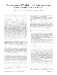
Figure 2-1: A plot of Potential energies vs. separation distance. E1 represents the energy barrier for bubble particle attachment and Hc is the critical rupture thickness of the wetting film.

12

can be used for bubble-particle interactions (Pan and Yoon, 2010). Figure 2-1 shows a plot of all of the surface forces acting between a mineral particle and an air bubble. By using Eq. 26, we obtained the hydrophobic force constant (K131) between two hydrophobic surfaces using the following relation, 𝐾131 = 𝑎𝑒 𝑏𝑘𝜃

[27]

where a and bk are constants which vary with contact angle, θ (Pazhianur and Yoon, 2003). Table 2-1 gives the values of a and bk at different ranges of contact angles. In determining Pa using Eq. 21, we calculated Ek using the following relation, 𝐸𝑘 = 0.5𝑚1 (𝑈𝐻𝑐 ) 2

[28]

where m1 is the mass of the particle, and UHc is the velocity of a particle approaching a bubble at the critical rupture distance (Hc). This velocity may be found by the following relation, 𝑈𝐻𝑐 =

̅1 𝑢

[2]

𝛽

where β is the drag coefficient in the boundary layer of the bubble (Goren and O'Neill, 1971), which in turn can be obtained as follows (Luttrell and Yoon, 1992), 𝑟

0.83

𝛽 = 0.37 ( 𝐻1 )

[30]

which has been derived from the Reynolds lubrication theory. 2.4.2 Probability of Collision Luttrell and Yoon (1992) derived an expression for Pc, which has been modified slightly to ensure that Pc < 1(Do 2010). Eq. (16) above gives an expression for Pc used in the present work. Table 2-1: Values of a and for bk different range of contact angles



a

bk

> 92.28°

6.327x10-27

0.2127

92.28° > θ > 86.89°

4.888x10-44

0.6441

< 86.89°

2.732x10-21

0.04136

13

2.4.3 Probability of Detachment The probability of detachment was calculated using the following expression (Yoon and Mao, 1986), −𝑊𝑎 +𝐸1

𝑃𝑑 = exp (

𝐸𝑘′

)

[31]

where Wa is the work of adhesion, and E’k is the kinetic energy of detachment. Wa can be obtained from the following relation, 𝑊𝑎 = γ𝑙𝑣 π 𝑟12 (1 − cos 𝜃)2

[32]

where γlv is the surface tension of water, r1 is the radius of the particle, and θ is the contact angle. By using Eq.(32), the kinetic energy of detachment (𝐸𝑘′ ) has been calculated using the following relation(Do 2010), 2

𝐸′𝑘 = 0.5𝑚1 ((𝑑1 + 𝑑2 )√𝜀/𝜈)

[33]

where  is the energy dissipation rate and  is the kinematic viscosity. Froth Recovery Model Once particles enter the froth phase, the more hydrophobic particles survive the froth phase and reach the launder while the less hydrophobic particles drop back to the pulp phase. The probability of survival (Rf) is given as (Do, 2010),

𝑑2−0

𝑅𝑓 = 𝑑

2−𝑓

𝑒

−𝑁

2 6ℎ𝑓 𝑑 𝑑 (1− 2−0 )( 1 ) 𝑑2−0 𝑑2−𝑓 𝑑2−0

+ 𝑅𝑤 𝑒

𝜌 −0.0325( 3 −1)−63000𝑑1 𝜌1

[34]

where d2,0 is the diameter of the bubbles entering the froth phase at the bottom, d2,f the bubble diameter at the top, N the number of particles attached to each bubble, hf the froth height, Rw the maximum theoretical water recovery, ρ3 the density of water, and ρ1 is the particle density. The first term of Eq. 34 represents the recovery due to attachment, while the second term represents the recovery due to entrainment (Do 2010). By considering flow balance, one can derive the following relationship,

14

𝑙𝑖𝑞

𝑎𝑖𝑟 ⁄𝑄𝑖𝑛 𝑄𝑜𝑢𝑡 1⁄ −1 𝐸𝑙

𝑅𝑤 =

[35]

𝑙𝑖𝑞 𝑎𝑖𝑟 where 𝑄𝑜𝑢𝑡 is the volumetric flow rate of air leaving the cell, 𝑄𝑖𝑛 the flow rate of pulp entering

the cell, and 𝐸𝑙 is the fraction of water entering a froth launder. The values of these parameters can be readily measured or are readily available in operating plants. Overall Recovery Figure 2-2 shows a mass balance of materials around a flotation cell, in which Rp is the fractional recovery in the pulp phase and Rf is the fractional recovery in the froth phase. As between the pulp and froth zones of a flotation cell. One can readily find that the overall recovery, R, can be calculated using the following relation, 𝑅=𝑅

𝑅𝑝 𝑅𝑓

[36]

𝑝 𝑅𝑓 +1−𝑅𝑝

In a mechanically-agitated flotation cell, the R p can be calculated as follows, 𝑘𝑝 𝑡

𝑅𝑝 = 1+𝑘

[37]

𝑝𝑡

where kp is the flotation rate constant in the pulp phase. Eq. (36) is for perfectly mixed reactor (flotation cell) as is the case with a mechanically-agitated individual cell in a flotation bank. For a plug-flow reactor, Rp can be calculated using the following relation 𝑅𝑝 = 1 − 𝑒 −𝑘𝑝 𝑡

[38]

15

(

-

-

)

PULP (

)

)

1

1-(

FROTH (

(1-

)

)

Figure 2-2: Mass balance of materials around a flotation cell: Rp, pulp recovery; Rf, froth recovery.

Although a laboratory flotation cell is a perfectly mixed rector, Eq. 38 rather than Eq. 37 is used (Levenspiel, 1999), because all of the particles in the cell has the same retention time. For n number of cells, the overall flotation recovery in the bank can be derived using the flowing relation,

𝑅 = 1 − (1 − (𝑅

𝑅𝑝 𝑅𝑓

𝑝 𝑅𝑓 +1−𝑅𝑝

𝑛

))

[3]

if the flotation rate constant remains constant. However, flotation rate constants in the pulp phase hardly remain constant as a feed moves along a bank of lotation cells. For example, the number of floatable particles (N1) changes cell to cell. Therefore, Eq. [39] has not been used in the present work for simulating the performance of flotation banks. The flotation rate constant has been calculated cell to cell as a feed moves along.

16

Chapter 3: MODEL PREDICTIONS The flotation model discussed in the previous chapter is developed from first principles of surface chemistry and hydrodynamics of bubble-particle interactions. The parameters affecting the hydrodynamic properties include particle size, bubble size, energy dissipation rate, etc., while the parameters affecting the surface chemistry are composed of contact angle (θ), zeta-potential, Hamaker constant (A131), and surface tension (γ). Thus, the model can predict flotation recovery and grade from both physical and chemical parameters. In the present work, the flotation feed is represented as a matrix of different particle size and properties such as contact angle, -potential, and degree of liberation. The flotation rate constant (kp), recovery, and grade are then calculated using the flotation model. Standalone Flotation Model Effects of different parameters such as contact angle, particle size, froth height, superficial gas velocity and zeta potential of particle on flotation recovery are studied. Table 3-1 shows the model parameters used for model predictions and simulation. 3.1.1 Contact angle Figure 3-1 shows the effect of contact angle and particle size on the recovery of sphalerite flotation. At a given contact angle, a series of so-called ‘elephant’ curves have been obtained as reported by Trahar and Warren (1976) and Gaudin (1931). The experimental recovery vs. log particle size curves show long tails and sharp nose at the fine and large particle sizes, respectively. The difficulties in floating coarse particles began at particle sizes above 125 µm (100 mesh), while fine particle recoveries decline at 10 µm. The simulation results obtained in the present Table 3-1: Values of the input parameters used in flotation simulation

Variable Specific Power (kW/m3) Superficial Gas Rate (cm/sec) Froth Height (cm) Bubble Zeta Potential (mV) Flotation Time (min) Particle Zeta Potential (mV) Specific Density (sphalerite) Slurry Fraction (%)

Value 1.5 2.0 8 -30 2.5 -15 4.1 10

17

Figure 3-1: Effect of contact angle and particle size on recovery. Input parameters: energy dissipation rate, 1.5 kW/m3; aeration rate, 2 cm/s; S.G. = 3.1, 20 mg/L MIBC; ζ-potential, -15 mV; 2.5 min retention time, 8 cm froth height.

work show also that the problems of floating for both the coarse and fine particles can be overcome by increasing the contact angles of particles. Particle hydrophobicity along with bubble size and particle size represents the three of the most important parameters in flotation. It also shows that the higher the contact angles are, higher the recoveries. Note also that the maximum flotation occurs at the particle sizes in the range of 20 to 105 µm. Eqs.26 and 27 show that hydrophobic force constant for bubble-particle interaction (K132) increases with increasing contact angle. The role of hydrophobic force is to decrease the energy barrier (E1), which in turn causes the probability of bubble-particle attachment (Pa) and hence increase the flotation rate constant (kp) and recovery 3.1.2 Froth height Figure 3-2 shows a contour plot for the changes in recovery with respect to froth height and particle size. It can be seen that the recovery of the coarse particles decreases with increase in the froth height. As the bubble particle aggregates rises through the froth phase in a flotation cell, bubble surface area decreases due to bubble coalescence, which in turn increases the chances of

18

30 90

Froth Height (cm)

25

80 70

20 60 50

15

40 10

30 20

5

10 50

100

150

Particle Size (m)

200

250

300

0

Figure 3-2: Effect of froth height on recovery. Input parameters: energy dissipation rate, 1.5 kW/m3; aeration rate- 2 cm/s; S.G. , 3.1; frother, 20 mg/L MIBC; ζ-potential, -15 mV; 2.5 min retention time, θ =45°.

bubble particle detachment. The froth recovery factor (Rf) decreases more for the coarser particles, hence the overall recovery decreases. 3.1.3 Superficial gas rate Figure 3-3 shows a contour plot for the recovery as functions of superficial gas rate (vg) and particle size (d1). The plot shows that with a rise in the airflow rate, the recovery increased at a given particle size. Many researcher have reported similar results for industrial column flotation in the past (Yianatos, Bergh, and Cortes,1988). 3.1.4 Zeta potential Figure 3-4 shows the effects of particle ζ-potentials and particle size on flotation recovery. As shown in Figure 3-4 Effect of ζ-potential on recovery.

Input parameters: energy dissipation

rate, 1.5 kW/m3; aeration rate- 2 cm/s; S.G. , 3.1; frother, 20 mg/L MIBC; 2.5 min retention time, froth height- 8 cm, θ =45°., fine particle flotation benefits from a decrease in the negative ζpotential of particles, which can be attributed to a decrease in energy barrier (E1) for bubbleparticle interaction. It is well known that the ζ-potential of both air bubbles and mineral particles are negative particularly in sulfide flotation. By reducing the electrostatic repulsion between particles and bubbles, one can reduce the energy barrier for bubble-particle attachment and hence increase the flotation rate. As shown in Eq. (21) a decrease in energy barrier (E1) should increase 19

4

Superficial Gas Rate (cm/sec)

90 3.5

80 70

3

60 2.5

50 40

2 30 1.5

20 10

1 1

10

Particle Size (m)

0

100

 Potential (mV)

Figure 3-3: Effect of superficial gas rate on recovery. Input parameters: energy dissipation rate, 1.5 kW/m3; S.G. , 3.1; frother, 20 mg/L MIBC; ζ-potential, -15 mV; 2.5 min retention time, froth height-8 cm, θ =45°.

-8

80

-10

70

-12

60

-14

50

-16

40

-18

30

-20

20

-22

10

-24 1

10

Particle Size (m)

100

0

Figure 3-4: Effect of ζ-potential on recovery. Input parameters: energy dissipation rate, 1.5 kW/m3; aeration rate- 2 cm/s; S.G. , 3.1; frother, 20 mg/L MIBC; 2.5 min retention time, froth height- 8 cm, θ =45°.

the probability of bubble-particle attachment (Pa) and hence the flotation rate (kp) and recovery. It is interesting that the beneficial effect of controlling the particle ζ-potentials is observed with the flotation of finer particles but not with the coarse particles.

20

Flotation Circuits Simulation In this section effect of circuit arrangement and operating parameters on chalcopyrite recovery was studied. The objective was to be able to generate a recovery versus grade curves which could be used to compare the performance of the different flotation circuits. It was assumed that the contact angle of chalcopyrite feed varies linearly with the feed grade. Table 3-2 shows the operating parameter used for simulation. Circuit arrangement: Three circuits arrangement were considered for the simulation purpose. i)

Rougher Circuit (RC)

F

F

F

C

F

F

C

C T

F

C T

T

C T

C T

T T

C

Figure 3-5: Rougher Circuit

A 6 cell rougher circuit, as shown in Figure 3-5 was studied. Tailings of each preceding flotation cell acted as the feed to the next flotation cell. ii)

Rougher Scavenger Circuits (RSC)

Figure 3-6 shows the rougher-scavenger circuit used for simulation. The circuit comprises of twelve flotation cells. The first six cells act as the rougher, while the next six cells act as the

F

F

F C T

F C

C T

F C

T

T

F

F C T

F C

C T

F

F

C T

F C

C T

T

F C

T

C T

T T

C

Figure 3-6: Rougher scavenger circuit

21

F

F

F C

F

T

F

C

C

C T

T

T

F

F C T

F C

C T

T

F

F

C T

F C

C T

F C

T

C T

T T

F

F

C

F

C T

C T

T

C

Figure 3-7: Rougher scavenger cleaner circuit

scavenger. The rougher tailings were used as feed for the scavenger and the scavenger concentrate was recirculated back to the rougher circuit. iii)

Rougher-Scavenger-Cleaner Circuit (RSCC) Figure 3-7 shows the RSCC with three cleaner cells. The rougher tailing was fed to

the scavenger circuit, while the rougher concentrate acted as the feed to the cleaner circuit. The scavenger concentrate and cleaner tailing were re-circulated to the rougher circuit. 3.2.1 Contact angle The effect of contact angle on floatation recovery of chalcopyrite was studied and the simulation results were plotted for chalcopyrite recovery vs. grade as shown in Figure 3-8. The Table 3-2: Operating parameters for chalcopyrite flotation simulation

Variable

Value

Superficial Gas Rate (cm/sec)

0.5

Froth Height (cm)

20

Contact Angle (chalcopyrite)

60° & 90°

Contact angle (gangue)

5

Particle Zeta Potential (mV)

8

Chalcopyrite Specific Density

4.2

Gangue Specific Density

2.65

22

100

Recovery(%)

80 60

11

6 9m

40 20

Cu = 60

o

Cu = 90

o

3 KW/m 0

0

36 Scv Cln

Rgr

3

10

18

22

20 Grade(%)

30

Figure 3-8: Effect of contact angle on chalcopyrite grade –recovery curve. Input parameters: energy dissipation rate, 3 kW/m3; aeration rate, 0.5 cm/s; θ (Cu) = 60° & 90°; 20 cm froth height; ζ = -8 mV.

dotted lines represent the grade-recovery curve for contact angle of 60º, while the solid line represent the grade recovery curve for 90º contact angle. Numbers above the curves represent the optimum residence times (residence times at the inflection points or ‘shoulders’ of the curves). Specific energy was kept constant at 3kW/m3 for this particular set of simulation. Comparison of the results given in Figure 3-8 show that the RSCC circuit gives a better result than the SC and RSC circuits, which is in agreement to typical industrial practices. It can also be deduced that, with an increase in the contact angle, the circuit performance increases, for all the other parameters being constant. Furthermore, the contact angle increase causes the optimum residence time to decrease, which is an important advantage of using a stronger flotation collector. 3.2.2 Specific energy Effect of changing the specific energy input to flotation was studied by plotting the graderecovery curves. Figure 3-9 shows that an increase in the energy dissipation rate (𝜀̅) from 1 kW/m3 23

100

Recovery (%)

80

60

40

3

Scv

1 kW/m 3 10 kW/m

20

Cln

Rgr

0 0

5

10

15

20

25

30

35

Grade (%) Figure 3-9: Effect of specific energy on chalcopyrite grade –recovery curve. Input parameters: energy dissipation rate, 1 & 10 kW/m3; aeration rate, 0.5 cm/s; θ (Cu)= 90°; 20 cm froth height; ζ =-8 mV.

to 10 kW/m3 resulted in a minor change in grade-recovery curves, but the optimum residence time (residence time at the shoulder of the curve) decreased drastically. Figure 3-10 show the changes in the optimum residence times at 𝜀̅ = 1, 2, 3, 5, 7 and 10 kW/m3. From the plot, it can be observed that with an increase in the energy dissipation rate, the optimum residence time decreases exponentially and becomes steady with further increase in energy dissipation rate. Furthermore, optimum residence time is the highest for the RSCC, followed by RSC and RC, which can be attributed to the larger number of cells in RSCC.

24

Optimum Residence Time (Min)

120 100

Cln

80

Cu = 60

o

Cu = 90

o

60

Scv 40 20 0

Rgr 0

2

4

6

8

10

2

Energy Dissipation(kW/m ) Figure 3-10: Effect of specific energy on optimum residence time. Input parameters: aeration rate, 0.5 cm/s; θ(Cu) = 90° & 60°; 20 cm froth height; ζ =-8 mV.

3.2.3 Froth height The effect of froth height on the grade-recovery curves are shown in the Figure 3-11. The simulation results were obtained assuming that the contact angle of the fully-liberated chalcopyrite particle is 60º. As shown, the grade-recovery curves shift to the upper-right direction, indicating an increase in separation efficiency with increasing froth height. Increment in froth height increases the chance of bubble particle detachment in froth phase, and hence leads to higher selectivity. 3.2.4 Particle Size Figure 3-12 show the grade–recovery curves for the RC circuit for different particle sizes (47µm, 61.8µm, 81.2µm and 106µm). The energy dissipation rate was kept constant at 1 kWm3. The contact angles for the fully-liberated chalcopyrite and gangue mineral particles were assumed

25

100

Recovery (%)

80

60

40

hf= 5 cm

20

Scv

hf= 30 cm 0

Cln

Rgr 0

5

10

15

20

25

30

35

Grade (%) Figure 3-11: Effect of froth height on chalcopyrite grade –recovery curve. Input parameters: energy dissipation rate, 1 kW/m3; aeration rate, 0.5 cm/s; θ(Cu) = 60°; 5 &30 cm froth height; ζ = -8 mV

to be 60º and 5º, respectively. The results show that metallurgical performance increases with decreasing particle size, which can be attributed to the increase in detachment at coarser particles. Figure 3-13 and Figure 3-14 show the same trend between metallurgical performance and particle size for the RSC and RSCC circuits. The ultrafine particles were not considered in this scenario. But if the particle size is less than 20 micron, it might lead to decrement in flotation efficiency due to non-selective entrainment.

26

100

Rougher 47

Recovery(%)

80

61.8 81.2 106 m

60

SiO2 = 5

40

o

Cu = 60

1 KW/m 20

0

o

3

5

10

15

20

Grade(%) Figure 3-12: Effect of particle size on rougher chalcopyrite grade –recovery curve. Input parameters: energy dissipation rate, 1 kW/m3; aeration rate, 0.5 cm/s; θ = 60°; 20 cm froth height; ζ = -8 mV

100

Scavenger

Recovery (%)

47 61.8

80

81.2 106 m 60

SiO2 = 5

o

Cu = 60

1 KW/m 40

0

5

o

3

10

15

20

25

Grade (%) Figure 3-13: Effect of particle size on chalcopyrite grade –recovery curve. Input parameters: energy dissipation rate, 1 kW/m3; aeration rate, 0.5 cm/s; θ = 60°; 20 cm froth height; ζ = -8 mV

27

100

Cleaner

Recovery (%)

47 61.8

80

81.2 106 m 60

SiO2 = 5

o

Cu = 60

1 KW/m 40

0

5

o

3

10

15

20

25

30

35

Grade (%) Figure 3-14: Effect of particle size on chalcopyrite grade –recovery curve. Input parameters: energy dissipation rate, 1 kW/m3; aeration rate, 0.5 cm/s; θ = 60°; 20 cm froth height; ζ = -8 mV

28

Chapter 4: MODEL VALIDATION WITH EXPERIMENTAL DATA Chalcopyrite Batch Flotation Studies were conducted by Muganda et al. (2010) to show the effect of particle size and contact angle on the flotation recovery of chalcopyrite in a series of laboratory-scale batch flotation tests. While specific details of this experiment can be found in the original paper, the test parameters relevant to simulator can be found in Table 4-1. The specific power input (kW/m3) was calculated by assuming a power number of 1.1 and a gassed-to-ungassed power ratio of 0.7. These assumptions are also supported by data elsewhere in the literature (Sawant, 1981). During feed preparation for the batch flotation tests, chalcopyrite was treated in pre-cleaning stages without the addition of collector to reduce the silica to very low levels. In these tests, Muganda et al. conducted flotation tests on pure chalcopyrite samples of different size fractions of known advancing contact angles. For the laboratory tests, the contact angles of different size fractions were manipulated by thermal oxidation and/or conditioning with

100

Maximum Recovery (%)

80

60

40

20

0

Contact Angle 36-40 66-70 71-75

1

10

100

1000

Particle Size (µm)

Figure 4-1: Effect of contact angles on the recovery of pure chalcopyrite particles of different contact angles. Experimental data are from Muganda, et al. (2011), and the curves are from simulation.

29

1.0

Pa

Probability

0.8

1-Pd

0.6

0.4

Pc

0.2

0.0

1

10

100

Particle Size (m) Figure 4-2: Effect of particle size on probabilities (Pa, Pd & Pc); energy dissipation rate, 15 kW/m3; ζ = 77 mV; θ = 35°.

potassium amyl xanthate. The Washburn method was used to measure the advancing contact angles. The flotation tests were conducted at 0.3 cm/s superficial gas rate and 1 cm froth height. Figure 4-1 shows the size-by-size recoveries obtained at three different ranges of contact angles, i.e.,  = 36-40o, 66-70o, and 71-75o. The solid lines represent the results of the simulations carried out using these contact angles, while the points represent the experimental data. Note here that data presented were due to ‘true’ flotation, meaning that the authors subtracted the recoveries due to entrainment from the experimental recoveries. Since Muganda, et al. did not report the values of -potentials, we used the values of -77 mV for minerals and -30 mV for air bubbles. The fit between the Muganda, et al.’s experimental and our simulation results is reasonable. The discrepancies observed at the finer and coarser particle sizes may be due to the possible errors associated in the method of correcting the experimental data for the recovery due to entrainment. The data presented in Figure 4-1 show that the higher the contact angles, the higher the recoveries, and that the optimum flotation occurs at the particle sizes in the range of 20 to 105 µm. 30

1.0

Pa

Probability

0.8

0.6

1-Pd 0.4

0.2

Pc 0.0

10

20

30

40

50

60

70

80

90

Contact Angle  Figure 4-3: Effect of contact angle on probabilities (Pa, Pd & Pc): energy dissipation rate, 15 kW/m3; ζ = 77 mV; Particle size = 20 µm.

An advantage of using a first-principle model for flotation simulation is to analyze the various mechanisms involved. Figure 4-2 shows the probabilities of collision (Pc), attachment (Pa), and detachment (Pd). As shown, both Pa and Pc decreases with particle size, while Pd increases with particle size. Thus, the difficulty in floating fine particles is due to the low collision and attachment probabilities, while the difficulty in floating coarse particles is due to detachment.

Figure 4-3 shows the effect of contact angle () on the probabilities of attachment (Pa), detachment (Pd) and collision (Pc). As shown, Pc is independent of contact angle, while the probability of not being detached, i.e., (1-Pd), increases with , which can be attributed to increasing work of adhesion (Wa) as shown in Eq. [32].

31

1.0

Pa

Probability

0.8

1-Pd

0.6

0.4

0.2

Pc

0.0 10

20

30

40

50

60

70

80

90

Contact Angle 

Figure 4-4: Effect of contact angle on probabilities (Pa, Pd & Pc): energy dissipation rate, 0.5 kW/m3; ζ = -77 mV; Particle size = 20 µm.

Note here that Pa increase with particle size, but the changes are not clearly discernable. The reason for this is because the values of Pa are close to unity at an energy dissipation rate as high as 15 kW/m3. We used this value, because that was the energy dissipation rate employed by Muganda et al. in their laboratory flotation experiments. Figure 4-4 shows the values of Pa, Pc, and 1-Pd obtained using the energy dissipation rate of 0.5 kW/m3. As shown, Pa and 1-Pd are more sensitive to .

32

100

Cumulative Recovery (%)

80

60

40

Dp(µm)



10 63 89

66  77  66



20

0

0

2

4

6

8

10

Flotation Time (mins) Figure 4-5: The effects of contact angles and particle size on the kinetics of flotation. The experimental data were obtained by Muganda, et al. (2011) on pure chalcopyrite samples, and the curves represents the simulation results.

Figure 4-5 describes the effects of contact angle and particle size on the cumulative recoveries of chalcopyrite with the increase in flotation time as reported by Muganda et al. (2010). Table 4-1: Operating parameters used by Muganda et al.

Variable

Value

Rotational Speed (RPM)

1200

Froth Height (cm)

1

Specific Power (kW/m3)

15

Flotation Time (min)

1-8

Superficial Gas Rate (cm/s)

0.3

Cell Volume (L)

5

Cell Area (m2)

0.04

Frother Type

PPG 33

The lines represent the simulation results, while the points represent the experimental recoveries. A reasonably good fit can be seen between the experimental and simulation results. Batch Silica Flotation Closely controlled laboratory flotation tests were performed on mono-sized glass beads to validate the simulator outcome over various feed properties and operating conditions. Flotation experiments were conducted on mono-sized glass beads using a 1.2 liter laboratory scale Denver flotation machine. The particle sizes of the beads were in the range of 35 to 119 µm. Dodecylamine hydrochloride (DAH) was used as collector while MIBC was added as frother. To maintain a uniformity in all laboratory tests, a 4 x 10-6 M DAH-in-ethanol solution was prepared as a stock solution. A known volume of the stock solution was used in flotation and contact angle measurement. Table 4-2 summarizes the flotation conditions. For contact angle measurements, a clean and polished glass plate was conditioned in the solution for two minutes prior to the measurements. The standard goniometer-based on sessile drop technique was used for all the contact angle measurements. The process involved vertical dropping of a water droplet on to the surface of the prepared silica plate. The surface was then captured by high resolution camera and then analyzed using Ramé–hart Model 250. To ensure the correct measurement of contact angles, each measurement was repeated five times on each glass plate and the average value for the contact angle was calculated. In flotation tests, regulated pressurized air was introduced to a flotation cell through the impeller shaft and rotor and the superficial gas rate was monitored by means of a flow meter (GFM, Aalborg make). Table 4-2: Operating parameters for silica batch flotation experiments

Variable

Value

Rotational Speed (RPM)

850

Froth Height (cm)

1.5

Specific Power (kW/m3)

2.71

Flotation Time (min)

0.5 - 4

Superficial Gas Rate (cm/s)

1

Cell Volume (L)

1.2

Frother Type

MIBC

34

A known quantity (120 g) of glass beads was added to the 1.2 liter Devner flotation cell and agitated for 30 seconds in the presence of MIBC and DAH. The agitation was stopped and the pH was measured, after which the slurry was agitated again for another 1 minute without air. After the 1 minute conditioning time, air was introduced to commence flotation. Each flotation experiment lasted for 4 minutes, during which time a set of five samples were collected. The first three sample were collected at interval of 30 seconds, followed by two progressively long intervals (1min and 1.5 min). The collected flotation products were dried in an oven and weighed. From the weight, flotation recoveries were calculated. The results were plotted as a function of time to obtain kinetic information. Effect of particle size on silica flotation recovery is shown in Figure 4-6. Laboratory scale flotation tests were conducted on pure glass spheres of different particle size (35, 71 and 119 µm). The flotation test were conducted at 1cm/s superficial gas rate, 1.5 cm of froth height, and 2.5 kW/m3 energy dissipation rate. The solid line represents the simulation results while the points represents the experimental cumulative recoveries. The experimental data fit reasonably well with the simulations result.

100

119 71

Cumulative Recovery (%)

80 35 60

40  = 51



kW/m

20

0

3

Vg = 1 cm/s Froth Height = 1.5 cm

0

1

2 Flotation Time (min)

3

4

Figure 4-6: Effect of particle size on the kinetics of silica flotation.

35

100 9.71 (1300)

80

6.72 (1150)

Recovery (%)

2.71 kW/m (850 RPM)

60

S.G. = 2.5

40

 = 38



Vg = 1 cm/s d1= 35 m

20

Froth Height = 1.5 cm 0

0

1

2

3

4

Time (min)

Figure 4-7: Effects of energy dissipation on the kinetics of silica flotation: particle size, 35 µm.

Figure 4-7 shows the effect of specific energy input on the recovery of silica particles. In these experiments, 35 µm silica particles were used, with the Denver flotation machine operating at 850, 1150 and 1300 RPM. As shown, the flotation kinetics and hence the recovery increases with increasing energy input. Note here that the simulation results are in reasonable agreements with the experimental dada, validating the first-principle model and the simulation results obtained in the present work. Figure 4-8 shows that the values of Pa, Pc, and Pd as calculated using the model under the experimental conditions employed in the flotation experiments. As shown, both Pa and Pc increased with increasing energy dissipation rate (𝜀̅), while the probability of not being detached (1-Pd) increases with 𝜀̅. The flotation recovery increased with increasing energy input shows that the detrimental impact of particle detachment is overcome by the beneficial effects of Pa and Pc.

36

1.0

Pa

Probability

0.8

0.6

0.4

1-Pd

0.2

Pc 0.0

0

2

4

6

8

10

3

Specific Power (kW/m ) Figure 4-8: Effect of specific energy on probabilities (Pa, Pd & Pc): Particle size = 35 µm; θ = 38°.

Figure 4-9 shows the effects of contact angle () on the recovery of the 35 µm silica particles. The hydrophobicity of the particles were controlled by varying the DAH dosages. As expected, the recoveries increased with the increase in the hydrophobicity. As discussed earlier, an increase in particle hydrophobicity helps in reduce the energy barrier (E1) for bubble-particle interaction, which in turn increases Pa. The increase in  also increases the work of adhesion (Wa), and hence decreases Pd. The results presented in Figure 4-9 show that there are reasonable agreements between the experiment and simulation, validating the first-principle model developed in the present work.

37

100   = 61

Cumulative Recovery (%)

80



51

 

60

40

S.G. = 2.5 2.5 kW/m

3

Vg = 1 cm/s d1= 35 m

20

Froth Height = 1.5 cm 0

0

1

2

3

4

Flotation Time (min) Figure 4-9: The effects of contact angle on the kinetics of silica flotation: particle size, 35 µm.

Selective Flotation In another set of flotation tests were carried out on a mixed feed consisting of 10% silica (SiO2) and 90% magnetite (Fe3O4) by weight. The glass beads were mono-sized particles with a designated size of 75 µm, while that of magnetite was a -75+53 µm fraction. The latter sample was obtained from the Alpha Chemicals. The glass beads were cleaned in a Piranha solution at 70ºC in order to remove all the contamination. The particles were then rinsed three to four times with ultrapure water in an ultrasonic bath. The glass beads were then dried in an oven. The dried samples were then immersed in a freshly prepared 2x10−5 M octadecyltrichlorosilane (OTS)-in-toluene solution for a given period time. A glass slide was immersed in the same solution so that the contact angles of the glass beads and glass slide were the same. After the immersion, the excess OTS was removed from the silylated surfaces by quickly washing the plates and particles sequentially with chloroform, acetone and pure water. After the excess OTS had been removed, the silylated plates 38

were blow-dried using a stream of pure nitrogen. The hydrophobicity was controlled by controlling the time of contact between the glass spheres and OTS solution. The equilibrium, advancing, and receding contact angles were determined using the sessile drop technique by means of a contact angle goniometer. With a given silica plate, the measurements were repeated five times and averaged. The flotation tests were carried out on the 1:9 mixtures of hydrophobized silica and magnetite particles using the Denver laboratory flotation machine with a 1.2 liter flotation cell. In each test, 120 grams of the mixture and MIBC were added to the cell and conditioned for 30 seconds. After the agitation, the pH of solution was measured. The slurry was agitated further for another minute without air, after which a regulated air flow was introduced to commence the flotation test for a total of 4 minutes. Five samples were collected. The first three samples were collected at intervals of 30 seconds, followed by two progressively longer intervals (1 min and 1.5 min). The flotation recoveries were determined from the timed weights of the froth products. The results were plotted as a function of time in order to produce standard kinetic curves. Both the flotation concentrate and tails were subjected to magnetic separation to determine the product grades. The first set of flotation tests were conducted by varying the impeller speed in the range of 850, 1,050 and 1,300 RPM, while keeping all other variables constant. Figure 4-10 shows the effects of the RPM, or energy dissipation rate (𝜀̅), on the recovery of silica and magnetite. As shown, silica floated much faster than magnetite because the former was hydrophobic. The silica samples were hydrophobized in a 2x10−5 M OTS-in-toluene solution for 30 seconds to obtain an equilibrium contact angle of 61o. Note here that the increase in 𝜀̅ does not change the recovery of the hydrophobic silica. However, the recovery of the hydrophilic magnetite increased with increasing𝜀̅. The net result is that the grade of froth product decreased with increasing 𝜀̅. Figure 4-11 shows the grade-recovery curves in the flotation experiments. Also shown in the figure are the simulated grade-recovery curves. The experimental results obtained at the lower energy dissipation rates are lower than the simulated, while the results obtained at the higher dissipation rates show an excellent agreement. The discrepancy observed at the lower energy dissipation rates may be due to the possibility that the silica-magnetite mixtures were not fully suspended.

39

100 Silica

Recovery (%)

80

3

2.71 kW/m 3 5.12 kW/m 9.71 kW/m

60

40 Magnetite

20

0

4

3

2

1

0

Flotation Time (min) Figure 4-10: The effects of specific energy on the kinetics of silica and magnetite flotation: energy dissipation rate, 2.71 kW/m3; aeration rate, 1 cm/s; 1.5 cm froth height; θsilica = 62°, θmag= 7°.

100

95

Recovery (%)

90

85

80 3

2.71 kW/m 3 5.12 kW/m 3 9.71 kW/m

75

70 30

40

50

60

70

80

90

100

Grade (%)

Figure 4-11: The effects of specific energy on the grade as a function of recovery: energy dissipation rate, 2.71 kW/m3; aeration rate, 1 cm/s; 1.5 cm froth height; θsilica = 62°, θmag= 7°.

40

Figure 4-12 shows a set of selective flotation tests conducted on the 1:9 hydrophobic silicahydrophilic magnetite mixed particle suspension by varying the superficial gas rate. The equilibrium contact angle of the silica was 63º after 30 seconds of contact time with a 2x10−5 M OTS-in-toluene solution. As expected, the silica recoveries were higher at 1.0 cm/sec gas rate than at 0.5 cm/s gas rate. Similar results were reported by Yang and Aldrich (2006). The solid lines show the simulation results obtained assuming that the magnetite contact angle was 7o. Reasonable agreements were obtained at the longer flotation time. At the shorter flotation times, the simulated results were lower than the experimental results. Figure 4-13 shows the grade vs. recovery curves obtained on the basis of the data presented in Figure 4-12. The simulated and predicted results are in reasonable agreement.

100 Silica

Recovery (%)

80

60 0.5 cm/s 1.0 cm/s 40

20 Magnetite

0

0

1

2

3

4

Flotation Time (min) Figure 4-12: The effects of superficial gas rate on the kinetics of silica and magnetite flotation: energy dissipation rate, 2.71 kW/m3; aeration rate, 1 cm/s; 1.5 cm froth height; θsilica = 64°, θmag= 7°.

41

100

95

Recovery (%)

90

85

80

0.5 cm/s 1.0 cm/s

75

70 40

50

60

70

80

90

100

Grade (%)

Figure 4-13: The effects of superficial gas rate on the grade as a function of recovery: energy dissipation rate, 2.71 kW/m3; aeration rate, 1 cm/s; 1.5 cm froth height; θsilica = 64°, θmag= 7°.

100 Silica

Recovery (%)

80

60   = 52

40

  = 61

20

0

Magnetite

0

1

2

3

4

Flotation Time (min) Figure 4-14: The effects of contact angle on on the kinetics of silica and magnetite flotation: energy dissipation rate, 2.71 kW/m3; aeration rate, 1 cm/s; 1.5 cm froth height; θmag= 7°.

42

Figure 4-14 shows the results of two sets of flotation tests conducted on the 1:9 mixtures of hydrophobic silica and hydrophilic magnetite. In one test, the silca sample had a contact angle of 51o and in the other the contact angle as 61o. As has already been noted, the contact angle was controlled by controlling the immersion time in a 2x10-5 M OTS-in-toluene solution. As expected, hydrophobic silica particles floated much faster than the hydrophilic magnetite. Also, the recoveries of the silica particles with  = 61o were higher than those of the silica with  = 52o. It is interesting to find that the magnetite particles floated better in the presence of the less hydrophobic particles. This finding may be explained by the likelihood that the magnetite particles may have a lesser competition with the silica particles when the latter is less hydrophobic. This phenomenon has not been reflected in the model development. Therefore, the simulation did not fit the experimental data well. For this reason, no simulation results are presented in Figure 4-14.

43

Chapter 5: CONCLUSION General Conclusion Flotation models are an important tool to develop better understanding of the flotation process. The first-principle model developed in the present work can be used to evaluate the performance of a flotation machine or flotation circuit without the need of extensive laboratory experiments. A unique advantage of the model/simulator developed in the present work is that for the first time one can predict flotation results from both the hydrodynamic and chemistry parameters. The model has been validated from a series of carefully controlled flotation experiments. Further, the simulation results presented in this communication are consistent with the flotation practice. Recommendations for Future Work While the simulation shows reasonable fit with the experimental data, they may not be sufficient. Model is made of some assumptions and simplification, which could be improved while considering following suggestions

Include an analytical expression for bubble coarsening in the froth (or foam) phase.



Include a model to predict the contact angle of particle based on liberation analysis.



Incorporate the effect of hydrophobic coagulation.



Develop the model to relate zeta-potential with pH and contact angle with dosages with collector dosages.



Take effect of presence of other particles of different species on bubble coverage.

44

REFERENCES Abrahamson, J, 1975. Collision rates of small particles in a vigorously turbulent fluid, Chem. Eng. Sci., 30, 1371-1379. Ahmed, N and Jameson, G J, 1985. The effect of bubble size on the rate of flotation of fine particles, Int. J. Miner. Process., 14: 195-215. Ata, S, Ahmed, N, Jameson G J, 2002. Collection of hydrophobic particles in the froth phase, Int. J. Miner. Process., 64, pp. 101–122. Brewis, T., 1996. Flotation cells. Mining Magazine, 160(7): 18–24. Do, H, 2010. Development of a Turbulent Flotation Model from First Principles, PhD Dissertation, Virginia Polytechnic Institute and State University, Blacksburg, VA. Fuerstenau, D W, 2007. A century of developments in the chemistry of flotation processing, Froth Flotation: A Century of Innovation, SME, Denver, CO, USA, pp. 1–13. Fuerstenau, D W, Fine particle flotation, P Somasundaran (Ed.), 1980. Fine Particles Processing, AIME/SME, New York, pp. 669–705. Goren, S L and O'Neill, M E, 1971. On the hydrodynamic resistance to a particle of a dilute suspension when in the neighbourhood of a large obstacle, Chem. Eng. Sci., 26: 325338. Hogg, R, Healy, T W, and Fuerstenau, D W, 1966. Mutual coagulation of colloidal dispersions, Transactions of Faraday Society, 62:1638-1651. Kelsall, D. F. (1961). Application of probability assessment of flotation systems. Transactions of the Institution of Mining and Metallurgy, 70(3), 191-204. Lee, C A., Erickson, L E, 1987. Bubble breakup and coalescence in turbulent gas-liquid, Chem. Eng. Commun., 59:65-84. Levenspiel O, 1999. Chemical Reaction Engineering, third edition, John Wiley & Sons, New York, USA, pp. 90-112. Luttrell, G H., Yoon, R-H, 1992. A Hydrodynamic Model for Bubble-Particle Attachment, J. Colloid Interface Sci., 154:129-137. Lynch, A J, Watt, J S, Finch, J A, Harbort, G J, 2007. History of Flotation Technology. Froth Flotation: A Century of Innovation, SME, Denver, CO, USA, pp. 1–15 Moys, M H, 1978. A study of a plug flow model for flotation froth behavior,Int. J. Miner. Process., 5, pp. 221–238 45

Muganda, S, Zanin, M., Grano, S R, 2011. Influence of particle size and contact angle on the flotation of chalcopyrite in a laboratory batch flotation cell, Int. J. Miner. Process., 98(3-4):150-162. Pan, L., Yoon, R-H, 2010. Hydrophobic Forces in Wetting Films, Faraday Discuss., 146:325340. Pan, L, Jung, S., Yoon, R-H, 2011. A fundamental study on the role of collector in the kinetics of bubble–particle interaction, J. Colloid Interface Sci., 361(1):321-330. Pan, L, Jung, S., Yoon, R-H, 2012. Effect of Hydrophobicity on the Stability of the Wetting Films of Water Formed on Gold Surfaces, Int. J. Miner. Process., 106-109:37-41. Pazhianur, R., Yoon, R-H, 2003. Model for the origin of hydrophobic force, Miner. Metall. Process, 20:178-184. Rabinovich, Y., Churaev, N V, 1979. Effect of electromagnetic delay on the forces of molecular attraction, Kolloidn Zh, 41:468-474. Savassi, O.N., 1998. Direct estimation of the degree of entrainment and the froth recovery of attached particles in industrial flotation cells. Ph.D. Thesis, The University of Queensland, Australia. Schubert, H, 1999. On the turbulence-controlled microprocesses in flotation machines, Int. J. Miner. Process., 56:257-276. Schultz, C W, Mehta, R K, Bates, J B, 1991. The flotation column as a froth separator, SME Annual Meeting, Denver, CO Schulze, H J, 1984. Physico-chemical Elementary Processes in Flotation. (Elsevier. New York) Sherrell, I., Yoon, R-H, 2005. Development of a Turbulent Flotation Model, in Proceedings of the Centenary of Flotation Symposium, pp 611. Sutherland, K L, 1948. Kinetics of the flotation process, J. Phys. Chem., 52:394-425. Sutherland, D N, 1989. Batch Flotation Behaviour of Composite Particles, Miner. Eng., 2:351367. Trahar, W J and Warren L J, 1976. The flotability of very fine particles - A review, Int. J. Miner. Process., 3(2):103-131. Tomlison, H S and Fleming, M G, 1963. Flotation rate studies, in Mineral Processing. Congr. of Miner. Process., (ed: A Roberts) pp 563-579 (Pergamon Press, New York).

46

Villeneuve J, Guillaneau J C, Durnace M V, Flotation modelling: A wide range of solutions for solving industrial problems, Minerals Engineering, 8 (4/5) (1995), pp. 409–420 Warren, L, J, Determination of the contribution of true flotation and entrainment in batch flotation tests Int. J. Min. Process., 14 (1985), pp. 33–44. Yang, Y, Ma, J, Jung, S and Yoon, R-H, Dynamics of Bubble-particle Interaction, in Separation Technologies for Minerals, Coal, and Earth Resources, (ed: C A Young and G H Luttrell) pp 27-34 (Society for mining, metallurgy, and exploration, Inc., Colorado) Xu. Z and Yoon, R H, 1989. The Role of Hydrophobic Interactions in Coagulation, J. Colloid Interface Sci., 132(2):532-541. Yoon, R-H and Aksoy B S, 1999. Hydrophobic Forces in Thin Water Films Stabilized by Dodecylammonium Chloride, J. Colloid Interface Sci., 211:1-10. Yoon, R-H. and Luttrell, G H, 1989. The effect of bubble size on fine particle flotation. Miner. Process. Extract. Metall. Rev. 5, 101-122. Yoon, R-H and Mao, L, 1996. Application of Extended DLVO Theory, IV: Derivation of Flotation Rate Equation from First Principles. J. Colloid Interface Sci., 181:613-626. Yoon, R-H and Ravishankar, S A, 1994. Application of Extended DLVO Theory: III. Effect of Octanol on the Long-Range Hydrophobic Forces between Dodecylamine-Coated Mica Surfaces, J. Colloid Interface Sci., 166(1):215-224. Yoon, R-H, Flinn, D H and Rabinovich, Y I, 1997. Hydrophobic Interactions between Dissimilar Surfaces. J. Colloid Interface Sci., 185:363-370. Yoon, R-H and Wang, L, 2006. Hydrophobic Forces in Foam Films, in Colloid Stability -The Role of Surface Forces, Colloid and Interface Science Series, (ed: T F Tadros), pp 161186(Wiley-VCH). Young, J., 1982. Tec Systems - Flotation Drying for the Converting, Paper, and Process Industries. Tappi Journal, 65(11): 46-49.

47