classification indices were proposed for all types of cup anemometers. As a re- sult of the classification, the cup anemometer will be assigned to a certain class:.
Risø-R-1348(EN)
Development of a Classification System for Cup Anemometers CLASSCUP Troels Friis Pedersen
Risø National Laboratory, Roskilde April 2003
Abstract Errors associated with the measurements of the wind speed are the major sources of uncertainties in power performance testing of wind turbines. Field comparisons of well-calibrated anemometers show a significant and not acceptable difference. The European CLASSCUP research project posed the objectives to quantify the errors associated with the use of cup anemometers, and to determine the requirements for an optimum design of a cup anemometer, and to develop a classification system for quantification of systematic errors of cup anemometers. The present report describes this proposed classification system. A classification method for cup anemometers has been developed, which proposes general external operational ranges to be used. A normal category range connected to ideal sites of the IEC power performance standard was made, and another extended category range for complex terrain was proposed. General classification indices were proposed for all types of cup anemometers. As a result of the classification, the cup anemometer will be assigned to a certain class: 0.5, 1, 2, 3 or 5 with corresponding intrinsic errors (%) as a vector instrument (3D) or as a horizontal instrument (2D). The classification of three commercial cup anemometers showed that for the normal category, the best class for horizontal wind speed measurements was class 2 and for vector measurements class 3. The CLASSCUP prototype anemometer got a class 2 as a horizontal anemometer and class 1 as a vector anemometer. For the extended category the commercial cup anemometers were class 5 both for horizontal and vector measurements, whereas the CLASSCUP anemometer got a class 3 as a vector instrument.
ISBN 87-550-3076-9 ISBN 87-550-3075-0 (Internet) ISSN 0106-2840 Print: Pitney Bowes Management Services A/S, 2003
Contents Preface 4 1.
Introduction 5
2.
External Conditions for Classification of Cup Anemometers 6
2.1 2.2 2.3 2.4 2.5 2.6 2.7 2.8 2.9
Classification Principles 6 External Operational Conditions 6 Wind speed range 7 Turbulence intensity ranges 7 Spectrum length scales 8 Air temperature ranges 9 Air density range 10 Slope of terrain ranges 10 Summary of operational limits 10
3.
Classification Procedure 12
3.1 Classification index 12 3.2 Defining the Measurand 12 3.3 Laboratory and Wind Tunnel Tests 13 3.4 Time Domain Modeling of Cup-Anemometers 14 3.4.1The Drag Coefficient Model 16 3.4.2The Parabolic Torque Coefficient Model 20 3.4.3The torque coefficient model with wobbles 23 3.4.4CQ table interpolation 26 4.
Classification Examples 28
4.1 Cup anemometer data 30 4.2 Classification 32 5.
Conclusions 43
6.
References 44
Risø-R-1348(EN)
3
Preface The following report is the result of the development of a classification system of cup anemometers. The work was made in the European CLASSCUP research project under contract with the European Commission, project number JOR3CT98-0263. Additional support to the project was given by the Danish Energy Agency under the Renewable Energy Development programme with the contract number 51171/98-0016.
4
Risø-R-1348(EN)
1. Introduction Very accurate measurements of the wind speed are essential to the wind energy community. This is a fact for measurements of wind resources, which determines the overall driving economics of wind energy. But it is even more true for measurements of the power performance of wind turbines, on which manufacturers sell their wind turbines and for which contractual agreements determine whether the individual wind turbines are able to perform satisfactory or not. In the latter case, the wind speed measurement is the most important single contribution to the uncertainty of the power performance measurement. The wind speed sensors are therefore, by no discussion, the most important instruments to the wind energy community. So far, cup-anemometers have been dominating in wind energy applications. They are being used predominantly in wind energy assessments, and they are at present the only instruments being accepted in power performance measurements in international standards. The reason why the cup-anemometer is so successful is the simple construction, the low price, and yet very good characteristics. A variety of cup-anemometers are available on the market. Sizes, cup shapes, body shapes and dimensions vary significantly on different designs. A number of investigations have been made to evaluate cup-anemometers for wind energy applications. The problem is, that the selection criteria for the specific applications need to be based on adequately detailed investigations of each specific cup-anemometer design. Despite the efforts so far, it is still a difficult task to set up objective criteria to classify cup-anemometers for given purposes. This report will be focusing on a procedure to evaluate cup anemometers. The basis for the evaluation is laboratory and wind tunnel tests, which are made under well-controlled conditions. The systematic errors are evaluated for specific ranges of environmental operational conditions, which refer to certain use of a cup anemometer. For such well-defined purposes, cup anemometers are related to a classification scheme, which can be directly used in uncertainty estimates. The report on the proposed classification system for cup anemometers was part of a European research project, CLASSCUP, Ref. 1.
Risø-R-1348(EN)
5
2. External Conditions for Cup Anemometer Classification 2.1
Classification Principles
A standard for classification of cup anemometers shall make it easy to select cup-anemometers for wind speed measurements. Selection of power converters is very easy due to such a classification system for electric monitoring equipment. The classification of electric power converters is based on requirements of accuracy of the instruments being lower than a certain level (classification level) for well-defined operational ranges. In specifying the power measurement equipment for a power performance test of a wind turbine, the test engineer should look at whether the claimed uncertainty classification of the measurement equipment, particularly the current and voltage transformers and the power transducer, can be retained. Given the nature of the measurands, i.e. the expected currents and voltages, the effect on the related variables should be critically analysed. The International Electrotechnical Commission has published class indices for power monitoring and related equipment. Power transducers are covered by IEC 60688: 1992, Ref. 2, voltage transformers by IEC 60044-2:1997, Ref. 3 and current transformers IEC 60044-1:1996, Ref. 4. In the case of a power transducer a classification of 0.1, 0.2, 0.5 or 1 indicates that the limits of intrinsic error will be within ±0.1%, ±0.2%, ±0.5% or ±1.0% where the ‘feduciary’ value is the span. In the case of current and voltage transformers, similar classifications apply. In order to provide a classification system of cup anemometers similar to the classification system of electric measuring devices, the external operational conditions shall be well-defined and operational limits for the classification shall be set up.
2.2
External Operational Conditions
Typical power curve measurements at “ideal” sites do not require very hard operational requirements for cup anemometers, whereas power curve measurements at complex terrain site requirements are somewhat stronger. It seems therefore necessary to make two classification categories. A first category should relate to “ideal” sites, which will be called a normal category. The second category should relate to more complex sites, and is called an extended category. The environmental operational ranges of the wind itself, which influences the operation of the cup anemometer, are the turbulent wind itself, the air temperature and the air density. The three-dimensional turbulent wind spectra are very site specific, but we are interested in covering specific purposes, which can be represented by general formulations of wind spectra. The Kaimal spectrum, as described in the IEC Wind Turbine safety standard, Ref. 5, can be used as the
6
Risø-R-1348(EN)
basis for the description. For wind energy purposes, the lowest levels near the ground with very low longitudinal length scales are not the most relevant for large wind turbines, and not even for small wind turbines, which are often raised above tree level. These low levels would be more demanding for cup anemometers in the high frequency range. The longitudinal Kaimal spectra is modelled by:
fS k ( f )
σ
2 k
=
4 fLk / V (1 + 6 fLk / V ) 5 3
The average wind speed V, the standard deviation σk and the length scale Lk are descriptive parameters for which their ranges must be determined. The IEC standard for power performance measurements, Ref. 6, considers the applicability of the terrain and divides terrain into two categories. The first category, called “ideal” terrain, considers reasonably flat terrain with rather small slopes. The second category is terrain, which do not meet the requirements of the ideal terrain. In this category, complex terrain with steep slopes is included.
2.3
Wind speed range
Most wind speed measurements in wind energy applications are related to wind resource and wind utilisation purposes. For these purposes 10 minute averages are used. Below 4 m/s the power in the wind is insignificant and above 16 m/s, the power from the wind turbine is regulated to be almost constant and independent of the wind speed. At 25 m/s the wind turbines are normally stopped. For wind energy related applications 4-16 m/s is the range in which the wind speed must be measured with a very high accuracy. This is also the wind speed range being used in calibration of cup anemometers in the MEASNET calibration procedure, Ref. 7. The range 4-16m/s is therefore selected for cupanemometer classification purposes for the classification categories.
2.4
Turbulence intensity ranges
The IEC safety standard, Ref. 5, gives guidance as to the relevant range of turbulence intensities. The maximum standard deviation of the wind speed for a given confidence level of probability is expressed in a formula. For a 95% confidence level and for high turbulence (Ref. 5, case A) we have I15=0,18 and a=2:
σ 1 = 1,13m / s + 0,12Vhub ⇒ Ti =
1,13m / s + 0,12 Vhub
The 95% confidence level is chosen for the extended range. For the normal range, the 90% confidence level is chosen:
σ 1 = 0.48m / s + 0,12Vhub ⇒ Ti =
Risø-R-1348(EN)
0,48m / s + 0,12 Vhub
7
Completely constant wind speeds are never seen. The lowest turbulence intensities that are considered to be relevant are 3% at all wind speeds. Figure 2-1 shows the selected turbulence intensity levels for normal and extended ranges. Turbulence ranges for Normal and Extended Categories 45
Turbulence intensity [%]
40 Max Normal Max Extended Min Both
35 30 25 20 15 10 5 0 0
2
4
6
8
10
12
14
16
18
Wind speed [m/s]
Figure 2-1 Turbulence intensity ranges as function of wind speed for normal and extended categories
2.5
Spectrum length scales
The average length scale of the longitudinal spectrum is varying over a broad spectrum. For a specific site at Vindeby, Ref. 8, the longitudinal length scales have been analysed for both onshore (LM) and offshore positions (SMS and SMW), as shown in Fig. 2-2. The dashed curves are at 3m height.
8
Risø-R-1348(EN)
Figure 2-2 Longitudinal length scales measured onshore and offshore at Vindeby, from Ref. 8. For both positions the average longitudinal length scales seem to be constant at about 500m except for the 3m height. From the plots, a good range of length scales is seen to be from 100m up to 2000m. The ratios of the standard deviations of the three wind speed components, σu:σv:σw, are generally in flat terrain found to be 1:0.8:0.5, Ref. 9. For complex terrain, the turbulence structure can be regarded isotropic, with the ratios 1:1:1, Ref. 9. These ratios are selected to correspond to normal and extended categories, respectively.
2.6
Air temperature ranges
The environmental air temperature is the temperature to which the cupanemometer is exposed, but not necessarily the temperature of the bearings, which might be heated in several types of cup-anemometers. The air temperature ranges of operational wind turbines are according to the IEC safety code, Ref. 5, -10° to 40° for normal conditions and -20° to 50° for extreme conditions. In order to measure very accurate power curves under the normal category, it is
Risø-R-1348(EN)
9
necessary not to include temperatures at which cup anemometer are exposed to rime, snow and ice. For this reason, it seems reasonable to select a temperature range for the normal category from 0° to 40°, and -10° to 40° for the extended category. For an arctic category, the full temperature range from -50° to 50° could be used, and rime, snow and icing conditions should be taken into account. Such arctic conditions are not at all considered in this report.
2.7
Air density range
The air density is affecting the ratio of frictional forces to the aerodynamic forces. For altitudes up to 2000m the standard air density ranges from 1,225 to 1,006 kg/m3, according to ISO Standard Atmosphere, Ref. 10. For a constant altitude an air density range of about ±10% is assumed. On this basis a total air density range of 0,900 to 1,350 kg/m3 would be reasonable. The air humidity variations are assumed included in the air density range, and are assumed otherwise not to affect the operation of cup-anemometers.
2.8
Slope of terrain ranges
The slope of the terrain may change the wind vector components. Wind turbine sites and power performance measurements are performed also in mountainous terrain where the slope of the terrain might be high. The inflow to the cupanemometer might thus be constantly skew. To cover the most applications, but not all extreme cases, a range of flow slopes of -15° to 15° should be used for an extended range. The accepted average slope of terrain in the IEC power performance document, Ref. 6, is 3°, but 5° slope of the flow would in such a terrain be within the common range. A range of flow slopes of -5° to 5° is therefore selected for the normal category.
2.9
Summary of operational limits
The following tables show the operational ranges of the proposed classification categories.
10
Risø-R-1348(EN)
Table 2-1 Normal Range (Typical operational ranges for wind turbine power performance measurements at ideal sites) Parameter Wsp (10min) [m/s] Turb.int. Turbulence structure σu/σv/σw. Length scale Lk [m] Air temp. [°C] Air density [kg/m3] Slope [°] Ice, snow, rime conditions
Min 4 0.03
100 0 0.9 -5
Normal range Ave Max 4-16 16 0.10 0.12+0.48/V 1/0.8/0.5 500 10 1.23 0
2000 40 1.35 5
not included
Table 2-2 Extended Range (Typical operational ranges for wind turbine power performance verification measurements including complex terrain) Parameter Wsp (10min) [m/s] Turb.int. Turbulence structure σu/σv/σw. Length scale Lk [m] Air temp. [°C] Air density [kg/m3] Slope [°] Ice, snow, rime conditions
Min 4 0.03
100 -10 0.9 -15
Extended range Ave Max 4-16 16 0.10 0.12+1.13/V 1/1/1 500 10 1.23 0
2000 40 1.35 15
excluded
The two categories are specifically not considering arctic conditions, and are avoiding the special problems under such conditions.
Risø-R-1348(EN)
11
3. Classification Procedure 3.1
Classification index
The class index system is based on systematic variations of the output signal due to variations in influence quantities. The influence quantities are: air temperature, air density, turbulence intensity and average slope of terrain or flow angle. For cup anemometers the relevant class indices would not be ranging over decades. Therefore it is proposed to keep the indices mostly on a proportional scale, as shown in Fig. 2-3. The ranges shall not be expressed totally as percentages or totally as absolute values. In these cases it would the systematic errors in the lower wind speed range or high wind speed range, respectively, that would dominate the classification. The compromise is an index range, which combines the absolute and the relative deviations: Range=± IndexClass*(0.1m/s+0.01*U)/2
Permissible Deviations [m/s]
Permissible Limits of Error for Cup Anemometer Class Indices 0,8 0,7 0,6 0,5 0,4 0,3 0,2 0,1 0 -0,1 -0,2 -0,3 -0,4 -0,5 -0,6 -0,7 -0,8
Class 0.5 Class 1 Class 2 Class 3 Class 5
0
2
4
6
8
10
12
14
16
18
20
Wind Speed [m/s]
Figure 3-1, Proposed class indices for cup anemometers
3.2
Defining the Measurand
The measured wind speed of a cup anemometer is an averaged one-dimensional quantity. The interpretation of this quantity, though, is important in order to make a consistent classification. Considering a time dependent 3D wind speed vector with a longitudinal component u, a transversal component v, and a vertical component w as input to the cupanemometer.
G U = (u, v, w )
12
Risø-R-1348(EN)
The measured wind speed of a cup anemometer, the measurand, is in this report defined in two different ways. The most often considered definition of measured wind speed of a cup anemometer is the “horizontal” wind speed. This definition measures only the horizontal wind speed components (length of the wind speed vector, excluding the vertical component):
G U = ∫ u2 + v2 t
If the cup anemometer has a cosine angular response, the vertical component w automatically is filtered away, and it covers the “horizontal” wind speed definition, which also could be called a 2D averaged measurement. The second definition includes the vertical component w. It has been called a “vector” measurement, though it only measures one parameter. On the other hand it includes all the three vector components, so it is a 3D averaged measurement.
G U = ∫ u 2 + v 2 + w2 t
The difference between these two definitions is dependent on the turbulence intensity. For 15% turbulence in a flat terrain, the difference is about 0.5%, and for 30% turbulence it is about 1%. This is not significant, but it is enough to distinguish between the two definitions in a classification procedure.
3.3
Laboratory and Wind Tunnel Tests
Testing of cup anemometers by applying winds with variations in all relevant parameters is very difficult. In stead, it is possible to determine the influence of various parameters under idealized conditions. In the laboratory, the influence of temperature on friction can be found. The rotor inertia can be estimated by a simple oscillatory vibration method. Aerodynamic characteristics can be found by wind tunnel investigations under quasistatic conditions. All tests, obviously, must assume that these conditions are descriptive for the characteristics of the cup-anemometers under natural field conditions. Under all circumstances, the tests made under well-controlled conditions are fundamental in prescribing the physical behavior of the cup anemometers. The three import characteristics of cup anemometers are the dynamic overspeeding effect, the angular characteristics and friction in bearings, which must be determined for each type of cup anemometer. A time domain cup anemometer model should be able to handle these characteristics properly. Assuming, that a model can handle all characteristics in a proper way, a classification procedure can be based on time domain simulation, as described in Figure 3-2.
Risø-R-1348(EN)
13
Real cup-anemometer
Calibrations
-friction -torque curves -inertia -angular char.
Cup-anemometer model
Fitting to
Environmental
cup-anem.
operational
model
conditions
Classification index
Calculation of responses
Class
Figure 3-2 Elements of a of cup-anemometer classification from laboratory tests through time domain modeling of the cup anemometer, and calculation of responses from a modeled three dimensional wind
3.4
Time Domain Modeling of Cup-Anemometers
Four different time domain cup anemometer models, with different expressions of the torque characteristics have been investigated. The first type was used for a first approach of a classification system, Ref. 11. The first model assumes constant average drag coefficients on either side of the cup-anemometer (the drag coefficient model). This model have the advantage, that torque characteristics can be described by two drag coefficients, which can be derived from normal calibration data. A disadvantage is, that the real torque curves are somewhat different, which leads to an over prediction of the overspeeding. The second model assumed a generalized parabolic torque coefficient as function of the speed ratio (the parabolic torque coefficient model). The advantage of this model is, that the torque curves are close to the measured torque curves, and the parabolic shape can be expressed by three coefficients. The third model included sinusoidal wobble-fitting to the second model, and the fourth model used directly tabled data of the torque coefficient.
14
Risø-R-1348(EN)
The resulting torque Q is in all models depending on the following parameters: • the wind speed U • the angular speed of the cup anemometer ω • the vertical flow angle of attack α • the air density • bearing (air) temperature T The resulting torque can then be expressed by three functions: longitudinal aerodynamic torque dependency QA friction in bearings QF angular wind speed characteristics Fα
• • •
The angle of the wind incident upon the cup rotor is in all cases calculated by:
α = A tan
w u2 + v2
The angular response of the cup-anemometer can then be expressed as:
G U = Fα (α ) ⋅ U where U is the length of the instantaneous three dimensional wind speed vector and U is the driving wind speed to the cup-anemometer rotor, i.e. the equivalent wind speed perpendicular to the rotor shaft. The torque can then, generally, be expressed by:
Q = Q A (U , ω ) + QF (T , ω ) The angular characteristics were generated by wind tunnel sweep tilt tests, and data are interpolated in the Fα table. All models also use the same bearing friction model, where the parabola constants are generated from flywheel tests.
Q F = f 0 (T ) + f 1 (T ) ⋅ ω + f 2 (T ) ⋅ ω 2 All models use three physical properties of the cup anemometer: • the cup arm radius R • the swept area of one cup A • the inertia of the rotor I The rotor inertia can be found by a simple method in which the rotor is set to oscillate around its axis, see Figure 3-3.
Risø-R-1348(EN)
15
Figure 3-3 Determination of moment of inertia by oscillations of a Thies cup anemometer rotor From oscillation tests, the inertia can be found from the formula:
I= where: T M r l g 3.4.1
T 2 Mgr 2 4π 2 l
is average time of one oscillation is mass of rotor is radius from axis of rotation to the three strings is the length of the strings is gravity acceleration 9.81m/s2 The Drag Coefficient Model
The drag coefficient model assumes the longitudinal aerodynamic torque to be expressed by two average drag coefficients. On one side, where the cups move with the wind, there is a constant high drag coefficient CDH, and on the side where the cups move against the wind, there is a constant low drag coefficient CDL.
Q A = R( D H - D L ) = R
16
1 ρA((U - Rω )2 C DH - (U + Rω )2 C DL ) 2
Risø-R-1348(EN)
Static conditions with friction Including the friction QF in the calculations, the general calibration expression is:
ρAR 2ω ( CDH + CDL ) ± SU U= ρAR( CDH − CDL ) where:
SU = ( ρAR 2ω (C DH + C DL )) 2 − 2 ρAR(C DH − C DL )( 12 ρAR 3ω 2 (C DH − C DL ) − f 0 − f 1ω − f 2ω 2 ) The normal linear calibration data of a cup anemometer can be used to fit to this expression to find CDH and CDL, assuming the friction terms known. The friction term do in general offset the linear calibration line, but not enough to account for the total calibration offset. Dynamics The dynamics of the cup anemometer is calculated from the general torque equation:
Q=I
dω RρA = ((U − Rω ) 2 C DH − (U + Rω ) 2 C DL ) − f 0 − f1ω − f 2ω 2 dt 2
Rearranging, the governing differential equation is:
ω dω ω 2 ρAR 3 ( (C DH − C DL ) − f 2 ) − (UρAR 2 (C DH + C DL ) + f 1 ) = 2 dt I I 2 1 U ρAR + ( (C DH − C DL ) − f 0 ) 2 I Response to sinusoidal input wind speed Ignoring friction and considering sinusoidal inputs to the model, the amplitude and overspeeding responses are as shown in Fig 3-4. The amplitude response is, when linearizing the torque equation, a first order transfer function with a slope of –20dB per decade and the time constant:
τ=
l0 U0
The factor l0 is the distance constant. The overspeeding response is a second order transfer function with the same time constant as the amplitude response and a slope of 40dB per decade. The maximum level at high frequencies is constant and it can be found by a maximum overspeeding analysis.
Risø-R-1348(EN)
17
Amplitude response
1
0.1
0.01
0.001 0.001
0.01
0.1
1
10
100
0.001
0.01
0.1
1
10
100
Wind speed frequency (Hz)
Dynamic overspeeding (%)
10
1
0.1
0.01
0.001
0.0001
Wind speed frequency (Hz)
Figure 3-4 Calculated amplitude and overspeeding responses of a cupanemometer with an inertia of 0.001kgm2 and drag ratio 0.3 for sinusoidal wind speeds with U0=8m/s, Ua=3m/s using the drag coefficient model Maximum overspeeding level Consider a cup-anemometer with a certain moment of inertia. Consider now a rectangular pulsating wind speed with a mean wind speed of U0, an amplitude of 2∆U, and with a frequency high enough to keep the variations in rotational speed infinitesimally small. The torque on the rotor will then half the time be at a high value and half the time at a low value. The integrated torque over one wind speed cycle is:
1 1 R ρA(( U 0 + ∆U − Rω )2 C DH − ( U 0 + ∆U + Rω )2 C DL ) 2 2 1 1 2 2 + R ρA(( U 0 − ∆U − Rω ) C DH − ( U 0 − ∆U + Rω ) C DL ) 2 2
Q=
For Q=0 the equilibrium state of the anemometer is found:
18
Risø-R-1348(EN)
ω=
U0 R
1+ k − (1+ k )2 − (1 − k )2 (1+ (
∆U 2 ) U0
1− k
Where the drag ratio k is:
k=
C DL C DH
The overspeeding is the relative difference between this rotational speed and the rotational speed at the mean wind speed. Rearranging, the expression for the maximum overspeeding of a cup-anemometer is:
2 k - 4k - (1 - k )2 ( O s ,∞ =
∆U 2 ) U0
(1 - k )2
This expression is seen to be dependent on ∆U2/U02, which is equal to the turbulence intensity squared. Proceeding now over a rectangular pulsating wind speed with two different wind speed levels to an infinite amount of levels with infinitely small steps, it can be found by induction, that the above equation is valid for all input wind speeds, symmetrically distributed around a mean wind speed. The expression of the maximum overspeeding has thus a general validity for the drag coefficient model:
O s ,∞ =
2 k - 4k - (1 - k )2 Ti
2
(1 - k )2
The maximum overspeeding is seen to be practically proportional to the turbulence intensity squared. Making an approximation by a second order Taylor series expansion around Ti=0, we get the simple relation:
O s ,∞ ≅
(1 + k ) 2 4 k
Ti 2 Ti = = FO ⋅ Ti 2 (1 − λ0 )(1 + λ0 ) 2
The equilibrium speed ratio is here:
λ0 =
Rω 0 1 - k = U0 1+ k
The maximum overspeeding factor FO is 1.15 at a speed ratio of 0.3, the normal speed ratio of cup anemometers. Classification A classification proposal using the drag coefficient model, and a full classification of 5 different cup anemometer types with this model was made, and is described in Ref. 11. Conclusions The drag coefficient model assumed two things, that could not be sufficiently supported by the experiments and the analysis in the CLASSCUP report, Ref. 1.
Risø-R-1348(EN)
19
The first assumption was that the offset in the calibration line was alone due to the friction in bearings. The friction should be much higher to account for the offset. Friction can only account for about 5% of the offset. The other simple assumption was, that the average drag coefficients are constant at varying speed ratios. The drag coefficient model results in a CQ versus
λ curve with a parabola where the arms goes upwards, and has two roots on the positive axis. The first root is the equilibrium speed ratio, and the second root is the inverse to the first root. 3.4.2
The Parabolic Torque Coefficient Model
As the wind tunnel measurements in the CLASSCUP have shown, and what other scientists in literature have showed, the measured torque can be normalized to a torque coefficient versus speed ratio curve. This curve seem to be best fitted to a parabola having the arms going downwards with one root on the positive axis, and the second root primarily on the negative axis. This is the main assumption of the parabolic torque coefficient model, originally proposed by Schrenck, Ref. 12. The torque curves of the RISØ cup anemometer for varying angular speed or varying wind speed was measured in the FFA wind tunnel, and is shown in Figure 3-5 and 3-6. Measured Torque Characteristics for one RISØ cup 5 4
Torque (mNm)
3 Ome=25 rad/s Ome=40 rad/s Ome=55 rad/s Poly. (Ome=25 rad/s) Poly. (Ome=40 rad/s) Poly. (Ome=55 rad/s)
2 1 0 -1 -2 -3 -4 0
2
4
6
8
10
12
Wind speed (m/s)
Figure 3-5 Torque curves for RISØ cup anemometer (one cup) with fixed rotational speed and varying wind speeds
20
Risø-R-1348(EN)
Measured Torque Characteristics for one RISØ cup 6
Torque (mNm)
4 Wsp=5 m/s Wsp=8m/s Wsp=11m/s Poly. (Wsp=5 m/s) Poly. (Wsp=8m/s) Poly. (Wsp=11m/s)
2 0 -2 -4 -6 0
20
40
60
80
Angular speed (rad/s)
Figure 3-6 Torque curves for RISØ cup anemometer (one cup) with fixed wind speed and varying rotational speeds
The measured torque curves can be generalized nicely to a normalized curve, where the torque coefficient is:
CQ =
QA 1 ρ AR(U − U t ) 2 2
The wind speed is here subtracted a “threshold wind speed” Ut, which accounts for the offset in the calibration other than friction. The measured torque should also be subtracted the friction before the normalization, so that the torque coefficient represents pure rotor aerodynamics, see Figure 3-7. RISØ Normalised Torque Coefficient 2.0
Ome=25 1.0
Ome=40 0.0
Ome=55 U=5
-2.0
U=8
Cq
-1.0
U=11
-3.0
U=8, Tu=16, f=2 -4.0
Parabola fit -5.0 0.0
0.1
0.2
0.3
0.4
0.5
0.6
0.7
0.8
0.9
Speed ratio
Figure 3-7 Normalized torque coefficient of the RISØ cup anemometer for various wind speeds and angular speeds
Risø-R-1348(EN)
21
The measured data are seen to be fitted well to a parabola with the two roots λ0 and λ1:.
CQ =
QA 1 ρ AR(U − U t )2 2
= κ (λ − λ0 )(λ − λ1 )
The speed ratio λ is also subtracted a threshold wind speed Ut in order to make the torque equation consistent with the static calibration expression:
λ=
ωR
U −Ut
⇔U =
ωR λ + U t ⇔ ω = (U − U t ) λ R
This leads to the following relation with the calibration constants if friction is considered insignificant:
Ac = R / λ0 ∧ Bc = U t
Dynamics The general torque equation is:
Q=I
dω 1 = ρAR(U − U t ) 2 κ (λ − λ0 )(λ − λ1 ) − f 0 − f 1ω − f 2ω 2 dt 2
Rearranging, the governing differential equation is:
dω ω 2 1 ω 1 ( ρAR 3κ − f 2 ) − ( ρAR 2κ (U − U t )(λ0 + λ1 ) + f 1 ) = dt I 2 I 2 1 1 + ( ρARκ (U − U t ) 2 λ0 λ1 − f 0 ) I 2 Maximum overspeeding level The maximum overspeeding with the parabolic torque coefficient model can be derived by an induction method as for the drag coefficient model, when friction is excluded:
O s ,∞ =
λ λ 1 λ1 ( − 1 + (1 − 1 ) 2 − 4 1 Ti 2 ) λ0 λ0 2 λ0
An approximation by a second order Taylor series expansion around Ti=0, gives the simple relation:
Os ,∞ ≅
λ1
λ1 − λ0
Ti 2 =
1 1−
λ0 λ1
Ti 2 = FO Ti 2
The maximum overspeeding factors Fo for both the drag coefficient model and the parabolic torque coefficient model are shown in Figure 3-8. For the drag coefficient model, the equilibrium speed ratio has been varied from 0.1 to 0.5. It is seen that Fo is always higher than one, and for typical cup anemometers with a speed ratio of 0.3, the overspeeding factor is 1.1, as shown in the figure. For the parabolic torque coefficient model, the speed ratio was set to 0.3, and the second speed ratio root was varied. It is seen that the overspeeding factor always is below one. In other words, the model predicts, that the maximum
22
Risø-R-1348(EN)
overspeeding level never exceeds the turbulence intensity squared. Interestingly, the model also shows that the overspeeding factor becomes zero when the second speed ratio root is zero. If the root is positive, the overspeeding factor even becomes negative. Maximum overspeeding factor Os,max=Fo*Ti^2 1.4 1.2 1.0 0.8 Fo, Cd model Fo, Cd at Lambda0 Fo, Cm model
Fo
0.6 0.4 0.2 0.0 -0.2 -0.4 -0.6 -2.0 -1.8 -1.6 -1.4 -1.2 -1.0 -0.8 -0.6 -0.4 -0.2
0.0
0.2
0.4
0.6
Lambda1 (Cm model for Lambda0=0.3) or Lambda0 (Cd model)
Figure 3-8 Maximum overspeeding factors for the drag coefficient model and the parabolic torque coefficient model Conclusions The parablolic torque coefficient model seems to improve understanding of the maximum overspeeding levels. On the other hand the model does not predict the maximum overspeeding levels measured on cup anemometers in the wind tunnel precisely enough. An improvement of the model must be made. 3.4.3
The torque coefficient model with wobbles
Figure 3-7 shows, that the overspeeding factor is very sensitive to the shape of the parabola, since the curve for the maximum overspeeding factor is very steep around zero. If smaller or larger parts of the torque coefficient curve are fitted to a parabola it gives different results. Figure 3-9 shows the torque coefficient as measured in the FFA wind tunnel on a RISØ cup rotor (upper points).
Risø-R-1348(EN)
23
RISØ Normalized Torque Coefficient 2 1 0 -1 Cm Cm/(l-l0) Cm/(l-l0) Linear fit Cm/l-l0) Wobble fit Cm total fit
Cq
-2 -3 -4 -5 -6 -7 -8 0.0
0.1
0.2
0.3
0.4
0.5
0.6
0.7
0.8
0.9
Lambda
Figure 3-9 Torque coefficient curve for RISØ cup anemometer, including a sinusoidal “wobble” fit centred around the equilibrium speed ratio The lower points are showing the torque coefficient divided by the speed ratio minus the equilibrium speed ratio. This curve is seen not to be linear, as it would be if the torque coefficient curve were ideally a parabola. The curve has “wobbles” on it. A torque coefficient model including sinusoidal wobbles centred around the equilibrium speed ratio is fitted to the following expression and plotted in Figure 3-9.
CQ =
QA = (λ − λ0 )(κ (λ − λ1 ) + δ sin(ϕ (λ − θ ))) 1 ρ AR(U − U t )2 2
The “wobble” fit from figure 3-9 has the following coefficients: δ=-0.8 in the sinus term expresses the amplitudes of the wobbles, ϕ=20 the frequency, θ=0.3 the phase, κ=-4.749, and λ1=-1.055. The wobbles outside the centre speed ratio range are not taken into account in the fit, which is seen to give deviations in the outer speed ratio regions of the total fit of CQ. In figure 3-10 the calculated maximum and minimum speed ratios are shown for a RISØ cup anemometer at 10m/s. It is seen, that up to 30% turbulence intensity, the speed ratio is within the range 0.2 to 0.55, which covers the “wobble” fit. This clearly shows how important the part of the torque curve is around equilibrium speed ratio.
24
Risø-R-1348(EN)
RISØ Maximum and Minimum Speed Ratios at 10m/s 0.8 0.7 3% Ti 3% Ti 40% Ti 40% Ti 10% Ti 10% Ti 20% Ti 20% Ti 30% Ti 30% Ti
Speed Ratio Ome*R/U
0.6 0.5 0.4 0.3 0.2 0.1 0 0
0.5
1
1.5
2
2.5
3
3.5
4
4.5
Frequency [Hz]
Figure 3-10 Calculated minimum and maximum speed ratios of the RISØ cup anemometer at 10m/s
Dynamics The general torque equation of the torque coefficient model with wobbles is:
Q=I
dω 1 = ρA(U − U t ) 2 κ (λ − λ0 )(κ (λ − λ1 ) + δ sin(ϕ (λ − θ ))) − f 0 − f1ω − f 2ω 2 dt 2
The calculated overspeeding of the RISØ cup anemometer is shown in Figure 3-11. Overspeeding RISØ Torque coefficient model with wobbles 10 9
Overspeeding in %
8 7 Ti 10% Ti 16% Ti 23% Ti 32%
6 5 4 3 2 1 0 0
1
2
3
4
5
Frequency in Hz
Figure 3-11 Calculated overspeeding of the RISØ cup anemometer with the torque coefficient model with wobbles The model slightly overpredict the maximum overspeeding compared to the measured overspeeding in the FFA wind tunnel.
Risø-R-1348(EN)
25
Conclusions Revising the torque coefficient model with sinusoidal wobbles does give better results than the clean torque coefficient model. Compared to the measurements in the FFA wind tunnel the model still over predicts the maximum overspeeding level. CQ table interpolation
3.4.4
Using directly interpolation in the data from the normalized CQ curve, we get the results shown in Figure 3-12. At the lower turbulence intensities, we have a little underestimation giving negative overspeeding. Compared to the measurements in the FFA wind tunnel, these results under predict the maximum overspeeding. Especially the negative overspeeding in the whole frequency range at lower turbulence intensities is too low. RISØ Overspeeding Cm table 8m/s 7
Overspeeding in %
6 5 4
Ti 10% Ti 16% Ti 23% Ti 32%
3 2 1 0 -1 0
0.5
1
1.5
2
2.5
3
3.5
4
Frequency in Hz
Figure 3-12 Calculated overspeeding of the RISØ cup anemometer interpolating directly on the measured torque coefficient data The results show, that the detailed knowledge of the CQ curve around the equilibrium speed ratio is of extreme importance. The maximum overspeeding level of the various models and measurements are shown in Figure 3-13 for the RISØ cup anemometer. It is seen, that the different models have difficulty in estimating exactly the maximum overspeeding level. On the other hand, the torque measurements on one cup had some scatter in the data. A better statistical database would improve the accuracy.
26
Risø-R-1348(EN)
Maximum overspeeding RISØ cup anemometer 10 Max overspeeding Os,max [%]
9 8 7 6 5 4 3
Drag model Cm model Cm with wobbles Cm interpolation FFA measured
2 1 0 -1 0
0.04
0.08
0.12
0.16
0.2
0.24
0.28
0.32
0.36
Turbulence intensity
Figure 3-13 Maximum overspeeding level with sinusoidal wind speed for the RISØ cup anemometer for various models and measurements Conclusions The torque coefficient model with wobbles or interpolation in the CQ table seems to give promissing results on calculating the overspeeding of sinusoidal input wind speeds. It must be emphasised, though, that the torque measurements close the the equilibrium speed ratio must be made with extreme care.
Risø-R-1348(EN)
27
4. Classification Examples The classification procedure is in this chapter demonstrated by some examples that first of all checks that the procedure works, but also makes a classification of three commercial cup anemometers with very different characteristics, and finally the Classcup anemometer, which has been developed in the CLASSCUP project. The simulations are made on basis of the results from wind tunnel and climate chamber tests on the RISØ, Thies, Thies Compact and Classcup cup anemometers. The simulation method includes interpolation in the CQ curves, double interpolation in the angular response curves, and interpolation between the friction parabolas. The detailed steps in the procedure are described in the following. Procedure for Analysis Normal wind tunnel calibration
U = Aω + B or U = Af F + B ,
Af = A
2π N
N is number of pulses per revolution. From the calibration values a corrected speed ratio is defined, which is constant for all wind speeds:
λC =
ωR
U −B
This speed ratio is different from the normal defined speed ratio, which in this case would be dependent on wind speed:
λU =
ωR U
Example Risoe: A=0,1952 R=0,058 Af =0,6132 B=0,21 N=2 At 8 m/s:
1 R A = 0,296452 λC = U −B 1 (U − B) R A = 0,288670 λU = U (U − B)
So the speed ratios deviate with 2,7%. It is very import, that the speed ratio definition is made consistent, so that it describes equivalent aerodynamic conditions. Throughout this analysis the corrected speed ratio is used. Friction measurement The friction is measured as a function of temperature, using the flywheel method:
28
Risø-R-1348(EN)
Q f (T ) = f 0 (T ) + f1 (T )ω + f 2 (T )ω 2 Tilt measurements The tilt measurements are measured by sweeping the anemometer back and forth in a wind tunnel, and making a method of bins analysis on the data at each wind speed.
Fα (U , α ) = Table(Fα (U , α ) )
Torque Measurement on a Whole Anemometer In this case the torque is measured by putting a thin rod down on the rotor and measure the torque on an electric motor, that drives the anemometer. The total torque is the result: Q = Q A − Q f at wind tunnel temperature and air density Tc and ρ c The total torque is measured for fixed wind speed U and varying ω Q = Q (U , ω ) measured The aerodynamic rotor torque is found by adding the friction torque at the wind tunnel temperature:
Q A = Q (U , ω ) + Q f (TC )
The torque coefficient is:
CQ ( λ ) =
QA
1 ρC AR (U − U t ) 2 2
The corrected speed ratio is:
λC =
ωR
U − Ut
The corrected speed ratio at equilibrium for the aerodynamic rotor alone is:
λC 0 =
ω (Q A = 0) R U −Ut
The corrected speed ratio at equilibrium for all forces is:
λCQ 0 =
ω (Q = 0) R U − Ut
≤ λC 0
The ratio between these two corrected speed ratios is only equal when friction is zero:
λCQ 0 ω (QA = 0) ≤1 = λC 0 ω (Q = 0)
Result of torque measurement is a table Cq (λC ) The following must be valid in order to keep the torque measurement consistent with the static calibration:
λCQ 0 =
ω (Q = 0) R U − Ut
=
1 R A =R U −B A
(U − B)
If λCQ0 is not equal to R/A from the calibration, then λC0 shall be offset until it matches exactly. The circumstances during the torque measurement might often
Risø-R-1348(EN)
29
lead to an offset, while this is not the case for the static calibration, which should not be adjusted. The torque coefficients of the Thies and Classcup anemometers were derived by this method. Torque measurement on one of three cups The result of the measurement is torque curves as function of wind speed angle of attack at different wind speeds and angular speeds: QCup (U ,ω ,θ ) measured at TC and ρC A strain gauge balance directly on one cup measures the torque. The cup torque is integrated over one whole average revolution and multiplied by three for the three cups.
1 QA = 3 2π
2π
∫Q
Cup
(U ,ω ,θ )dθ
0
The torque coefficient is:
CQ ( λ ) =
QA 1 ρ AC R (U − U t ) 2 2
To get λCQ 0 we have to find the total torque values by subtracting the friction:
Q = Q A − Q f (Tc ) and find λCQ 0 =
ω (Q = 0) R U −B
The equilibrium speed ratio should be adjusted the same way as described for torque measurement on a whole rotor.
4.1
Cup anemometer data
The following data and plots have been derived for the four cup anemometers. An ideal cup anemometer using the RISØ physical properties, assuming no friction, a perfect cosine angular response, and an ideal CQ curve with λ1=0 and κ=20, is first being classified with the method. This ideal cup anemometer should be an ideal horizontal cup anemometer with no deviations for all classification categories. Table 4-1 Physical properties of the four cup anemometers Cup anemometer Cup raCup area Rotor inertia dius m^2 kg*m^2 m RISØ 0.058 0.00385 97.4e-6 Thies 0.120 0.00490 887e-6 Thies Compact 0.0448 0.00155 29.3e-6 Classcup 0.065 0.00243 90.7e-6
30
Pulses per rev. 2 44 11 12
Risø-R-1348(EN)
Table 4-2 Friction and calibration data Cup anemome- Friction data ter T f0 f1 f2 *10-5 *10-7 *10-9 [°C] [Nm] [Nms] [Nms2] RISØ -10 0.936 7.17 -2.61 0 0.869 4.09 -1.02 10 0.653 3.70 -1.34 20 0.697 3.42 -1.13 40 0.847 1.38 -1.54 Thies -10 3.91 33.3 -15.7 0 3.48 15.6 -2.16 10 3.48 14.2 -2.44 20 3.42 10.7 -1.26 40 3.29 2.62 -1.71 Thies Compact Assumed no friction Classcup
Calibration data U=Aω+B 0.6132m*F[Hz]+0.21m/s =0.1952m*ω[rad/s]+0.21m/s
0.04791m*F[Hz]+0.453m/s =0.3355m*ω[rad/s]+0.453m/s
0.080464m*F[Hz]+0.32m/s 0.140868m*ω[rad/s]+0.32m/s 0.127808m*F[Hz]+0.296m/s =0.244096m*ω[rad/s]+0.296m/s
Assumed the same as for RISØ
The Classcup data are taken for the best of the four Classcup prototype cup anemometers. The friction data are assumed the same as for the RISØ cup anemometer since the bearing construction is the same. No friction data were available for the Thies Compact anemometer. Therefore, the friction was set to zero, which gives non-conservative classification results on this point. The angular response of the four classified cup anemometers are shown in Fig. 4-1.
rel speed
Thies, 5 m/s Thies, 11 m/s Classcup,8 m/s Risø, 5 m/s Risø, 11 m/s
Thies, 8 m/s Classcup, 5 m/s Classcup, 11 m/s Risø, 8 m/s Thies-C, 8 m/s
1,06 1,04 1,02 1,00 0,98 0,96 0,94 0,92 0,90 0,88 0,86 -30
-25
-20
-15
-10
-5
0
5
10
15
20
25
30
angle (deg)
Figure 4-1 Angular response of the four classified cup anemometers and the cosine function. The aerodynamic torque coefficients versus the corrected speed ratio are shown in Fig. 4-2.
Risø-R-1348(EN)
31
Torque Coefficients 1.5 1.0 0.5
Cq
0.0
Thies Classcup RISÖ ThiesCompact Ideal
-0.5 -1.0 -1.5 -2.0 -2.5 0.10
0.15
0.20
0.25
0.30
0.35
0.40
0.45
0.50
0.55
0.60
Speed Ratio
Figure 4-2 Torque coefficient data for the four cup anemometers and the parabola for the ideal horizontal cup anemometer
4.2
Classification
The calculations are made as time series simulations. The wind data are generated from a code developed by J. Højstrup, Ref. 8. This code generates artificial time series 3D wind from the Kaimal coefficients. The code has a random seeding generator, so no time series are the same, even though the input values are duplicated. The only exception is that the power coefficient in the denominator is 2 in stead of 5/3, which lowers the spectrum somewhat. The deviation is going in the non-conservative direction. Time series of 3D wind are generated for 10 minutes and 32 Hz. Totally 624 calculations covering the outer limits of the operational ranges were made for each simulation. The classification of an “Ideal horizontal cup anemometer” is shown in the following five plots. For this cup anemometer a parabolic torque coefficient curve through origo and a perfect cosine response is assumed, and is used to check the calculations. The first two plots show horizontal characteristics. In the extended category some deviation exceeding class 0.5 is shown at low wind speeds. These deviations are due to digitization of data in tables rather than using continuous functions. The cosine function was tabled for each one degree. The last two plots show the vector characteristics. In principle, they show the systematic deviations we get when defining a measured wind speed as a vector wind speed rather than a horizontal wind speed. For the normal category, the deviation is within class 1, but for the extended category, the deviation is more than “class 6”.
32
Risø-R-1348(EN)
Deviations [m/s]
Classification - Normal Category - Horizontal Ideal cup anemometer 0,8 0,7 0,6 0,5 0,4 0,3 0,2 0,1 0 -0,1 -0,2 -0,3 -0,4 -0,5 -0,6 -0,7 -0,8
Class 0.5 Class 1 Class 2 Class 3 Class 5 Ideal Horizontal
0
2
4
6
8
10
12
14
16
18
20
Wind Speed [m/s]
Figure 4-3 Classification of ideal cup anemometer, normal category - horizontal
Deviations [m/s]
Classification - Normal Category - Vector Ideal cup anemometer 0,8 0,7 0,6 0,5 0,4 0,3 0,2 0,1 0 -0,1 -0,2 -0,3 -0,4 -0,5 -0,6 -0,7 -0,8
Class 0.5 Class 1 Class 2 Class 3 Class 5 Ideal Vector
0
2
4
6
8
10
12
14
16
18
20
Wind Speed [m/s]
Figure 4-4 Classification of ideal cup anemometer, normal category - vector
Risø-R-1348(EN)
33
Deviations [m/s]
Classification - Extended Category - Horizontal Ideal cup anemometer 0,8 0,7 0,6 0,5 0,4 0,3 0,2 0,1 0 -0,1 -0,2 -0,3 -0,4 -0,5 -0,6 -0,7 -0,8
Class 0.5 Class 1 Class 2 Class 3 Class 5 Ideal Horizontal
0
2
4
6
8
10
12
14
16
18
20
Wind Speed [m/s]
Figure 4-5 Classification of ideal cup anemometer, extended category - horizontal
Deviations [m/s]
Classification - Extended Category - Vector Ideal cup anemometer 0,8 0,7 0,6 0,5 0,4 0,3 0,2 0,1 0 -0,1 -0,2 -0,3 -0,4 -0,5 -0,6 -0,7 -0,8
Class 0.5 Class 1 Class 2 Class 3 Class 5 Ideal Vector
0
2
4
6
8
10
12
14
16
18
20
Wind Speed [m/s]
Figure 4-6 Classification of ideal cup anemometer, extended category - vector
The following sixteen plots show the classification simulations for the RISØ, Thies, Thies Compact and the Classcup cup anemometers.
34
Risø-R-1348(EN)
Deviations [m/s]
Classification - Normal Category - Horizontal RISØ cup anemometer 0,8 0,7 0,6 0,5 0,4 0,3 0,2 0,1 0 -0,1 -0,2 -0,3 -0,4 -0,5 -0,6 -0,7 -0,8
Class 0.5 Class 1 Class 2 Class 3 Class 5 RISØ Horizontal
0
2
4
6
8
10
12
14
16
18
20
Wind Speed [m/s]
Figure 4-7 Classification of RISØ P2445 cup anemometer, normal category horizontal
Deviations [m/s]
Classification - Normal Category - Vector RISØ cup anemometer 0,8 0,7 0,6 0,5 0,4 0,3 0,2 0,1 0 -0,1 -0,2 -0,3 -0,4 -0,5 -0,6 -0,7 -0,8
Class 0.5 Class 1 Class 2 Class 3 Class 5 RISØ Vector
0
2
4
6
8
10
12
14
16
18
20
Wind Speed [m/s]
Figure 4-8 Classification of RISØ P2445 cup anemometer, normal category vector
Risø-R-1348(EN)
35
Deviations [m/s]
Classification - Extended Category - Horizontal RISØ cup anemometer 0,8 0,7 0,6 0,5 0,4 0,3 0,2 0,1 0 -0,1 -0,2 -0,3 -0,4 -0,5 -0,6 -0,7 -0,8
Class 0.5 Class 1 Class 2 Class 3 Class 5 RISØ Horizontal
0
2
4
6
8
10
12
14
16
18
20
Wind Speed [m/s]
Figure 4-9 Classification of RISØ P2445 cup anemometer, extended category horizontal
Deviations [m/s]
Classification - Extended Category - Vector RISØ cup anemometer 0,8 0,7 0,6 0,5 0,4 0,3 0,2 0,1 0 -0,1 -0,2 -0,3 -0,4 -0,5 -0,6 -0,7 -0,8
Class 0.5 Class 1 Class 2 Class 3 Class 5 RISØ Vector
0
2
4
6
8
10
12
14
16
18
20
Wind Speed [m/s]
Figure 4-10 Classification of RISØ P2445 cup anemometer, extended category vector
36
Risø-R-1348(EN)
Deviations [m/s]
Classification - Normal Category - Horizontal Thies cup anemometer 0,8 0,7 0,6 0,5 0,4 0,3 0,2 0,1 0 -0,1 -0,2 -0,3 -0,4 -0,5 -0,6 -0,7 -0,8
Class 0.5 Class 1 Class 2 Class 3 Class 5 Thies Horizontal
0
2
4
6
8
10
12
14
16
18
20
Wind Speed [m/s]
Figure 4-11 Classification of Thies cup anemometer, normal category - horizontal
Deviations [m/s]
Classification - Normal Category - Vector Thies cup anemometer 0,8 0,7 0,6 0,5 0,4 0,3 0,2 0,1 0 -0,1 -0,2 -0,3 -0,4 -0,5 -0,6 -0,7 -0,8
Class 0.5 Class 1 Class 2 Class 3 Class 5 Thies Vector
0
2
4
6
8
10
12
14
16
18
20
Wind Speed [m/s]
Figure 4-12 Classification of Thies cup anemometer, normal category - vector
Risø-R-1348(EN)
37
Deviations [m/s]
Classification - Extended Category - Horizontal Thies cup anemometer 0,8 0,7 0,6 0,5 0,4 0,3 0,2 0,1 0 -0,1 -0,2 -0,3 -0,4 -0,5 -0,6 -0,7 -0,8
Class 0.5 Class 1 Class 2 Class 3 Class 5 Thies Horizontal
0
2
4
6
8
10
12
14
16
18
20
Wind Speed [m/s]
Figure 4-13 Classification of Thies cup anemometer, extended category - horizontal
Deviations [m/s]
Classification - Extended Category - Vector Thies cup anemometer 0,8 0,7 0,6 0,5 0,4 0,3 0,2 0,1 0 -0,1 -0,2 -0,3 -0,4 -0,5 -0,6 -0,7 -0,8
Class 0.5 Class 1 Class 2 Class 3 Class 5 Thies Vector
0
2
4
6
8
10
12
14
16
18
20
Wind Speed [m/s]
Figure 4-14 Classification of Thies cup anemometer, extended category - vector
38
Risø-R-1348(EN)
Deviations [m/s]
Classification - Normal Category - Horizontal Thies Compact cup anemometer 0,8 0,7 0,6 0,5 0,4 0,3 0,2 0,1 0 -0,1 -0,2 -0,3 -0,4 -0,5 -0,6 -0,7 -0,8
Class 0.5 Class 1 Class 2 Class 3 Class 5 ThiesCom Horizontal
0
2
4
6
8
10
12
14
16
18
20
Wind Speed [m/s]
Figure 4-15 Classification of Thies Compact cup anemometer, normal category - horizontal
Deviations [m/s]
Classification - Normal Category - Vector Thies Compact cup anemometer 0,8 0,7 0,6 0,5 0,4 0,3 0,2 0,1 0 -0,1 -0,2 -0,3 -0,4 -0,5 -0,6 -0,7 -0,8
Class 0.5 Class 1 Class 2 Class 3 Class 5 ThiesCom Vector
0
2
4
6
8
10
12
14
16
18
20
Wind Speed [m/s]
Figure 4-16 Classification of Thies Compact cup anemometer, normal category - vector
Risø-R-1348(EN)
39
Deviations [m/s]
Classification - Extended Category - Horizontal Thies Compact cup anemometer 0,8 0,7 0,6 0,5 0,4 0,3 0,2 0,1 0 -0,1 -0,2 -0,3 -0,4 -0,5 -0,6 -0,7 -0,8
Class 0.5 Class 1 Class 2 Class 3 Class 5 TheisCom Horizontal
0
2
4
6
8
10
12
14
16
18
20
Wind Speed [m/s]
Figure 4-17 Classification of Thies Compact cup anemometer, extended category - horizontal
Deviations [m/s]
Classification - Extended Category - Vector Thies Comact cup anemometer 0,8 0,7 0,6 0,5 0,4 0,3 0,2 0,1 0 -0,1 -0,2 -0,3 -0,4 -0,5 -0,6 -0,7 -0,8
Class 0.5 Class 1 Class 2 Class 3 Class 5 ThiesCom Vector
0
2
4
6
8
10
12
14
16
18
20
Wind Speed [m/s]
Figure 4-18 Classification of Thies Compact cup anemometer, extended category - vector
40
Risø-R-1348(EN)
Deviations [m/s]
Classification - Normal Category - Horizontal Classcup cup anemometer 0,8 0,7 0,6 0,5 0,4 0,3 0,2 0,1 0 -0,1 -0,2 -0,3 -0,4 -0,5 -0,6 -0,7 -0,8
Class 0.5 Class 1 Class 2 Class 3 Class 5 Classcup Horizontal
0
2
4
6
8
10
12
14
16
18
20
Wind Speed [m/s]
Figure 4-19 Classification of Classcup cup anemometer, normal category - horizontal
Deviations [m/s]
Classification - Normal Category - Vector Classcup cup anemometer 0,8 0,7 0,6 0,5 0,4 0,3 0,2 0,1 0 -0,1 -0,2 -0,3 -0,4 -0,5 -0,6 -0,7 -0,8
Class 0.5 Class 1 Class 2 Class 3 Class 5 Classcup Vector
0
2
4
6
8
10
12
14
16
18
20
Wind Speed [m/s]
Figure 4-20 Classification of Classcup cup anemometer, normal category - vector
Risø-R-1348(EN)
41
Deviations [m/s]
Classification - Extended Category - Horizontal Classcup cup anemometer 0,8 0,7 0,6 0,5 0,4 0,3 0,2 0,1 0 -0,1 -0,2 -0,3 -0,4 -0,5 -0,6 -0,7 -0,8
Class 0.5 Class 1 Class 2 Class 3 Class 5 Classcup Horizontal
0
2
4
6
8
10
12
14
16
18
20
Wind Speed [m/s]
Figure 4-21 Classification of Classcup cup anemometer, extended category horizontal
Deviations [m/s]
Classification - Extended Category - Vector Classcup cup anemometer 0,8 0,7 0,6 0,5 0,4 0,3 0,2 0,1 0 -0,1 -0,2 -0,3 -0,4 -0,5 -0,6 -0,7 -0,8
Class 0.5 Class 1 Class 2 Class 3 Class 5 Classcup Vector
0
2
4
6
8
10
12
14
16
18
20
Wind Speed [m/s]
Figure 4-22 Classification of Classcup cup anemometer, extended category vector
42
Risø-R-1348(EN)
A summary of the classifications is shown in following table. Table 4-3 Classes of four cup anemometers as a result of the calibrations and simulations Cup anemometer Normal Normal Ca- Extended CateExtended Category tegory Vector gory Horizontal Category Horizontal Vector RISØ 2 3 5 Thies 3 3 5 Thies Compact 5 5 Classcup 2 1 3
5. Conclusions A classification method for cup anemometers has been proposed. General external operational ranges have been proposed based on ranges of wind speed, turbulence, length scale, air temperature, air density, slope of flow inclination, and turbulence structure. A normal category range connected to ideal sites of the IEC power performance standard, and another extended category range for complex terrain were proposed. Classification indices were proposed for all types of cup anemometers. Four cup anemometers have been analyzed, and compared to measured overspeeding data. The torque coefficient table interpolation model seemed to give the best results, compared with wind tunnel tests. This model was used to simulate characteristics of the cup anemometers at the outer limits of the operational ranges. The results are classifications of the four anemometers for normal and extended categories and for horizontal and vector measurements. An ideal cup anemometer with a parabolic torque coefficient curve through (0,0) and a perfect cosine response showed an optimum classification for horizontal wind speed definition. It was found very important that the torque curve is measured with a high accuracy around the equilibrium speed ratio, and that this speed ratio is also consistent with the speed ratio found from the normal static anemometer calibration. The maximum overspeeding should be checked with sinusoidal gust measurements in wind tunnel. The model calculations were not directly compared to measurements under field conditions. There is still a need to verify that laboratory and wind tunnel tests, that verify fundamental behavior of the cup anemometers, actually also can be used to predict cup anemometer response to the natural three-dimensional turbulent wind under field conditions precisely.
Risø-R-1348(EN)
43
6. References 1. Development of a Standardised Cup Anemometer suited to Wind Energy Applications, J-Å Dahlberg, T.F.Pedersen, D.Westermann 2. IEC 60688: 1992, Electrical measuring transducers for converting a.c. electrical quantities to analogue or digital signals, Amendment 1 (1997) 3. IEC 60044-2:1997, Instrument transformers - Part 2: Inductive voltage transformers, Amendment 1 (2000) 4. IEC 60044-1:1996, Instrument transformers - Part 1: Current transformers, Amendment 1 (2000) 5. IEC 61400-1, second edition 1999 “Wind turbine generator systems – Part 1: Safety requirements” 6. IEC 61400-12, first edition 1998 “Wind turbine generator systems – Part 12: “Wind turbine power performance testing” 7. MEASNET Cup Anemometer Calibration Procedure, Version 1 September 1997 8. Frandsen S., Chacón L., Crespo A., Enevoldsen P., Gómez-Elvira R., Hernández J., Højstrup J., Manuel F., Thomsen K. “Measurements on and modelling of offshore wind farms”, Risø-R-903(EN, 1996 9. Thomsen K, Markkilde Petersen S., Sangill O., Lading P. ”Analysis of loads for wind turbines in inhomogeneous terrain”, Risø-R-657(EN), 1993 10. ISO 2533 “Standard Atmosphere” 1975 11. Pedersen T.F. “Classification of operational characteristics of commercial cup-anemometers”, EWEC 1999, Nice 12. Schrenck O. “Über die Trägheitsfehler des Schalenkreuz-Anemometers bei schwankender Windstärke”, Zeitschrift f. techn. Physik, 1929
44
Risø-R-1348(EN)
Risø-R-1348(EN)
45
Bibliographic Data Sheet
Risø-R-1348(EN)
Title and authors
Development of a Classification System for Cup Anemometers - CLASSCUP Troels Friis Pedersen ISBN
ISSN
87-550-3076-9 87-550-3075-0 (Internet)
0106-2840
Department or group
Date
VEA-VMD
April 2003
Groups own reg. number(s)
Project/contract No(s)
JOR3-CT98-0263 UVE 51171/98-0016 Sponsorship
The Danish Ministry of Energy Pages
Tables
Illustrations
References
45
5
37
12
Abstract (max. 2000 characters)
Errors associated with the measurements of the wind speed are the major sources of uncertainties in power performance testing of wind turbines. Field comparisons of well-calibrated anemometers show a significant and not acceptable difference. The European CLASSCUP research project posed the objectives to quantify the errors associated with the use of cup anemometers, and to determine the requirements for an optimum design of a cup anemometer, and to develop a classification system for quantification of systematic errors of cup anemometers. The present report describes this proposed classification system. A classification method for cup anemometers has been developed, which proposes general external operational ranges to be used. A normal category range connected to ideal sites of the IEC power performance standard was made, and another extended category range for complex terrain was proposed. General classification indices were proposed for all types of cup anemometers. As a result of the classification, the cup anemometer will be assigned to a certain class: 0.5, 1, 2, 3 or 5 with corresponding intrinsic errors (%) as a vector instrument (3D) or as a horizontal instrument (2D). The classification of three commercial cup anemometers showed that for the normal category, the best class for horizontal wind speed measurements was class 2 and for vector measurements class 3. The CLASSCUP prototype anemometer got a class 2 as a horizontal anemometer and class 1 as a vector anemometer. For the extended category the commercial cup anemometers were class 5 both for horizontal and vector measurements, whereas the CLASSCUP anemometer got a class 3 as a vector instrument. Descriptors INIS/EDB
ACCURACY; ANEMOMETERS; PERFORMANCE
CALIBRATION;
CLASSIFICATION;