Development of an FCW Algorithm Evaluation ...

DOT HS 811 145

June 2009

Development of an FCW Algorithm Evaluation Methodology With Evaluation of Three Alert Algorithms Final Report

This document is available to the public from the National Technical Information Service, Springfield, Virginia 22161

This publication is distributed by the U.S. Department of Transportation, National Highway Traffic Safety Administration, in the interest of information exchange. The opinions, findings and conclusions expressed in this publication are those of the author(s) and not necessarily those of the Department of Transportation or the National Highway Traffic Safety Administration. The United States Government assumes no liability for its content or use thereof. If trade or manufacturers’ names or products are mentioned, it is because they are considered essential to the object of the publication and should not be construed as an endorsement. The United States Government does not endorse products or manufacturers.

1. Report No. DOT HS 811 145

Technical Documentation Page 2. Government Accession No. 3. Recipient’s Catalog No.

4. Title and Subtitle Development of an FCW Algorithm Evaluation Methodology With Evaluation of Three Alert Algorithms

5. Report Date June 2009 6. Performing Organization Code

7. Authors Shane B. McLaughlin, Jonathan M. Hankey, Thomas A. Dingus, and Sheila G. Klauer 9. Performing Organization Name and Address Virginia Tech Transportation Institute 3500 Transportation Research Plaza (0536) Blacksburg, Virginia 24061

8. Performing Organization Report No.

12. Sponsoring Agency Name and Address Office of Human-Vehicle Performance Research Human Factors/Engineering Integration Division (NVS-331) National Highway Traffic Safety Administration 1200 New Jersey Avenue SE., W46-424 Washington, DC 20590 15. Supplementary Notes

10. Work Unit No. (TRAIS) 11. Contract or Grant No. DTNH22-00-C-07007 Task Order 23 13. Type of Report and Period Covered Final Report 14. Sponsoring Agency Code NHTSA NPO-113

16. Abstract The report explores the use of real crash data collected in a naturalistic driving study to investigate the potential of collision avoidance systems in avoiding rear-end crashes. In the research effort, three previously proposed collision avoidance algorithms were modeled in software and real crash and near-crash data were input into the algorithm models. The timing of the warnings generated by the algorithms was then evaluated to estimate the percentage of the driving population who would be able to respond to the warning in time to avoid collision based on kinematic estimates of the braking needed to avoid collision. The methodology provides useful guidance both in estimating benefits achieved by the algorithms and in estimating frequencies of alerts in normal driving situations. The method could be improved by accommodating different reaction-time estimates based on whether the driver was already braking at the time he or she detected the event. Estimation of the frequency with which crashes similar to those tested occur across the country, and adjustment of benefit estimates accordingly, may also be informative. The method provides an additional approach for system developers during testing and evaluation. The algorithms tested appear to generate alerts at higher rates than would be acceptable. Results based on the algorithm with the lowest alert frequency indicate that approximately 20 to 25 percent of drivers would avoid collisions similar to those tested if a 0.5g deceleration is executed in response to the alert. Coverage of situations of low host vehicle speed was not included in two of the algorithms tested, yet appears to be a common collision scenario. 17. Key Words 100-Car, Naturalistic, Forward Collision Warning, Collision Avoidance, Warning Algorithm, Evaluation, Driver Performance 19. Security Classif. 20. Security Classif. (of this report) (of this page) Unclassified Unclassified

18. Distribution Statement This report is free of charge from the NHTSA Web site at www.nhtsa.dot.gov 21. No. of Pages 120

i

22. Price

ACKNOWLEDGEMENTS

Special thanks to Brian Leeson for opening up the data for use in algorithm modeling and fielding numerous related requests. Thanks to Craig Bucher for slowing down to explain the data and the data visualization tool. The authors would also like to acknowledge and thank Brad Cannon and Robin B. Oakes, for their time, dedication, and editorial advice.

ii

GLOSSARY OF TERMS AND ACRONYMS

ACC – adaptive cruise control BOR – brake onset range CAMP – Collision Avoidance Metrics Partnership CAS – collision avoidance system Contributing factors – any circumstance that leads up to or impacts the outcome of the event. This term encompasses driver proficiency, willful behavior, roadway infrastructure, distraction, vehicle contributing factors and visual obstructions.

Crash – any contact with an object, either moving or fixed, at any speed in which kinetic energy

is measurably transferred or dissipated. Includes other vehicles, roadside barriers, miscellaneous

objects on or off of the roadway, pedestrians, cyclists or animals.

DAS – Data Acquisition System.

Driver-Related Inattention to the Forward Roadway – inattention due to a necessary and

acceptable driving task where the subject is required to shift attention away from the forward

roadway (e.g., checking blind spots, center mirror, instrument panel).

Driver Reaction – the evasive maneuver performed in response to the precipitating event.

Event – a term referring to all crashes, near-crashes, and incidents. The “event” begins at the

onset of the precipitating factor and ends after the evasive maneuver.

FARS – Fatality Analysis Reporting System.

FCW – forward collision warning

FV – following vehicle

GPS – global positioning system – used by reductionists to locate participant vehicle for

information on an event.

Lead Vehicle (LV) – vehicle preceding the participant vehicle in the same lane.

LVM – lead vehicle moving

LVS – lead vehicle stationary

Loss of Control – Situation where the vehicle appears to be skidding or sliding.

iii

Low-Speed Maneuvering Error – situation where vehicle is traveling at low speed (~10 mph or less) and contacts an object when no other factors appear to be present. MVMT – million vehicle miles traveled NHTSA – National Highway Traffic Safety Administration Naturalistic – unobtrusive observation; observation of behavior taking place in its natural setting. Near-Crash – any circumstance that requires a rapid, evasive maneuver by the subject vehicle, or any other vehicle, pedestrian, cyclist, or animal in order to avoid a crash. A rapid, evasive maneuver is defined as steering, braking, accelerating, or any combination of control inputs that approaches the limits of the vehicle capabilities. Non-Conflict – any incident that increases the level of risk associated with driving, but does not result in a crash, near-crash, or incident as defined above. Examples include driver control error without proximal hazards being present, driver judgment error such as unsafe tailgating or excessive speed, or cases in which drivers are visually distracted to an unsafe level. Non-Subject Conflict – any incident that gets captured on video, crash-relevant, near-crash, or crash, that does not involve the subject driver. Labeled as a non-subject conflict but data reduction was not completed. Primary Driver – the recruited participant designated as the main the driver of their own vehicle or the leased vehicle. Prior to Maneuver – situation observed on video and in numeric data one video frame prior to the beginning of the run-off-road maneuver.

Rear-end striking – refers to the subject vehicle striking a lead-vehicle. Roadway Boundaries – edges of the roadway such as curbs, medians or the edge of the pavement. Roadway Geometry – classification of a road segment as intersection, straight, or left or right curve. Run-Off-Road – describes a situation when the subject vehicle departs the roadway. Run-Off-Road Crash – describes a situation when the subject vehicle departs the roadway and contacts some object.

iv

Run-Off-Road Maneuver – period of time between the start of an input that led to a roadway departure, or near roadway departure, to the time when control is established and control inputs begin which will lead to normal lane position, or when the vehicle comes to a stop. Run-Off-Road Near-Crash – describes a situation in which the subject vehicle almost departs the roadway or a rapid evasive maneuver is necessary to avoid departing the roadway. Secondary Task – task unrelated to driving that requires subjects to divert attention from the driving task: talking on the cell phone, talking to passengers, eating, etc. Steering Wheel Input – rotation of the steering wheel by the driver. TDT – total delay time TTC – time-to-collision without lead-vehicle acceleration included TTCa – time-to-collision with lead-vehicle acceleration included VTTI – Virginia Tech Transportation Institute. Yaw Rate – the data collected by the data acquisition system gyro indicating rate of rotation around the vertical axis.

Yaw Rate of Change – the rate of change in yaw rate computed by finding the change in yaw

rate from the maximum in one direction to the maximum in the opposite direction, and dividing

this difference by the time elapsed between these two maximums.

v

vi

TABLE OF CONTENTS

ACKNOWLEDGEMENTS.......................................................................................................................................... ii

GLOSSARY OF TERMS AND ACRONYMS........................................................................................................... iii

TABLE OF CONTENTS ........................................................................................................................................... vii

LIST OF FIGURES ......................................................................................................................................................ix

LIST OF TABLES........................................................................................................................................................xi

EXECUTIVE SUMMARY .........................................................................................................................................xii

ALGORITHM EVALUATION METHOD.......................................................................................................................xiv

ALGORITHM PERFORMANCE ....................................................................................................................................xv

DRIVING PERFORMANCE.........................................................................................................................................xvi

CHAPTER 1: INTRODUCTION..................................................................................................................................1

BACKGROUND ......................................................................................................................................................1

CHAPTER 2: LITERATURE .......................................................................................................................................2

TIME-TO-COLLISION ..................................................................................................................................................2

TTC at Braking Onset ..........................................................................................................................................5

VISUAL SAMPLING.....................................................................................................................................................6

PERFORMANCE ..........................................................................................................................................................7

Human Braking ....................................................................................................................................................8

REAR-END CASS.....................................................................................................................................................11

Knipling et al. (1993) ...................................................................................................................................................... 13

CAMP Linear Algorithm (Kiefer et al., 1999 & 2003) ................................................................................................... 13

NHTSA Algorithm (Brunson et al., 2002) ...................................................................................................................... 18

CHAPTER 3: METHODS..........................................................................................................................................20

ORIGINAL 100-CAR STUDY DATA COLLECTION........................................................................................................21

100-Car Study Instrumentation..........................................................................................................................22

100-Car Study Subjects ......................................................................................................................................25

Vehicles ..............................................................................................................................................................27

DATA PREPARATION .................................................................................................................................................27

Data Reconstruction ..........................................................................................................................................30

FV speed ......................................................................................................................................................................... 30

LV speed and acceleration .............................................................................................................................................. 30

Range .............................................................................................................................................................................. 31

Eye Glance Analysis...........................................................................................................................................31

Driver response point.........................................................................................................................................32

Cumulated Real Event Data...............................................................................................................................33

ALGORITHM MODELING ...........................................................................................................................................34

Knipling Algorithm ............................................................................................................................................36

CAMP Linear Algorithm ....................................................................................................................................37

NHTSA Algorithm ..............................................................................................................................................38

KINEMATIC ANALYSIS .............................................................................................................................................39

DRIVER PERFORMANCE MEASUREMENT ...................................................................................................................43

ALGORITHM EVALUATION .......................................................................................................................................43

CHAPTER 4: RESULTS.............................................................................................................................................50

DRIVER PERFORMANCE ...........................................................................................................................................50

Visual Behavior Prior to Driver Response.........................................................................................................50

Driving Situation at Response............................................................................................................................57

Deceleration Performance During Event...........................................................................................................62

vii

KINEMATIC ANALYSIS .............................................................................................................................................64

ALGORITHM EVALUATION .......................................................................................................................................67

Estimate of Percentage of Population Avoiding Collision.................................................................................68

Conditions at Alert .............................................................................................................................................76

Alert Frequency..................................................................................................................................................82

CHAPTER 5: CONCLUSIONS AND REAR-END CAS RECOMMENDATIONS .................................................87

OVERVIEW ...............................................................................................................................................................87

DRIVING PERFORMANCE..........................................................................................................................................87

Eye Glance Analysis...........................................................................................................................................87

Driver Response in Crashes and Near-Crashes.................................................................................................88

Avoidance Timing ..............................................................................................................................................89

CAS ALGORITHM EVALUATION ................................................................................................................................89

Percentage Able to Avoid Collision ...................................................................................................................89

Conditions at Alert .............................................................................................................................................90

Frequency of Alerts............................................................................................................................................90

Graded Alerts.....................................................................................................................................................91

Speeds and Warnings .........................................................................................................................................91

CAS ALGORITHM EVALUATION METHOD ...............................................................................................................92

FUTURE WORK .........................................................................................................................................................92

REFERENCES ............................................................................................................................................................95

viii

LIST OF FIGURES

Figure 1. Overall Method Schematic .........................................................................................................................xiv   Figure 2. Percentage Avoiding With 0.5g Deceleration by Speed ............................................................................xvi   Figure 3. Visual Angle Versus Range ..........................................................................................................................4   Figure 4. Brake Pedal Response Time (Broen and Chang, 1996, p. 903).....................................................................9   Figure 5. Mean Response Times Comparison Across Studies ...................................................................................11   Figure 6. Intensity of CAS Action (from Najm et al., 1995) ......................................................................................12   Figure 7. CAMP Warning Time Prediction Logic......................................................................................................15   Figure 8. CAMP Logistic Regression Logic Diagram................................................................................................17   Figure 9. Overall Method Schematic ..........................................................................................................................20   Figure 10. A Compressed Video Image From the 100-Car Study Data .....................................................................23   Figure 11. The Main DAS Unit Mounted Under the “Package Shelf” of the Trunk ..................................................24   Figure 12. Doppler Radar Antenna Mounted on the Front of a Vehicle.....................................................................24   Figure 13. The Incident Push Button and Camera Box Mounted Above the Rearview Mirror..................................25   Figure 14. Schematic of Data Preparation ..................................................................................................................28   Figure 15. Example Glance Analysis and Measurement of Time From Last Forward Glance to Maximum

Deceleration .......................................................................................................................................................32   Figure 16. Example of Direct Transition to the Minimum Acceleration ....................................................................33   Figure 17. Example of Driver Response Point Preceded by Deceleration..................................................................33   Figure 18. Schematic of Algorithm Models ...............................................................................................................35   Figure 19. Braking Alternative Investigation Method ................................................................................................41   Figure 20. Time-Series Data With Required Braking Points Indicated (Time Axis in Tenths of a Second)..............42   Figure 21. Simulation Braking Plot ............................................................................................................................43   Figure 22. Schematic Highlighting CAS Evaluation ..................................................................................................44   Figure 23. Estimate Approach ....................................................................................................................................45   Figure 24. Human RT Cumulative Distribution Estimate ..........................................................................................46   Figure 25. Alert States, RT Distributions, and Example of Estimate of Population...................................................47   Figure 26. Model Approach With Two Estimates Illustrated .....................................................................................48   Figure 27. Duration of Away Glances Related to Difference in Speed (Negative Indicates Closing on LV) ............52   Figure 28. Duration of Away Glances Related to Rate of Visual Expansion (thetadot – rad/s) .................................53   Figure 29. Duration of Away Glances Related to TTC (s) .........................................................................................54   Figure 30. Duration of Away Glances Related to TTCa (s) .......................................................................................55   Figure 31. Time to Reach Maximum Deceleration Versus Time From Forward Look to Maximum Deceleration...57   Figure 32. Distributions of Forward Roadway Measures 2 s Prior to Impact in Crashes and

at Time of Driver Response for Near-Crashes ...................................................................................................59   Figure 33. Forward Roadway Means by Speed at Time of Driver Response .............................................................61   Figure 34. Mean and Maximum Decelerations Obtained in Near-Crashes ................................................................63   Figure 35. Various Response Measures in Near-Crashes ...........................................................................................64   Figure 36. Distributions of Time Available to Initiate Deceleration at the Time of the Driver’s Response...............65   Figure 37. Frequency of Times to Reach Stated Deceleration Level in Near-Crashes...............................................66 

Figure 38. Time Needed to Brake to Avoid................................................................................................................67   Figure 39. Percent of the Population Who Could Avoid Collision Given Using a 0.5g Deceleration in

Response to the Indicated Alert – by FV Speed.................................................................................................72  

ix

Figure 40. Percent of the Population Who Could Avoid Collision Using a 0.675g Deceleration in Response to the Indicated Alert – by FV Speed.................................................................................................74   Figure 41. Percent of the Population Who Could Avoid Collision Given Using a 0.85g Deceleration in

Response to the Indicated Alert – by FV Speed.................................................................................................76   Figure 42. Mean Range at Alert for the Algorithms ...................................................................................................77   Figure 43. Mean FV Speed at Alert for the Algorithms .............................................................................................77   Figure 44. Mean LV Speed at Alert for the Algorithms .............................................................................................78   Figure 45. Mean Relative Speed at Alert for the Algorithms .....................................................................................78   Figure 46. Mean Headway at Alert for the Algorithms ..............................................................................................79   Figure 47. Mean FV Acceleration at Alert for the Algorithms...................................................................................79   Figure 48. Mean LV acceleration at alert for the algorithms......................................................................................80   Figure 49. Mean TTC at Alert for the Algorithms......................................................................................................80   Figure 50. Mean TTCa at Alert for the Algorithms....................................................................................................81   Figure 51. Mean Thetadot (Rate of Visual Expansion) at Alert for the Algorithms...................................................81  

x

LIST OF TABLES

Table 1. Population Who Could Avoid Collision Estimated at Different Deceleration Levels..................................xv   Table 2. Estimated Number of Alerts per 100 Miles Driven ......................................................................................xv 

Table 3. Braking Response Times ..............................................................................................................................10   Table 4. NHTSA Alert Sensitivity Settings and Alert Levels ....................................................................................18   Table 5. Biographic Data for Drivers in Selected Events. ..........................................................................................22   Table 6. Driver Age and Gender Distributions for Original 100-Car Study Dataset..................................................26   Table 7. Actual Miles Driven During the Original 100-Car Study.............................................................................27   Table 8. Measures, Data Source, and Computations ..................................................................................................29   Table 9. Gaze Locations and Codes............................................................................................................................31   Table 10. Allocation of Glances During 4.5 s Prior to Driver Response (or Collision) .............................................50   Table 11. Number of Events Where Driver Looked Away From Forward With LV

Brake Lights on in Near-Crashes .......................................................................................................................51   Table 12. Investigated Variables as Possible Predictors of Responses.......................................................................56   Table 13. Forward Conditions at Driver Response in Crashes ...................................................................................58 

Table 14. Forward Conditions at Driver Response in Near-Crashes ..........................................................................58 

Table 15. Forward Conditions at Driver Response in Both Crashes and Near-Crashes .............................................58   Table 16. Summary Values Describing Deceleration Responses for Near-Crashes...................................................62 

Table 17. Summary Values of Time Available to Initiate Deceleration.....................................................................65 

Table 18. Time Before Impact Where Braking Is Needed..........................................................................................67 

Table 19. Number of Events in Which an Alert Occurred for 83 Events Tested.........................................................68 

Table 20. Estimate 1 Based on 13 Crashes - Population Who Could Avoid Collision – No Delay in Reaching

Specified Braking Level Included......................................................................................................................68 

Table 21. Estimate 2 Based on 13 Crashes - Population Who Could Avoid Collision – Delay Used

Before Reaching Specified Braking Level.........................................................................................................69 

Table 22. Estimate 1 Based on 70 Near-Crashes - Population Who Could Avoid Collision – No Delay in

Reaching Specified Braking Level Included......................................................................................................69 

Table 23. Estimate 2 Based on 70 Near-Crashes – Population Who Could Avoid Collision –

Delay Used Before Reaching Specified Braking Level .....................................................................................70 

Table 24. Estimate 2 Based on 13 Crashes and 70 Near-Crashes – Population Who Could Avoid

Collision – Delay Used Before Reaching Specified Braking Level...................................................................70   Table 25. Estimates 2 – Population Who Could Avoid Collision Using a 0.5g Deceleration – Separated

According to Speed of the FV............................................................................................................................71 

Table 26. Estimates 2 - Population Who Could Avoid Collision Using a 0.675g Deceleration – Separated

According to Speed of the FV............................................................................................................................73 

Table 27. Estimates 2 - Population Who Could Avoid Collision Using a 0.85g Deceleration – Separated

According to Speed of the FV............................................................................................................................75 

Table 28. Description of Alert Frequency Test Trips .................................................................................................82 

Table 29. Alert Frequencies per Trip..........................................................................................................................83 

Table 30. Estimated Number of Alerts per 100 Miles Driven ....................................................................................84 

Table 31. Number of Alerts by Location of Driver’s Gaze at the Start of the Alert...................................................84 

Table 32. Number and Percent of Alerts Issued in Situations Where the Rate of Angular

Expansion Was Less Than 0.003 rad/s...............................................................................................................85 

Table 33. Frequency of Events in Which an Alert Was Provided When Thetadot

Was 0.003 rad/s or Less at the Time of Alert.....................................................................................................85 

Table 34. Descriptive Statistics for Forward Measures Where Thetadot Was 0.003 rad/s or

Less at the Time of Alert....................................................................................................................................86   Table 35. Values for Forward Measures for Single Case Where Range Was Greater Than 100 ft and

Thetadot Was Less Than 0.003 rad/s at the Time of Alert.................................................................................86

xi

EXECUTIVE SUMMARY

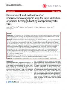
With the availability of real-time data recorded during crashes and near-crashes, it is now possible to evaluate the performance of collision avoidance algorithms using actual events. This report describes a method developed for evaluation of alert algorithm performance using realtime data collected from naturalistic driving. Three alert algorithms are tested using this method. However, the algorithms tested were not production systems. Various measures of driver performance during the events are also presented. The method used in this study was to input naturalistic data collected during actual crashes into models of alert algorithms, and to evaluate the timing of the alert based on kinematics and a distribution of driver reaction time. Real-time data from 13 rear-end (rear-end) crashes and 70 rear-end near-crashes were selected from the 100-Car Naturalistic Driving Study data for analysis. Thirteen crashes from the original dataset were used in the present analysis. These crashes represent all of the cases where video and vehicle data were available of a subject vehicle striking the rear end of a lead vehicle (LV) that was traveling in the same lane. Sixty of the rear-end near-crashes were selected randomly, from approximately 400 rear-end near-crashes recorded in the original data set. An additional 10 near-crashes were included that represented cases where a rear-end crash was avoided through the driver departing the lane to avoid colliding with an LV. Once these events were selected, the data was prepared for further analysis and put into models of collision avoidance algorithms. Three collision avoidance system (CAS) algorithms were selected and modeled for evaluation. 1. Knipling et al. (1993) – Equations developed by Knipling et al. for LV-stationary (LVS) and LV-moving (LVM) scenarios. 2. CAMP Linear – The linear regression approach described in early CAMP work (Kiefer et al., 1999) that predicts a required deceleration after response based on test-track braking by drivers in different scenarios. 3. NHTSA – An algorithm developed by Brunson et al. (2002) that incorporates multiple warning levels and sensitivity settings. When the data from the events were put into the algorithm models, a time-series (i.e., measures tracked over time, rather than at one point in time) output was generated that could be overlaid on the real event data. A kinematic analysis of the real event data was performed to determine the last point in time during the events where three different levels of braking (0.5g, 0.675g, and 0.85g) would be required to avoid collision. The comparison of when the braking needed to begin at a given level to the time when an alert would occur provided a time difference (potentially negative), which was the available time for drivers to respond. This available time was converted into an estimate of the percentage of the population who could respond in the available time for the events tested. xii

This estimate was used as the evaluation of the benefit of the specific alert algorithms. Additionally, an estimate of the frequency with which each of the alerts might occur in normal driving was also developed by inputting files describing entire drives (i.e., trips) into the alert models and counting the number of times the alerts occurred. Various driver behavior and performance measures were also collected during the events. Driver visual behavior measures were collected to support consideration of eye-tracking as a potential parameter in algorithm logic and to explore the relationship between proposed perceptual thresholds and glance behavior. The location and duration of driver glances during the 4.5 s prior to response or collision were captured and related to alert timing and stimuli, such as rate of visual expansion of the LV and whether the LV brake lights were on or off. Driver braking behavior was characterized using the means, the maximums, and the time to reach the three levels of braking used in the kinematic analysis. By using the results of the kinematic analysis, the events themselves were characterized in terms of time available for response and the level of braking needed. The method used in this effort is presented in Figure 1 and provides the methodological organization of this report.

xiii

Original 100-Car Data Collection

Data – Vehicle sensor time-series values

Conversion Data Read

Data Visualization Software

Variable Computation & Reconstruction

Data - Eye glance and LV brake at each change in state

Cumulated Real Event Data

Kinematic Analysis

Driver Performance Measurement

Algorithm Model – Knipling et al.

Algorithm Model – CAMP Linear

Algorithm Model – NHTSA

Time series of alert states

Time series of alert states

Time series of alert states

Alert Data

Cumulated Alert and Real Data

CAS Evaluation Percent able to respond

Frequency of Alerts

Figure 1. Overall Method Schematic ALGORITHM EVALUATION METHOD The algorithm evaluation methodology developed here provides useful guidance both in estimating benefits achieved by the algorithms and in estimating frequencies of alerts in normal driving situations. By computing time available from alert presentation to the need for braking, the method avoids defining the “start” of an event. The method could be improved by accommodating different reaction-time estimates based on whether the driver was already braking at the time he or she detected the event. Estimation of the frequency with which crashes similar to those tested occur across the country, and adjustment of benefit estimates accordingly, may also be informative. The method provides an informative alternative for system developers. It can provide evaluation of systems or system components, it tests systems in a non-hazardous manner, it can be conducted earlier and at lower cost than field operational trials, and permits benchmarking algorithm alternatives. As with any safety-related system, multiple independent approaches are recommended during testing and evaluation.

xiv

ALGORITHM PERFORMANCE When considering the algorithm performance on the 83 events tested, the Knipling and CAMP Linear algorithms had higher percentages of the population who could respond in time to avoid collision (Table 1) compared to the NHTSA algorithm. Table 1. Population who Could Avoid Collision Estimated at Different Deceleration Levels Estimated Percentage of the Population Who Could Avoid Collision

Algorithm

Braking Level Maintained

After Response

Knipling CAMP Linear NHTSA Early NHTSA Intermediate NHTSA Imminent

0.5g mean 47% 56% 30% 26% 25%

0.675g mean 55% 63% 36% 32% 33%

0.85g mean 57% 64% 37% 33% 35%

However, further analysis of the frequency with which the algorithms might generate alerts in normal driving conditions indicates alert frequencies for the Knipling and CAMP Linear alerts as being unacceptable to drivers. The NHTSA alert frequency is closer to what might be acceptable, but would still probably alert too frequently. Table 2 provides a summary of the estimated alert frequencies for the three algorithms. Table 2. Estimated Number of Alerts per 100 Miles Driven Algorithms

Knipling 83

CAMP Linear 87

NHTSA Low Sensitivity 8

This alert frequency analysis was conducted on three trips. As systems are developed and alert frequency counts are reduced, a more structured analysis will be appropriate. The actual average driver braking levels used in the events appear to be closer to 0.5g than to the higher levels evaluated. A 0.5g deceleration in the near-crashes was approximately an 85th percentile mean braking level. Using 0.5g as the expected average braking of a driver, it appears that 20 to 25 percent of drivers would avoid collisions similar to those included in this testing when using the NHTSA algorithm early warning generated while set at a “High” sensitivity. Based on the events identified in the original 100-Car Study data collection, it appears that the collision algorithms do not currently address a common form of rear-end collision. Twenty percent of the events selected from the 100-Car Study data involved a following-vehicle (FV) speed prior to driver response of less than 10 mph. The FV speed prior to driver response was

xv

less than 20 mph in one-quarter of the events. Figure 2 portrays the estimated benefit of the tested algorithms according to the FV speed prior to driver response.

Figure 2. Percentage Avoiding With 0.5g Deceleration by Speed As can be seen, except for the Knipling algorithm, drivers exposed to low-speed collisions will not be warned by the tested algorithms. DRIVING PERFORMANCE In the 4.5 s prior to response in the events including a response, and prior to collision in events without driver response, the driver was looking away from forward for approximately one-third of the elapsed time. In these crash and near-crash events, 17 involved drivers were looking away for driving-related tasks, whereas 14 cases involved looking away from forward for non-driving related tasks. In 44 of 83 events, drivers looked away from the LV although its brake lights were illuminated. These cases include both LVS and LVM events. It also appears that looking away for driving-related reasons is common in situations where the LV is decelerating (or decelerates unexpectedly). It appears that glances away for driving-related reasons may frequently coincide with unexpected LV braking.

xvi

When responding to an event, the mean deceleration achieved by drivers appears to be much lower than the maximum deceleration. The 90th percentile mean deceleration was 0.55g while the 90th percentile maximum was 0.95g. Avoiding the events by braking would have been successful in all cases by starting a 0.5g deceleration as late as 2.0 s prior to the predicted (or actual) point of impact.

xvii

xviii

CHAPTER 1: INTRODUCTION

BACKGROUND

This report explores the use of real crash data to investigate the potential role of specific crash avoidance systems in preventing near-crashes and actual crashes using the driving data collected in the 100-Car Study (Dingus et al., 2006). This data provides unique opportunities for transportation researchers as data was collected in 100 cars for a period of 12 to 13 months per driver. The data represent normal, daily commuter driving with all the stress and pressures that occur in the Northern Virginia/Washington, DC, urban environment. The rear-end crash type and CAS was selected for analysis in this research because: 1. Rear-end CAS systems are currently being tested and released by automotive

manufacturers, and

2. The prevalence of rear-end crashes. The second chapter of this report is a review of literature that relates to rear-end crashes. The review covers factors including time-to-collision estimation, visual sampling, driver performance, and descriptions of rear-end CAS algorithms. The third chapter of the report describes the methods used to prepare the real event data for analysis and the methods used to investigate the potential of rear-end CASs in helping drivers avoid crashes. The fourth chapter presents the results of the analysis. Driver response during the events and timing of potential CAS alerts are characterized according to factors discussed in the literature. The final chapter provides summary and conclusions.

1

CHAPTER 2: LITERATURE

The rear-end crash type encompasses collisions that occur when the front of a following vehicle (FV) strikes the rear of a lead vehicle, with both traveling in the same lane (Martin & Burgett, 2001). This rear-end crash classification can further be separated into more specific crash types: collisions that occur when the lead vehicle is stationary or when the lead vehicle is moving. LVS crashes typically occur when the lead vehicle has stopped and then is struck by another vehicle. LVM crashes usually occur when the LV is decelerating when struck or traveling at some slower speed than the striking vehicle. However, the LV may occasionally be accelerating when hit. Rear-end crashes make up a large portion of crashes occurring on the Nation’s roadways. A 1995 approximation based on accident databases and police reports indicated rear-end crashes account for 25.2 percent of crashes, with 16.1 percent of all crashes being lead-vehicle-stationary and 9.2 percent being lead-vehicle-moving (Najm et al., 1995). However, Dingus et al. (2005) found that in 82 total crashes/collisions recorded during their data collection, only 15 were police-reported. Dingus et al. estimate that crash involvement may be more than five times higher than police-reported crashes. The main objective in implementing rear-end CASs is to reduce the number of rear-end collisions. In order to estimate the potential for rear-end CASs to reduce the number of rear-end collisions, it is helpful to understand both the major causal factors in rear-end collisions and how the CASs are intended to operate to avoid the rear-end collision event. The availability of real crash data also provides the opportunity to relate actual events to a range of human-perceptionrelated and performance-related variables that are found in driving literature, and so will quantify or describe real events according to measures that have been used historically in collisionavoidance research. This research effort will also begin a process of determining which of these measures may provide the most guidance for collision avoidance efforts when using real event data. TIME-TO-COLLISION Drivers constantly make judgments about how to adjust speed based on what is seen in the roadway ahead. If there is a turn ahead, a stop sign, or an obstacle of some kind, drivers are consistently able to account for what is seen and to appropriately adjust the vehicle’s speed throughout. Much of collision avoidance research investigates the ability to judge when braking is necessary to avoid an accident. Additionally, once a driver is braking, the driver must monitor and adjust the level of braking input to brake successfully. Time-to-collision is frequently used in literature as a descriptor of how urgent a situation has become, as well as potentially how a driver perceives stimuli during an event. Time-to-collision can be calculated or approximated using various measures and theories. In an event with a following and a lead vehicle, time-to-collision when approaching a stationary LV, or when the LV is moving at a constant rate (zero acceleration) is computed as, r , [1] TTC  vr

2

where r is the range between the vehicles and vr is the relative velocity, which is defined as

vr  vLV  vFV , [2] where v LV is the velocity of the LV and v FV is the velocity of the following vehicle. Time-to-collision computed in this manner will be referred to in this document as TTC. If the FV acceleration is assumed to be zero and if the LV is accelerating (or decelerating), this LV acceleration is included in the equation as follows:  vr  vr2  2aLV r , [3] TTCa  aLV where aLV is the acceleration of the LV (negative for a deceleration). Time-to-collision where acceleration of the LV (typically deceleration) is included will be referred to as TTCa. Judging TTC (or TTCa), for example in avoiding collision during locomotion, is part of survival in any animal. So, we know that elements of the skill in judging time-to-collision are probably part of our biological make-up. At this point, however, it is not clear exactly what elements of our visual stimuli, as well as stimuli to other senses, are used in the judgment. Components of the judgment include range and closing speed, and these are frequently believed to be evaluated in terms of the visual angle subtended by an LV and rate of change of a visual angle. The visual angle of an LV at any point in time is denoted as  , and is described as,



W , r

[4]

where W is the width of the LV (Hoffmann & Mortimer, 1994). Again, r is the range to the lead vehicle. As the FV closes on the LV, the visual angle will increase at some rate. As an object gets closer,  does not increase linearly. The figure below illustrates how visual angle for a 6-ftwide LV varies over distance (range).

3

Visual Angle (Theta) 6-ft-wide lead vehicle

0.6

35 30 25

0.4

20

0.3

15

0.2

degrees

radians

0.5

10

0.1

5

0

0 0

40

80

120

160

200

240

Range (ft)

Figure 3. Visual Angle Versus Range When drivers are able to perceive a change in  , they are aware that the distance to an LV is changing, but further information is needed to know how quickly the distance is changing. The rate of change of the visual angle during a closing situation is believed to provide this information. The angular velocity (i.e., rate of change of the visual angle) with respect to time is denoted  (thetadot). Using the small angle approximation, the stimulus is described as

 

W (vr ) , r2

[5]

where W is the width of a lead vehicle, r is the range to the lead vehicle, and vr is the difference in velocity between the two vehicles (i.e., relative velocity or V, negative when closing; Hoffmann and Mortimer, 1994). Research relevant to collision avoidance has considered the following:  Time-to-collision-related stimuli such as speed and range (Cavallo & Laurent, 1988; Tresilian, 1991);  Visual angle (Mortimer, 1990; Hoffmann & Mortimer, 1994, 1996; Shiff & Detwiler, 1979; Regan & Hamstra, 1994; Regan & Vincent, 1995);  Rate of change of visual angle (Hoffmann & Mortimer, 1994, 1996; Regan, Hamstra, & Kaushal, 1992); and  The ratio of the previous two values (Regan & Hamstra, 1994; Tresilian, 1991). Measures used by these previous researchers were used in the analysis of the crashes and nearcrashes to quantify the situation at different points in time during the event. Hoffmann and Mortimer (1994, 1996) conclude that the rate of change in the visual angle (i.e.,  ) of an LV, needs to be above approximately 0.003 to 0.004 rad/s for a human to be able to perceive the LV’s relative speed. When the angular velocity was above this threshold, error in

4

estimates was linearly related to the actual TTC and short viewing times were required to estimate TTC. When angular velocity was below threshold, error was not related to TTC. In this case, spacing changes (i.e., visual angle changes) were required to determine TTC, and subsequently the process took longer. Hoffman and Mortimer estimate that between 2 and 20 percent of drivers may overestimate a TTC in conditions similar to those tested (TTC < 10 s and viewing time between 1.37 and 2.74 s). The authors tentatively propose that this may explain some rear-end collision situations and indicate that the angular velocity is the quickest and most accurate method of evaluating TTC, but at longer TTCs, angular velocity may not be above the threshold. Therefore, detection of a change in distance may be required. Detection of this change is proposed to have a just-noticeable difference of 0.12  , or for small angles, 0.12r. Hoffman and Mortimer also indicate that the direct  mechanism, proposed by Regan and Hamstra (1994) may be at work in judging TTC. Regan and Hamstra propose that humans are able to directly perceive TTC, rather than working with the subcomponents of visual angle change and rate of visual angle change. Barton, Cohn, Nguyen, Nguyen, and Toyofuku (2004) and Barton and Cohn (2005) report results of some recent fundamental research that contradicts the  -threshold theory and argue that detection of TTC is actually governed by signal-detection theory. They argue that the threshold theory of Hoffman and Mortimer would indicate 100-percent detection above the threshold, and that the signal-detection theory describes a variable criterion that observers employ based on cost and reward of detecting the signal or missing the signal within the noise of the visual scene. While the findings are based on work that is significantly different from actual driving, it is worth including here for completeness. TTC at Braking Onset Kiefer et al. (1999, 2003) provide measures of driver TTCs at the onset of braking or steering while having drivers brake or steer at the last second according to “normal” and “hard” instructions in several approach scenarios (see discussion in the rear-end CASs section of this paper for more detail). Due to the experimental “normal” and “hard” response instructions in the alerted trials, participants probably were able to perceive the approach earlier, but waited to brake until the last moment. Additionally, as opposed to the other TTC investigations described so far, participants in Kiefer et al. were not reporting when they think the vehicles will hit. The participants indicated when they needed to start their deceleration to avoid the impact. The following values are approximated from graphs in the paper and it is unknown if any statistically significant differences are present. The discussion is intended to provide general reference points. When approaching a stationary vehicle, “hard” onset of braking for a 30-mph approach to the stationary vehicle was 2.5 s TTC. For a 45-mph approach, the TTC at onset was 3.1 s (Kiefer et al., 2003, p. 23). Two scenarios in which the LV was traveling at a slower but constant speed can be compared easily to these because they have relative speeds (vr) which are the same as the described stationary trials. In one, the LV is traveling at 30 mph and the participant is approaching at 60 mph, making a relative speed of 30 mph. The TTC at brake onset for this scenario was 4 s, which is 1.5 s later than in the LV-stationary equivalent. For another condition, the LV was traveling at 15 mph, and the participant was approaching at 60 mph. TTC at brake onset here was also about 4 s, which is about 0.9 s later than for the same relative speed scenario (vr = 45 mph) where the lead vehicle was stationary. So, people braked

5

later for LVS scenarios than for an LV moving at a constant speed, though the difference in speed was the same. If the Kiefer et al. (2003) values are translated into rate of change of visual angle, it appears that in all except the two most extreme of the LV-at-constant-velocity and LVS scenarios, participants were responding where the threshold theory indicates they are able to judge  . In the two most extreme scenarios, where the participant was traveling at 60 mph and either approached a stationary vehicle or an LV traveling at 15 mph, the threshold theory would indicate the braking onset was roughly on the line of where the rate would become detectable. For a 60-mph relative-velocity approach, the threshold estimates  would become detectable at 4.8 s TTC and for a 45-mph relative-velocity the value is 5.5 s. Kiefer et al. (2003) found “hard” braking onset at about 4 s TTC and “normal” braking onset at about 5.2 s TTC. Steering input for these scenarios were about 1 s lower TTC for these same scenarios, occurring at roughly 4 s TTC for the “normal” and 3 s TTC for the “hard.” Based on these comparisons, and according to the threshold of 0.003 rad/s, it appears the participants were able to judge the TTC prior to steering inputs. However, for the extreme scenarios, the participant may need to make the braking decision prior to having sufficient perception information about the scenario. VISUAL SAMPLING Across studies, inattention is identified as a primary causal factor in rear-end crashes (Najm et al., 1995; Knipling et al., 1993; Dingus et al., 2006). Dingus et al., which is the same data on which the present analysis is based, indicate almost 80 percent of the recorded crashes involved the drivers looking away from the forward roadway at the start of the events. In normal driving situations, visually monitoring the roadway is used to maintain lane position and to avoid objects and traffic on the roadway. Additionally, if a driver is not looking forward, it is difficult to see and avoid an unexpected problem. However, drivers look away from the forward path for both driving and non-driving reasons. Understanding what is known about the visual behavior of drivers may provide helpful insight in avoiding collisions.

Knipling et al. (1993) identify a number of causes of inattention in general driving, including several that might arise that do not indicate carelessness by the driver, for example, looking at vehicles beside the road, watching a pedestrian, looking for landmarks, or watching other vehicles. These are issues of attention allocation, each of which could be part of the primary task of driving. As the driver allocates attention, at times the focus will be drawn away from the region where threats may be revealed. There are a number of other sources who describe visual behavior while driving. Measures of visual behavior include glance frequency to different locations in and around the vehicle, duration of glances, and probability of glances (Mourant et al., 1969; Mourant & Rockwell, 1970, 1972; Mourant & Donohue, 1974; Wierwille, 1993). When following an LV, more time appears to be spent monitoring the forward road scene than when not in a following condition. In a car following task, Mourant, Rockwell, and Rackoff, (1969) found that on a familiar route, approximately half the time was spent looking at the lead vehicle and one quarter of the time looking generally ahead. This means 75 percent of the time was looking forward while following and the remaining 25 percent of the time was distributed to out of view glances, road markers, signs, etc. When not following, looking forward made up approximately 60 percent and the remaining 40 percent of the time was used looking elsewhere.

6

Merging and lane changing are examples of driving tasks that require glances away from the forward view. Mourant and Donohue (1974) investigated the use of two different field of view mirror systems during lane changes, merges, and while driving straight ahead. The mean number of glances away from the forward roadway during the lane change and merge maneuvers, either in a head turn or when looking at mirrors, was between approximately 2.5 and 3.5. Total mean time looking away from the forward roadway during the maneuvers was between approximately 2 and 3.25 s. Head turns involved more time away from forward than mirror use. Tijerina (1999) provides an alternative look at visual behavior by investigating the conditions in which drivers shift visual attention away from the forward scene. He measured the frequency of glances away during a car-following epoch, duration of the glances away, and location of the glance (gaze location). He found that drivers look away when range rate is approximately zero, regardless of range. He then went on to explore the theory that drivers use optical expansion to decide when it is safe to look away. He found that with a closing gap, 81 percent of the conditions where a driver looked away were below the 0.003 rad/s threshold. The 19 percent of the glances taken away from the forward view occurred when the range rate would have been detectable according to the threshold, and are believed to include overtaking- and passing-related glances. A second finding was that as the duration of the car-following epoch increased, the number of glances away increased, per following epoch. A linear regression relating glance frequency to glance duration was developed as

f GA  1.84  0.17t f ,

[6]

where fGA is the frequency of glances away and tf is the duration of the following epoch. In looking at glance durations, he found a mean glance away duration of 0.6 s with a 5th percentile value of 0.17 s and a 95th percentile of 1.47 s. Tijerina theorizes that these are shorter than found for other researchers because they were glances during following, where other researchers typically report glances across both following and non-following situations. The same regression procedure was used to see if the length of a glance was influenced by range, range rate, or speed. No significant results were found, indicating that glance-away duration may not be guided by our speed, range, or range rate. Tijerina concluded that (1) drivers glance away when range rate appears near zero, without regard to range or speed; and (2) frequency of away glances increases as the length of a following epoch increases. His results support the notion that the static visual scene present in following and the very low frequency of events probably creates a learned behavior of following closer than is advisable for emergency stopping (Evans, 1991). PERFORMANCE When exposed to a stationary object or vehicle, a lead vehicle that has come to a stop, or a rapidly decelerating lead vehicle, the driver will be required to respond. The following discussion reviews efforts to describe the driver’s performance in these situations, particularly in unexpected situations.

7

Human Braking For the purpose of evaluating stopping sight distances for roadway design, Olson and Sivak (1986) measured the time required to perceive a yellow foam rubber block (15 cm high by 91 cm wide) and time to respond to the object by braking. Time from when the object was first visible to when the participant released the accelerator (called perception time in Olson and Sivak’s work), and time from accelerator release to brake press (response time) were measured. These two together are called perception response time (PRT). The speed of 12 to 14 m/s (43.2 to 50.4 km/h or 27 to 31 mph) and average distance when the object was seen of 46 m (151 ft) generated TTCs of 3 to 4 s. The study also measured alerted trials and trials where the participant responded to an auxiliary brake lamp mounted on the hood of the participant vehicle. The 95th percentile PRT was 1.6 s for the surprise scenario. Older participants were found to have slightly longer perception times, but shorter response times in the surprise scenario, making the PRT for old and young essentially the same. Surprise events had reaction times that were longer than those found in situations where the participant was alerted.

Malaterre et al. (1988) provide discussion of a number of approaches to understanding braking and steering responses in emergency situations, including one approach using kinematic reconstructions of accidents. In their summary, they indicate that people tend to use simple responses in emergencies, and braking is the primary response. Two of the authors performed a simulator study (Lechner & Malaterre, 1991) in which 49 participants were exposed to an incurring vehicle at an intersection. The instructed speed was 90 to 100 km/h (56 to 62 mph). The incurring vehicle followed a trajectory to represent indecision, finally stopping in the intersection. TTCs tested were 2.0, 2.4, and 2.8 s, so the ranges were between 35 to 85 m. The first response for 33 participants was release of the accelerator pedal and for 14 was to swerve. The average time to make these inputs was 0.80 and 0.82 s, respectively (not statistically different at =0.05). Average time to get to the brake was 1 s, which is longer than steering (p=0.02). When considering the three TTCs tested, the authors indicate that participants release the accelerator as a reflex, but then the time to brake varies as they process the information. In all, 88 percent of the participants braked. Sixty-seven percent began by braking but steered as well. In 39 percent, only braking was used. The authors conclude drivers prefer to brake only, if they have time. Lechner and Malaterre also explored crash and no-crash outcomes by reducing reaction times on the crash incidents, but maintaining inputs and trajectories. They find that if a reduction in reaction time of 25 percent could be achieved, it would help several of the steering responses be successful. However, even reaction times near zero would not help those who only braked avoid the incident. Lerner (1993) performed a study looking at PRT for 116 drivers of different age groups by releasing a barrel into the road as participants drove their own vehicles on actual roads. The participant’s speed was approximately 40 mph and the barrel was released at a time-to-collision of about 3.4 s (200 ft). Eighty-seven percent of the drivers made some maneuver, with 43 percent steering and braking, 36 percent only steering, and 8 percent only braking. From this, 51 percent used braking in their response. For 56 participants whose brake reaction time could be measured, the mean PRT was 1.5 s (SD 0.4 s). The 85th percentile PRT across all participants was 1.9 s. The two longest values were 2.39 s and 2.54 s. Lerner discusses a lack of differences

8

between older and younger participant PRTs, as well as the impression that older participants moved to the brake more quickly, but younger participants may be using their faster information processing and other capabilities to evaluate and modulate their response. This tends to agree with the age findings of Olson and Sivak (1986) in which participants encountered a foam block. The TTCs when the object became visible in both studies were also similar. Measurements of brake response times for 100 drivers were collected in a simulator study by Broen and Chiang (1996). Male and female participants 18 and older drove a vehicle buck-based simulator with longitudinal acceleration motion cues. As part of a larger test looking at pedal configurations, participants drove a trial where an unexpected obstacle was presented. Among other traffic rules and lane maintenance instructions, participants were told, “an unexpected obstacle may appear in the vehicle’s path and in that event they should step on the brake and stop as quickly as possible” (Broen & Chang, 1996, p. 901). In this work, reaction time starts when the obstacle (a pedestrian) steps into the lane and stops when foot movement begins. Response time is defined as reaction time plus movement time. Accelerator and brake pedal actuation is flagged in the video using lights mounted under the instrument panel and within the view of the camera. Start of foot movement was marked by release of the accelerator pedal. Movement time ended at activation of the brake pedal. Sample rates are not discussed. However, a video camera was used to collect movement time, potentially indicating sample rates of 30 Hz. The work did not find a significant effect (=0.05) on brake pedal response time or movement time for the three lateral pedal layouts tested. The older age group (51 and older) had slower response times than the two younger groups (18 to 30 and 31 to 50 years old). Based on instructions, participants were going 25 mph at the time the obstacle was introduced. The mean time to reach the brake pedal from entry of the obstacle was 1.33 s. Because perception-response times are skewed right, it is helpful to review Figure 4, which presents the percentiles of responses for the three different pedal layouts. The differences across age groups for this study are shown in Table 3.

Figure 4. Brake Pedal Response Time (Broen and Chang, 1996, p. 903)

9

Table 3. Braking Response Times (Broen and Chang, 1996, p. 904)

In a test-track study, driver response to a vehicle incurring at an intersection was measured (Mazzae, Barickman, Forkenbrock, & Baldwin, 2003). In this study, after repeatedly passing an intersection with real crossing traffic present, the participant approached a full-size photograph of a vehicle (the photograph had been pulled into the intersection). Mean time to initial brake press here was 1.5 s (SD 0.30 s). This is compared to a similar driving simulator study (Mazzae, Baldwin, & McGehee, 1999), which is described in the steering response section of this report. Maximum deceleration in the test-track study was 0.65g and in the simulator was 0.8g. It appears these values are means across the participants. A simulator study was conducted investigating braking with and without ABS during an intersection incursion scenario similar to those discussed previously (McGehee, Mazzae, Baldwin, Grant et al., 2000). An incurring vehicle enters from the right at a time-to-intersection (TTI) of 2.5 s or 3.0 s. A mean time to accelerator release of 0.94 s was found, with a time to brake application of 1.1 s, for a 3.0 s timeto-intersection event. In a simulator study looking at an incurring pedestrian, Barrett, Kobayashi, and Fox (1968) used a pedestrian entering the participant’s path at approximately 2.25 s TTC. Brake reaction time in this study appeared to range from approximately 0.8 s to 1.4 s for the 11 participants. In a much later simulator study, Araki and Matsuura (1990) exposed 32 novice and experienced drivers to an unexpected pedestrian running into the road from the right at approximately 1.8 s TTC. Braking was the most common response, with 78 percent of participants braking. Of people who did steer, 78 percent also braked.

10

Figure 5 provides a summary of the time-to-accelerator-release and time-to-brake-press values for seven of the studies reviewed here.

Figure 5. Mean Response Times Comparison Across Studies

These measures are a mix of means and 50th percentiles, some of which were approximated from report graphs and should not be considered too precisely. It appears accelerator-release means range from 0.7 to 1.3 s and brake press from 1 to 1.5 s. Distributions would be skewed towards higher values. REAR-END CASS The term CAS here is used to describe any system that either warns the driver to assist them in avoiding a collision, or potentially intervenes in vehicle control in some way that helps to avoid a collision or reduce the effects of a collision. Levels of CASs can be defined according to the level of intervention during an event. Najm et al. (1995) provide a representation of time from initial threat to collision, and the different levels of CASs that might be employed. Figure 6 presents the different levels of CAS as time diminishes before a crash.

11

Figure 6. Intensity of CAS Action (from Najm et al., 1995)

The progression of events portrayed in Figure 6 is as follows. As an initial threat develops during normal driving, the first course of action for a CAS might be to provide a warning of some kind, such as a visual indicator or auditory tone. As time progresses, and options are reduced, an intervention of some type may be appropriate, such as push back on an accelerator. In the last instant, it may be appropriate for a CAS to take full control of a vehicle to decelerate it. This may be determined by the point where the driver is no longer capable of providing a response in time to avoid either due to human performance limitations, lack of detection and recognition, or incapacity. Finally, the crash becomes unavoidable. Driver warning systems include, for example, a forward collision warning (FCW) system that alerts the driver to an obstacle without exerting any control over the vehicle. A headway display is another type of warning system that might communicate to the driver when the following behavior is considered dangerous. Adaptive cruise control (ACC) is a type of cruise control that is capable of deceleration according to presence or deceleration of a lead vehicle. The haptic feedback provided by the deceleration as well as the reduction in speed means the system bridges the definition between a warning and a control system. The haptic feedback can be considered a form of graded warning system as well, in that more severe situations will provide more severe deceleration. These systems do not necessarily warn for a stationary target, however, and are currently limited to approximately 0.25g, approximately 25 percent of a typical vehicle’s braking capability. A system which is capable of full automatic control of braking or steering would probably operate in the shortest time separation before a potential collision. Although in some literature CAS refers to only this final level, this report considers the human as part of the overall system, and so warnings to the driver are included in CAS consideration.

12

An important component of assessing the role of CAS is to understand the underlying algorithms that will be employed in the systems. The CAS algorithm is a formula that uses sensor data as inputs and attempts to determine when a collision warning or intervention should occur. The following sections describe three algorithms that have been proposed for making these alert decisions. Knipling et al. (1993) The early algorithm work of Knipling et al. (1993) describes two straightforward equations that are presented as a possible prototype headway-warning algorithm. Knipling et al. developed a set of equations to identify a warning range (rw) required for stopping given an LVS or an LVM situation. Using FV speed (vFV), time delay of the driver and braking system (td), and deceleration level of the host vehicle (aFV), the equation will predict the range at which a warning should occur. The equation for warning range in an LVS (Knipling et al., 1993) situation is,

rW  t d vFV

2 v FV  . 2a FV

[7]

For an LVM (decelerating) condition, the equation becomes rw 

2 vFV v2  t d v FV  LV , 2a FV 2a LV

[8]

where acceleration of the LV (aLV) and speed of the LV (vLV) make up the additional term (Knipling et al., 1993). The estimated time delay of the driver and braking system combined developed by Knipling et al. was 2.05 s. A method of using driver reaction time alternatives was discussed. Using a reaction time two standard deviations above the mean and two standard deviations below the mean would permit analysis of different outcomes. The model obviously does not vary factors such as the level of FV deceleration, timing of response according to display modalities, or the influence of other factors such as driver adaptation, false alarm rates, or following conditions. CAMP Linear Algorithm (Kiefer et al., 1999 & 2003) The Collision Avoidance Metrics Partnership looked at LVS and LV-braking scenarios (Kiefer, LeBlanc, Palmer, Salinger, Deering, and Shulman, 1999). One hundred eight drivers performed “normal” or “hard” last-second braking or steering maneuvers while approaching an LV traveling at a constant speed or decelerating according to some controlled profile. For “normal” braking, participants were instructed “to maintain their speed and brake at the last second possible to avoid colliding with the target using ‘normal’ braking intensity or pressure” (Kiefer et al., 2003, p. 11). For “hard” braking, participants were instructed “to maintain their speed and brake at the last second possible to avoid colliding with the target using ‘hard’ braking intensity” (Kiefer et al., 2003, p. 11). “Normal steering” instructions were, “to maintain their speed and change lanes at the last second they ‘normally would to go around the target’ ” (Kiefer et al., 2003, p. 12). The “hard steering” instructions were “to maintain their speed and change lanes at the last second they ‘possibly could to avoid colliding with the target’ ” (Kiefer et al., 2003, p. 12).

13

The approach is intended to isolate kinematic conditions (i.e., FV speed, LV speed, and LV deceleration) that necessitate what would be considered “hard” last-second braking, from all of the conditions that would be considered “normal” last-second braking for an alerted driver. When the situation ahead necessitates a hard-braking response (according to what was collected), the alert should be appropriate. The CAMP method used a lead vehicle towing a full-sized mock-up of the back of a vehicle (known as a surrogate target) on a 40-ft telescoping boom. One outcome of this was the Required Deceleration Model that uses the required deceleration necessary to estimate alert timing. Another outcome from this work was an estimate of driver brake reaction time, which was developed based on unexpected scenarios. The required deceleration at the time of participant response as well as various TTC- and TTCa-related measures were used in reporting results. Kiefer et al. (2003) sought to identify the human braking and steering behavior in additional scenarios, or kinematic conditions, from the previous work. To the two previous scenarios ( LVstationary and LV-braking), a scenario with LV traveling at a slower but constant speed was added. Seventy-two drivers in three age groups (20 to 30, 40 to 50, and 60 to 70 years old) participated. The three types of scenarios were as follows: 1. LV-stationary – The participant approached a stationary vehicle at either 30 or 60 mph. The participant waited until the last second to brake or steer, depending on the instructions described previously. 2. LV-braking – with either a stable “normal” headway for the driver, or 3 s headway, and at either 30 or 60 mph, the LV would decelerate at 0.15g or 0.39g with brake lights. The participant waited until the last second to brake or steer, depending on the instructions. 3. Constant relative speed – Speed combinations between the participant vehicle and LV were 30 mph/20 mph, 30 mph/10 mph, 60 mph/50 mph, 60 mph/30 mph, and 60 mph/15 mph, generating relative speeds (vr) of 10 mph, 20 mph, 10 mph, 30 mph, and 45 mph respectively. The participant waited until the last second to brake or steer, depending on the instructions. The participant steering responses in the 60-mph trials tended to occur later than braking responses, whereas in the 30-mph trials, timing differences between steering versus braking were not observed. A greater difference in speed (vr) between the approaching participant and the LV resulted in a greater difference in braking onset time versus steering onset time. From a database of approximately 3,500 last-second braking trials and 800 last-second steering trials, two braking onset algorithms were developed. One algorithm uses a linear regression analysis to describe decelerations the drivers employed and one used logistic regression. The inputs used to develop the linear regression analysis are relative speed (vr), LV acceleration (aLV), and whether the LV is moving or stationary. The results of this analysis are nearly identical to the Required Deceleration Model developed in their earlier work (Kiefer et al., 1999). The warning algorithm inputs the vehicle’s current speeds and accelerations into the

14

linear regression model to evaluate the need to warn. The progression of computations the model uses to predict the warning time is summarized in Figure 7. Vehicle and Radar data: vFV, vLV, aLV, aFV

Total Delay Time = Driver RT + brake system delay

Estimated Vehicle States After Delay vFVP = f(vFV, aFV, td) vLVP = f(vLV, aLV, td)

Case 1: Start: LV stationary End: LV still stationary

Deceleration Required drqd=f(aLV, vLV, vFV)

Delay Time Range rd =f(vFV, vLV, aFV, aLV, td)

Brake Onset Range 1: BOR1=f(Est vFVP, drqd)

Case 2: Start: LV moving End: LV still moving

Brake Onset Range 2: BOR2=f(vFVP, vLVP, drqd, aLV)

Case 3: Start: LV moving End: LV has stopped

Brake Onset Range 3: BOR3=f(vFVP, vLVP, drqd, aLV)

Warning Range rw= BORn + rd

Figure 7. CAMP Warning Time Prediction Logic

Equations or initial values for each of the functions in the flowchart are as follows: The prediction of the velocity of the FV after the delay (vFVP) is vFVP  vFV  (aFV )td ,

[9]

where aFV is the acceleration of the FV and td is the time delay before driver and vehicle response begins. Similarly, the predicted velocity of the LV (vLVP) is vLVP  vLV  (aLV )td .

[10]

The deceleration required for the FV, based on the linear regression analysis of driver responses is

d rqd  5.308  0.685a LV  2.570(v LV  0)  0.086(v FVP  v LVP ) ,

[11]

where values are in ft/s and ft/s2. The range lost during the response delay (rd) is defined as rd  (vFV  vLV )td  0.5(aFV  aLV )td2 .

[12]

15

Three cases are used to account for the state of the LV before and after the response delay and to select from the appropriate equations. Case 1, in which the LV is stationary throughout, uses the brake onset range (BOR1) equation BOR1 

2 vFVP .  2d rqd

[13]

Case 2, in which the LV is moving initially and still expected to be moving after the delay, uses the brake onset range (BOR2) equation BOR2 

(vFVP  vLVP ) 2 .  2(d rqd  d LV )

[14]

Case 3, in which the LV is moving initially but expected to stop by the time response begins, uses the brake onset range (BOR3) equation

BOR3 

2 vFVP v2  LVP .  2d rqd  2d LV

[15]

The logistic regression model, which proved to be as accurate as the linear models, but with lower required input accuracy, evaluates the probability that the driver is in a last-second hard braking situation rather than a last-second normal braking situation. The inputs to the model are relative speed (vr), range (r), which are used to compute an inverse TTC value: vr 1  . r TTC

[16]

Then, a rough categorization of LV deceleration (aLV) is used to choose from three categories. The three categories are LV stationary, LV moving and braking, and LV moving and not braking. A separate equation was developed for each of these three scenarios. For these reasons, this model is referred to as the “3-Tiered Inverse Time-to-Collision Model.” It models the driver’s braking response as being based on an inverse TTC threshold that lowers linearly with speed—the driver becomes more sensitive as speed increases. In more detail, in the logistic regression method, the kinematic conditions (vFV, vLV, and r at braking) of a number of last-second braking trials, together with their associated “hard” or “normal” instruction, can be converted into a function. The conditions associated with “hard” instructions are assigned a 1, indicating these are warning events. The conditions associated with “normal” instructions are assigned 0, because the warning should not occur for these. A formula is then developed to translate the inputs (kinematic conditions) into some value x. For example, x=f(vLV, vFV, r). A probability model is developed using x, in this case p=1/(1+e-x). In a driving situation, the kinematic conditions are fed into the probability equation, to give some probability that what the sensors see is a “hard” braking event. If the probability of this observed situation exceeds a probability threshold, then a warning should be presented. The probability threshold is

16

either selected by warning system designers, or potentially could be based on some driver characterization over time. The flow chart in Figure 8 describes the progression from developing the logistic regression equation based on the “hard” and “normal” last-second trials, to testing real-time conditions using the regression equation, and finally comparing it to a probability threshold to decide whether to alert or not. Logistic Regression Last second trials Vehicle and Radar data: vFV, vLV, r

Instructions “hard” or “normal”

p(hard given vFV, vLV,r)

Real-time Test

x=ln((1/p)-1

Current vFV, vLV, r

Develop equation for x x=f(conditions)

x=f(vFV, vLV, r)

Designer p(threshold) p=0.75

Curent p(hard given current conditions)

If current p greater than Designer p, then alert.

Figure 8. CAMP Logistic Regression Logic Diagram

The 3-Tiered Inverse TTC approach identified separate equations for the three different LV states; (1) lead vehicle moving and braking; (2) lead vehicle moving but not braking; and (3) lead vehicle stationary. Three coefficients (a, b, and c) from the appropriate equation are input into a brake onset range equation, b(v FV  v LV ) , [17] 1 ln( 1)  a  c(v FV ) p where p is a probability value. A value of 0.75 is considered a promising p value by Kiefer et al. The equations are predicted to generate an alert in about 15 percent of the cases where a driver was aware, and intending to steer later, rather than brake. This is because the three equations are BOR 

17

developed based on when the driver would brake at the last second, and because this braking would occur earlier than last-second steering. NHTSA Algorithm (Brunson et al., 2002) NHTSA worked with the Johns Hopkins University Applied Physics Laboratory to develop a NHTSA FCW algorithm (Brunson, Kyle, Phamdo, & Preziotti, 2002). The algorithm is only intended to function at 25 mph or above. Separate modes are defined for cases where ACC is active and a tailgating mode is used when the FV is following closely. The algorithm uses a driver-plus-system delay time of 1.6 s if the driver is not currently braking and 0.5 s if the driver is braking. Two somewhat unique aspects of this algorithm description are the inclusion of a driver sensitivity adjustment and also a three-stage (three-level) warning. The NHTSA algorithm uses a lookup table to adjust the maximum expected host vehicle braking (aFVmax) when estimating the collision threat. Driver sensitivity settings include near, middle, and far, which tend to describe how a driver might follow, with far being the most conservative style. The three alert levels are early, intermediate, and imminent. Table 4 provides host vehicle braking levels expected for each of these alert levels. As can be seen in the table, the maximum braking level used in the algorithm is 0.55g. Table 4. NHTSA Alert Sensitivity Settings and Alert Levels

Warning Sensitivity Early 0.38 0.32 0.27

Near Middle Far

Alert Level (aFVmax threshold in g’s) Intermediate Imminent 0.45 0.55 0.40 0.55 0.35 0.55

The first step of the algorithm is to estimate the time it will take both vehicles to come to a stop. Based on the driver’s selected warning sensitivity, during each iteration, the algorithm computes stop times for the FV (tFVs) for each of the warning three levels (differentiated by aFVmax) in parallel, and alerts according to the highest level appropriate. A stop time is also computed for the lead vehicle (tLVs). This calculation describes the time it takes to dissipate speed. Time for the LV to stop is computed as  vLV t LVs  , [18] aLV where vLV is the initial speed of the lead vehicle and aLV is the initial deceleration of the lead vehicle. Time for the FV to stop is computed as

t FVs  tr 

(vFV  aFV tr ) , aFV max

[19]

unless the FV stops before the response time is reached (indicated by a negative value in the numerator of the second term), in which case, TFVs 

 vFV . aFV

[20]

18

Using these estimates of time to stop, a distance required to miss the collision (Dmiss) is computed. In situations where an LV is initially moving, and based on the time computations, is expected to come to a stop before the FV, the following equation is used to calculate the warning distance required to miss the lead vehicle: D miss  r 

1 1 1 (a FV  a FV max )(t r ) 2  a LV (t LVs ) 2  (a FV  a FV max )t r t FVs  v r t FVs  a LV t FVs t LVs  a FV max (t FVs ) 2 . 2 2 2

[21] In situations where the FV is expected to come to a stop before the lead vehicle based on the time-to-stop calculations, or where the LV is initially stopped, a time-to-miss value (tm) is calculated, tm 

vr  (aLV  aFV )tr  tr . aFV max  aLV

[22]

In these situations, Equation 23 is used to estimate the distance needed to warn to achieve a miss. 1 1 Dmiss  r  vr t m  (a LV  a FV max )(t m ) 2  (a FV  a FV max )t m t r  (a FV  a FV max )(t r ) 2 2 2 [23] The three Dmiss values (one for each alert level) are compared to a threshold distance computed as

Dthresh  2  vFV (0.1) ,

[24]

where vFV is in m/s and Dmiss is in meters.

19

CHAPTER 3: METHODS

This project explores the use of real crash and near-crash data for evaluation of CAS algorithms. A process was developed and applied to a set of publicly available algorithms using data collected during actual events. It should be noted that the algorithms tested were not production systems. Figure 9 illustrates the subtasks involved in the methodology. Original 100-Car Data Collection

Data – Vehicle sensor time-series values

Conversion Data Read

Data Visualization Software

Variable Computation & Reconstruction

Data - Eye glance and LV brake at each change in state

Cumulated Real Event Data

Kinematic Analysis

Driver Performance Measurement

Algorithm Model – Knipling et al.

Algorithm Model – CAMP Linear

Algorithm Model – NHTSA

Time series of alert states

Time series of alert states

Time series of alert states

Alert Data

Cumulated Alert and Real Data

CAS Evaluation Percent able to respond

Frequency of Alerts

Figure 9. Overall Method Schematic

Each dashed outline in the figure surrounds a main component or components of the method. The method components include: 1. Original 100-Car Study data collection; 2. Data preparation; 3. Algorithm modeling; 4. Kinematic analysis; and 5. CAS algorithm evaluation. 20

The 100-Car Study data provided the real data in a time-series format. The next component of the method was to take the original 100-Car Study data and prepare it for further analysis and for use by alert algorithm models. Models of the three alert algorithms were developed to read in the real data and output when alerts would occur. This data were then merged with the real data. Also using the real data as a starting point, kinematic analysis was used to quantify the necessary timing and level of braking in each event. Kinematic estimates and alert timing from real data are evaluated against distributions of driver reaction time to quantify whether or not sufficient reaction time was available based on the alert timing and kinematics. The final step in the method was the evaluation of the alerts according to the necessary timing based on kinematics and the frequency in which alerts occur in driving data. Driver performance measurements were also collected using the real-time data for use in further analysis and CAS development. Having described the general method, it is appropriate to consider some of the limitations or assumptions inherent in the method. The approach described uses time-series data collected from instrumented vehicles during actual crashes or near-crashes. Instrumentation used during the collection of data may be different than sensors proposed for a deployable CAS. For example, forward range and range rate sensors may report or not report targets differently, depending on their design. Crashes and near-crashes used in this manner provide examples of events. The events used in this approach first must be located within collected data, and then are reviewed by video reductionists. The target scenario for a CAS may not completely align with the event search procedures or with the classification of events made during video reduction. Within the method, these events are generalized, and records of events of these types are accumulating, but the range of events occurring on the roadways may differ from those located in this type of data. Finally, in this approach, an alert is not actually presented to the driver. Different outcomes could occur upon presentation of an alert. Driver behavior may change immediately or over time in the presence of a CAS. As with any safety-related system, multiple independent approaches are recommended during testing and evaluation. The method described here provides an informative alternative for system developers. This method can provide evaluation of systems or system components, it tests systems in a non-hazardous manner, it can be conducted earlier and at lower cost than field operational trials, and it permits benchmarking algorithm alternatives. The following sections provide additional detail on each of the components outlined with dashed lines in Figure 9. ORIGINAL 100-CAR STUDY DATA COLLECTION For the investigation conducted here, the primary data source is the driving performance data obtained in a subset (13 rear-end crashes and 70 near rear-end crashes) of the crashes and nearcrashes collected in the 100-Car Study. From the original 100-Car Study analysis, these events are defined as follows:

 

Crash: Any contact between the subject vehicle and another vehicle, fixed object, pedestrian cyclist, animal, etc. Near-Crash: Defined as a conflict situation requiring a rapid, severe evasive maneuver to avoid a crash.

21

The crashes included in this subset were selected from the set of FV striking rear-end crashes recorded in the 100-Car Study that had video data available. Sixty near-crashes were selected randomly from among the approximately 400 rear-end near-crashes identified in the 100-Car Study data set. The complete set of 400 rear-end near-crashes were not used to control the scope of the project. Ten near-crashes were also included which were classified as run-off-road crashes in the 100-Car Study. Table 5 describes the ages and estimated annual mileage of the drivers included in the dataset used for this investigation. Sixty-seven different drivers were involved in the investigated events. Drivers in 34 of the events were female, and in 49 of the events the drivers were male. Eleven drivers had more than one event, with 5 drivers having three events and 6 having two events. The remaining 56 drivers had one event each. Table 5. Biographic data for drivers in selected events.

Demographic data for drivers in selected crashes and nearcrashes Average Maximum Minimum

Age (yrs) 35 68 18

Estimated Annual Miles 21,516 75,000 10,000

Two methods were used to provide a review of the potential for algorithms to provide benefit in preventing near-crashes and crashes. The first method was to estimate what type of improvement in driver response time might be expected from a collision warning, and to determine if this would be sufficient for avoiding a crash. This estimate involved review of the crash data, kinematic analysis of time available to respond, and estimates of the percentage of people able to respond and avoid. The second method was to develop a basic measure to consider false-alarm rates of the potential algorithms. For a complete description of the 100-Car Study method, instrumentation, and data collection procedure, refer to the Dingus, Klauer, and Neale, et al. (2006) report. In order to provide an abbreviated description, the following description is provided from Neale, Klauer, Dingus, Sudweeks, and Goodman (2005). 100-Car Study Instrumentation The 100-Car Study instrumentation package was engineered by VTTI to be rugged, durable, expandable, and unobtrusive. It constituted the seventh generation of hardware and software, developed over a 15-year period that has been deployed for a variety of purposes. The system consisted of a Pentium-based computer that received and stored data from a network of sensors distributed around the vehicle. Data storage was achieved via the system’s hard drive, which was large enough to store data for several weeks of driving before requiring data downloading.

Each of the sensing subsystems in the car was independent, so that any failures that occurred were constrained to a single sensor type. Sensors included a vehicle network box that interacted with the vehicle network, an accelerometer box that obtained longitudinal and lateral kinematic information, a headway detection system to provide information on leading or following vehicles, side obstacle detection to detect lateral conflicts, an incident box to allow drivers to flag incidents for the research team, a video-based lane tracking system to measure lane-keeping 22

behavior, and video to validate any sensor-based findings. The video subsystem was particularly important as it provided a continuous window into the happenings in and around the vehicle. This subsystem included five camera views monitoring the driver’s face and driver side of the vehicle, the forward view, the rear view, the passenger side of the vehicle, and an over-theshoulder view for the driver’s hands and surrounding areas. An important feature of the video system is that it was digital, with software-controllable video compression capability. This allowed synchronization, simultaneous display, and efficient archiving and retrieval of 100-Car Study data. A frame of compressed 100-Car Study video data is shown in Figure 10. The driver’s face (upper left quadrant) is distorted to protect the driver’s identity. The lower right quadrant is split with the left-side (top) and the rear (bottom) views.

Figure 10. A Compressed Video Image From the 100-Car Study Data

The modular aspect of the data collection system allowed for integration of instrumentation that was not essential for data collection, but which provided the research team with additional and important information. These subsystems included automatic collision notification that informed the research team of the possibility of a collision; cellular communications that were used by the research team to communicate with vehicles on the road to determine system status and position; system initialization equipment that automatically controlled system status; and a GPS positioning subsystem that collected information on vehicle position. The GPS positioning subsystem and cellular communications were often used in concert to allow for vehicle localization and tracking. The system included several major components and subsystems that were installed on each vehicle. These included the main Data Acquisition System unit that was mounted under the package shelf for the sedans (Figure 11) and behind the rear seat in the SUVs.

23

Doppler radar antennas were mounted behind special plastic license plates on the front and rear of the vehicle (Figure 12). The location behind the plates allowed the vehicle instrumentation to remain inconspicuous to other drivers.

Figure 11. The Main DAS Unit Mounted Under the “Package Shelf” of the Trunk

Figure 12. Doppler Radar Antenna Mounted on the Front of a Vehicle

24

The final major components in the 100-Car Study hardware installation were mounted above and in front of the center rear-view mirror. These components included an “incident” box which housed a momentary pushbutton that the subject could press whenever an unusual event happened in the driving environment. Also contained in the housing was an unobtrusive miniature camera that provided the driver face view. The camera was invisible to the driver since it was mounted behind a “smoked” plexiglas cover. Mounted behind the center mirror were the forward-view camera and the glare sensor (Figure 13). This location was selected to be as unobtrusive as possible and did not occlude any of the driver’s normal field of view.

Figure 13. The Incident Push Button and Camera Box Mounted Above the Rearview

Mirror

100-Car Study Subjects One hundred drivers who commuted into or out of the Northern Virginia/Washington, DC, metropolitan area were initially recruited as primary drivers to have their vehicles instrumented or receive a leased vehicle for this study. Drivers were recruited by placing flyers on vehicles as well as by placing newspaper announcements in the classified section. Drivers who had their private vehicles instrumented (78) received $125 per month and a bonus at the end of the study for completing necessary paperwork. Drivers who received a leased vehicle (22) received free use of the vehicle, including standard maintenance, and the same bonus at the end of the study for completing necessary paperwork. Drivers of leased vehicles were insured under the Commonwealth of Virginia policy.

As some drivers had to be replaced for various reasons (for example, a move from the study area or repeated crashes in leased vehicles), 109 primary drivers were included in the study. Since 25

other family members and friends would occasionally drive the instrumented vehicles, data was collected on 132 additional drivers. A goal of the original 100-Car Study was to maximize the potential to record crash and nearcrash events through the selection of subjects with higher than average crash or near-crash risk exposure. Exposure was manipulated through the selection of a larger sample of drivers below the age of 25, and by the selection of a sample that drove more than the average number of miles. The age by gender distribution of the primary drivers is shown in Table 6. The distribution of miles driven by the subjects during the study appears as Table 7. As presented, the data are somewhat biased compared to the national averages in each case, based on TransStats (2001). Nevertheless, the distribution was generally representative of national averages when viewed across the distribution of mileages within the TransStats data. One demographic issue with the 100-Car Study data sample that needs to be understood is that the data was collected in only one area (i.e., Northern Virginia/Metro Washington, DC). This area represents primarily urban and suburban driving conditions, often in moderate to heavy traffic. Thus, rural driving, as well as differing demographics within the United States, are not well represented. Table 6. Driver Age and Gender Distributions for Original 100-Car Study Dataset

Gender Age N Grand % of total Female Male Total 18-20 9 7 16 8.3% 6.4% 14.7% 21-24 11 10 21 10.1% 9.2% 19.3% 25-34 7 12 19 6.4% 11.0% 17.4% 35-44 4 16 20 3.7% 14.7% 18.4% 45-54 7 13 20 6.4% 11.9% 18.3% 55+ 5 8 13 4.6% 7.3% 11.9% 43 66 109 Total N Total Percentage 39.4% 60.6% 100.0%

26

Table 7. Actual Miles Driven During the Original 100-Car Study Actual Miles Driven 0-9,000 9,001-12,000 12,001-15,000 15,001-18,000 18,001-21,000 > 21,000

Number of Percentage Drivers of Drivers 29 26.6% 22 20.2% 26 23.9% 11 10.1% 8 7.3% 13 11.9%

A goal of the recruitment process was to attempt to avoid extreme drivers in either direction (i.e., very safe or very unsafe). Self reported historical data indicate that a reasonably diverse distribution of drivers was obtained. Vehicles Since 100 vehicles had to be instrumented with a number of sensors and data collection hardware, and since the complexity of the hardware required a number of custom mounting brackets to be manufactured, the number of vehicle types had to be limited for this study. Six different vehicle models were selected based upon their prevalence in the Northern Virginia area. These included five sedan models (Chevrolet Malibu and Cavalier, Toyota Camry and Corolla, and Ford Taurus) and one SUV model (Ford Explorer). The model years were limited to those with common body types and accessible vehicle networks (generally 1995 to 2003). The distribution of these vehicle types was:

     

Toyota Camry – 17 percent; Toyota Corolla – 18 percent; Chevy Cavalier – 17 percent; Chevy Malibu – 21 percent; Ford Taurus – 12 percent; and Ford Explorer – 15 percent.

DATA PREPARATION Modeling the CAS algorithms using real data involves inputting variables such as range, relative speed, and acceleration levels into the algorithm models as if the data were being measured in real-time by vehicle sensors. Several tasks were required to prepare the original 100-Car Study data for further use in this analysis. The tasks involved in data preparation are illustrated in the highlighted portion of Figure 14.

27

Original 100-Car Data Collection

Data – Vehicle sensor time-series values

Conversion Data Read

Data Visualization Software

Variable Computation & Reconstruction

Data - Eye glance and LV brake at each change in state

Cumulat ed Real Event Data

Kinematic Analysis

Driver Performance Measurement

Algorithm Model – Knipling et al.

Algorithm Model – CAMP Linear

Algorithm Model – NHTSA

Time series of alert states

Time series of alert states

Time series of alert states

Alert Data

Cumulated Alert and Real Data

CAS Evaluation Percent able to respond

Frequency of Alerts

Figure 14. Schematic of Data Preparation

Data from the vehicles were stored in a VTTI binary format. These data, which included vehicle measures including FV speed, FV acceleration, LV speed, range, and relative speed, were read into MATLAB using a Dynamic Link Library (DLL) that was developed for this purpose. The DLL permits MATLAB code to query the binary data files for specific variables, which are then available for further use in the MATLAB environment. Software was written in the MATLAB language to perform computation of variables such as LV speed, LV acceleration, TTC, headway, and rate of visual expansion. Table 8 is a table indicating the measures needed for this investigation, the source of the data from the original 100-Car Study data file (and sensors), the computation used to reach the measure, and notes on the computation.

28

Table 8. Measures, Data Source, and Computations Measure Range ( r ) FV speed (vFV) FV acceleration(aFV) LV speed (vLV)

LV acceleration (aLV)

Relative speed (range rate) (vr) Headway TTC

TTCa

Thetadot (  )

Data Source(s) Forward radar FV Speed sensor FV Accelerometer FV Speed sensor, forward radar: relative speed FV accelerometer Forward radar: relative speed

Computation None None None vLV = vFV + vr

Forward radar

None

Forward radar: range, FV speed

Headway 

Forward radar: range, Forward radar: Relative speed Forward radar: range, Forward radar: Relative speed

TTC = 

aLV = 

dv r + aFV dt

r v FV

r vr

 vr  vr2  2aLV r TTCa  aLV where vr is relative speed, r is range, and aLV is LV acceleration using the time derivative of relative speed. Constant LV width  W (vr )  estimation of 6 ft, r2 Forward radar: Range, Forward radar: Relative speed

29

Notes

Algorithms used this computed value throughout. Kinematic modeling used an estimation of LV acceleration after FV deceleration influence was observed in standard LV computation.

In addition to the values that were directly available from the original data, there were several situations where further work was required to obtain the necessary data for this analysis. In some cases, the time-series values were missing from the original data or incomplete due to sensor problems. (For further information, the reader is referred to the evaluation of system performance in Dingus et al., 2006.) In other cases, the sensor data was not of sufficient accuracy to represent the entire event. For example, based on antenna design, radar data becomes inaccurate at shorter distances. Omitting these events from analysis was not desirable for two reasons. First, each event recorded, particularly the crashes, represents a rare research opportunity. Where available data can be used to reconstruct missing data, it permits analysis to continue. Second, there is potential for certain events to more frequently include missing or erroneous data when measured using the sensors available. For example, if all crashes with erroneous short-range radar data were omitted from consideration, it would bias the sample of events remaining in the analysis toward longer-range and probably higher-speed events. The following section describes the data reconstruction process. Data Reconstruction Inaccuracies in data were identified primarily through video review as well as through analysis using kinematic equations. Data visualization software was used in combination with various custom software and hand calculations to review the events. Where missing data or inaccuracies were found, reconstruction of specific portions of data in crash and near-crash events was done using alternative sources such as other sensor values and video. Reconstruction involved computing the missing variable at each time sample where it was necessary for describing the event and for use by algorithms. In most cases, more than one alternative was available to use in reconstruction or for verifying reconstructed measures. Methods used for reconstruction differed depending on the variable. FV speed Where speed was missing entirely from an original 100-Car Study data file, three methods were used to identify a speed at the start of an event. GPS speed was used when it was available and when the vehicle had been traveling with minimal acceleration and deceleration based on accelerometer data. Where radar was available, identification of a radar return from a stationary object such as a road sign was used to identify the FV speed. If radar was not available, timing the passing of roadway paint hash marks was used. In the state of Virginia, these markings are approximately 10 ft long with a 30-ft space between them. The time used to travel this distance was used to provide an initial speed. Once a deceleration from an initial speed had begun, the initial speed combined with accelerometer values recorded at each sample were used to compute FV speed at each sample. If a dropout occurred in the original speed signal, it was normally for only a few time samples. In these cases, straight line fills were used from the speed prior to the drop out to the speed at the end of the drop out. LV speed and acceleration The forward radar output is normally used as the source for computing LV speed and LV acceleration. If radar output was unavailable in the original data file, LV speed was estimated by identifying a period near the start of an event where the headway (between the LV and the FV) appeared to be constant. At this point, the FV speed was then used as a starting point for LV speed. To estimate LV speed over time during a deceleration, the time it took the vehicle to stop based on video was converted into decelerations and speeds. In cases where an LV slowed but

30

did not stop, a second period of constant headway was used to identify the lower speed, and similar methods were used to find decelerations and speeds during the interim segment. Range The forward radar output is normally used as the source of the range measurement. If radar was unavailable, the number of time samples that occurred between when the LV passed a point on the roadway and when the FV passed the same point was used as an estimate of the elapsed time between when the vehicles passed the same point. This FV speed was then divided by the elapsed time to estimate the range. Eye Glance Analysis Eye glance analysis was conducted specifically for this research effort. For each event, video analysts reviewed the video frame by frame, recording locations where the driver was looking and when the driver’s gaze changed to a different location during the 4.5 s prior to driver response in the events. During transitions, the gaze location was coded as the destination location. Any frames where the eyes were closed, including blinks, were recorded as eye closure. Table 9 describes the locations and codes used in the eye glance analysis. Table 9. Gaze Locations and Codes

Location Code Unknown/Missing 0 Forward 1 Left Mirror 2 Left Window 3 Right Mirror 4 Right Window 5 Center Console 6 Left Forward 7 Right Forward 8 Center Mirror 9 Display 10 Object 11 Cell Phone 12 Eyes Closed 13 Passenger 14 No Video 69 Figure 15 illustrates the coding of glances, with response being preceded by two periods where the driver is looking away from forward. The time between when a driver last looked forward, and various measures were collected. In Figure 15, an example is presented of the measurement of time between a driver’s last forward glance and his or her maximum deceleration.

31

Forward

SV Accel

Maximum Deceleration

Forward

Last Forward Glance

Away

Glance Locations

Away

0s

Time

4.5 s

Time between last forward glance and maximum deceleration

Figure 15. Example Glance Analysis and Measurement of Time From Last Forward

Glance to Maximum Deceleration

In a similar manner, the video was reviewed to determine when the LV brake lights were on or off. Time samples where brake lights were off were coded with a zero. Time samples where brake lights were fully on were coded with a one. In some cases, brake lights were dim for one sample prior to being fully illuminated. These cases were coded as brake lights off. These codes were referenced by software during subsequent stages of the analysis and also used in graphical review of the timing of glances and LV brake states. Driver response point There are several stages to an event and a driver’s response to the event. The following list provides a simplified view of the stages of an event and the driver’s response.

1. 2. 3. 4. 5. 6. 7.

An event occurs at some point in time. By recognizing features of the environment ahead, the driver perceives the event. Some time elapses during decision making. The driver begins response, normally a movement of some kind. The desired response control input is initiated, and The vehicle begins responding to the control input. The driver then monitors and controls performance, adjusting input until hopefully the crash is avoided.

In certain events in actual driving, it is difficult to reliably identify an exact point in time when certain of these stages occur. For example, an event may develop gradually, it may be unclear when driver perception occurs, or the driver may gradually increase attention or pursue graded stages of response. An indication of when the vehicle begins responding is often available, particularly in more severe events. For example, using the accelerometer trace in Figure 16, the

32

driver’s response is seen as a transition directly from a fairly steady state, near zero level of acceleration (left of the triangle), to some deceleration (right of the triangle).

Figure 16. Example of Direct Transition to the Minimum Acceleration

In other cases, an initial response may later require greater response. This may occur due to some change ahead, for example, an LV begins braking harder. It could also occur because the FV driver misjudged the distance or speed of the LV. In Figure 17, an FV acceleration plot is shown with an example of a driver decelerating at an initial level (to the left of the triangle), and later responding with a stronger deceleration (right of the triangle).

Figure 17. Example of Driver Response Point Preceded by Deceleration

Analysis and summary of driver responses in this research will use the time in which response is observable in deceleration, and more specifically, the deceleration found following this transition to some final deceleration, as a reference point. This driver response point was selected with the objective of omitting any initial stages of response from the analysis. Selection of a driver response point was done by visually inspecting variables such as throttle level, FV brake state, and video for context, with the objective of isolating the portion of a driver’s response where a braking response of sufficient magnitude has been initiated. Event videos were observed to determine factors, such as when the driver was looking ahead, what events were occurring ahead, and particularly what changes were occurring and where the timing of these changes was shortly followed by a sharp change or “knee” in acceleration. The point where this “knee” occurred in accelerometer data was selected as the driver response point and will be referred to as such in this report. In the current investigation, no attempt was made to identify driver perception point in time or movement time. The driver response point provides a point in time where event extrapolation starts for portions of the analysis (described later in the Kinematics Analysis section) and for summarizing driver response times of the involved driver. Note that the driver response point from the events is not used in any way to evaluate the effectiveness of an alert. Response times used for evaluating alert timing are drawn from a population distribution. This process is described in the Algorithm Evaluation section of this report. Cumulated Real Event Data Once the data were reviewed and reconstructed, or created in the case of the glance locations and lead vehicle brake states, they were cumulated. With each run, the software retrieved the

33

necessary vehicle data, computed the desired measures, and overlaid on it the eye glance and LV braking data for the event. These cumulated data were used for subsequent steps in the analysis. ALGORITHM MODELING Three algorithms were selected for modeling and testing with actual event data. In modeling the algorithms, the first objective was to evaluate the potential of testing algorithms with real-world data. The second objective was to provide some initial understanding of how various algorithms might perform in actual crash or near-crash conditions. The three algorithms selected for testing were the LVS and LVM equations described by Knipling et al. (1993), the linear regressionbased algorithm described by Kiefer et al. (1999) from work at CAMP, and an algorithm developed by Brunson et al. (2002) for NHTSA. The three algorithms will be referred to as the Knipling algorithm, the CAMP linear algorithm, and the NHTSA algorithm.

The three algorithms were coded in MATLAB programming language. Coding of algorithms involved detailed review of the reports in which they were described, and then testing equations and alert logic in components. The NHTSA algorithm description included ranges at which the alert would occur based on a set of LV and FV scenarios. This permitted validation of the algorithm model performance against the intended performance. This type of validation was not available for the CAMP linear and Knipling models. In the highlighted area in Figure 18, the relationships of the three models to the previous data preparation are illustrated.

34

Original 100-Car Data Collection

Data – Vehicle sensor time-series values

Conversion Data Read

Data Visualization Software

Variable Comput ation & Reconstruction

Data - Eye glance and LV brake at each change in state

Cumulat ed Real Event Data

Kinematic Analysis

Driver Performance Measurement

Algorithm Model – Knipling et al.

Algorithm Model – CAMP Linear

Algorithm Model – NHTSA

Time series of alert states

Time series of alert states

Time series of alert states

Alert Data

Cumulated Alert and Real Data

CAS Evaluation Percent able to respond

Frequency of Alerts

Figure 18. Schematic of Algorithm Models

The computed variables, including any reconstructed portions, were provided to each of the three models. The amount of data input into the models was sufficient to ensure all of the algorithms had the necessary inputs to alert, according to their design, if they were going to alert. The algorithm models each operated as an independent function that received the time-series data as input and output time-series data indicating alert states. Once the alert data were collected for each of the models, they were then cumulated with the real data for further analysis. Certain limitations were used to scope the algorithm modeling effort. These limitations apply to all of the algorithms, except as noted below.  No effort was made to model when alerts would terminate or how long conditions needed to be met to be considered an alert. If conditions for an alert being presented are met for an algorithm for at least one time sample, this was considered an alert (an exception to this occurs with the NHTSA algorithm, which specified how many samples were need to generate an alert). Duration of the alert is not part of the model.

35







Various methods are also proposed in the algorithm literature for handling noise in measurements, target dropouts, and smoothing methods. No effort was made to incorporate smoothing specific to an algorithm. Some correction of radar dropouts was made and the corrected data were provided to all three of the algorithms. Radar target selection was done by the experimenter prior to inputting values into the algorithms. In this way, target selection differences between CASs were eliminated from this evaluation. Samples in the data were considered to be made 0.1 s apart.

The following sections provide further details on the scope of modeling for each algorithm and any specifics of the algorithms. Knipling Algorithm Knipling et al. (1993) Equations 7 and 8 described in the Literature Review section of this report were implemented into an algorithm model. Equation 7 (repeated below) was developed for application in LVS scenarios,

rW  t d vFV 

2 vFV . 2a FV

[7]

All values in the equation are in English units (ft, ft/s, ft/s2). FV speed (vFV) is an input from the time series. Host vehicle deceleration (aFV) is a constant value that represents the expected level of braking from the FV driver upon issuance of the alert. A value of 0.6g was used for this constant in accordance with Knipling et al. This equation was implemented into software to permit processing of the time-series data. In the software, a warning range (rW) is computed at each time sample. If the LV speed evaluated by the forward radar is less than 1 mph and the speed of the FV is greater than the speed of the lead vehicle (also according to the Knipling specification), and the actual range observed from the radar falls below the computed warning range, then an alert is issued. The estimated time delay of the driver and braking system combined (td), are constant inputs. A total delay time (TDT) value of 2.05 s was used for this constant as proposed by Knipling et al. For the LVM situations, Knipling et al. provides Equation 8: 2 2 vFV v LV rw   t d vFV  . 2a FV 2a LV

[8]

In the same way as the LVS equation, when the computed rW is less than the range reported by the radar, a warning is issued as long as the speed of the lead vehicle is less than the speed of the FV and as long as the lead vehicle is decelerating. When either the warning conditions of the LVS or LVM equations were met, the Knipling algorithm model issued a warning. This is equivalent to combining the logic of the two warnings into a vehicle system with a single warning enunciator. The driver would not be aware of which condition was triggering the warning.

36

CAMP Linear Algorithm The CAMP linear algorithm chosen (Kiefer et al., 1999) is somewhat primitive compared to more recent efforts including the logistic regression approach described in the literature review section of this report (or see Kiefer et al., 2003), but provides a good algorithm example for a few reasons. The CAMP linear algorithm incorporates terms developed through regression of data obtained in last-second braking tests with drivers on a test track, and so it is intended to accommodate human preferences or behaviors, rather than solely considering kinematics of the situation. The specification provided in the CAMP work also permits modeling of additional algorithm characteristics that must be considered in actual vehicle implementation, such as the minimum speeds at which the warning system would function.

The first step in CAMP algorithm is to predict the FV speed and LV speed forward in time to where the FV driver’s response would begin. A driver reaction time value of 1.52 s was identified in the test-track studies as an estimate of a “too early” warning and so could be implemented in an adjustable CAS system as an algorithm constant used to achieve a conservative warning setting. Although the model of the CAMP algorithm permits simulating other settings, values reported in this document use the 1.52-s value. This value added to a 0.2-s brake-system delay generates a TDT of 1.72 s. The system delay is intended to accommodate delays in system interfaces and for the vehicle to begin slowing. Using this time delay, at each point in the time-series data, observed lead and FV conditions are predicted forward to estimate the state of the two vehicles after the delay (Equations 9 and 10). The next step is to compute a delay time range that is the estimated range that will be lost during the response time of the driver and brake system (Equation 12). A required deceleration value is calculated which incorporates the linear regression values from driver testing. The deceleration required (ft/s and ft/s2) formula (Equation 11) used is repeated here, Decel Required  5.308  0.685a LV  2.570(v LV  0)  0.086(v FVP  v LVP ) , [11] where aLV is acceleration of the LV (ft/s2 with a negative value indicating deceleration), vLV is 1 when the lead vehicle is moving and 0 when stationary, and vFV and vLVP indicating the speed of the FV and predicted speed of the LV in ft/s. This deceleration required value is analogous to the 0.6g constant used in the Knipling algorithm except that in the CAMP algorithm, the expected driver deceleration varies as a function of the current speeds and accelerations of the two vehicles. The deceleration-required value is input into the equations to determine the brake onset range. For each point in time, the sum of the applicable brake onset range and the delay time range then creates a warning range. This warning range is applied in the same manner as the Knipling application. If the actual range is observed to be below the computed warning range, the warning is issued unless certain conditions override it. The FV speed must be greater than 10 mph for the warning to be issued. Other conditions are used to manage sensor issues such as reported lead-vehicle speeds being less than zero, or to squelch specific cases that meet the computed conditions but would not be appropriate for a warning (e.g., if the speed of the FV after the response delay is predicted to be

37

lower than the speed of the lead vehicle). These conditions were replicated in the algorithm model, but they will not be described further here. NHTSA Algorithm The third algorithm modeled is the NHTSA algorithm developed by Brunson et al. (2002). This algorithm provides several additional factors of interest in modeling. Their description incorporates three alert sensitivity settings—near, middle, and far—to potentially accommodate various driving styles. The alert also has three stages—early, intermediate, and imminent. According to the algorithm description, the algorithm model developed for this investigation permits use of a driver setting which selects between the same three levels of alert sensitivity— near, middle, and far. These levels are intended to accommodate different driving styles by allowing drivers to adjust the system to a desired level of sensitivity. In most of this report, only output from the “near” sensitivity setting will be reported. This level provides an “early” alert when host vehicle braking will be from 0.38g to 0.45g. An intermediate alert will occur when braking will be from 0.45g to 0.55g. An imminent alert will be issued when host vehicle braking is expected to need to exceed 0.55g. In the Alert Frequency section of the report, values from the “near” and “far” sensitivity settings will be reported.

The NHTSA algorithm also varies logic based on whether the host vehicle is braking or not. The algorithm normally uses a 1.5-s estimate of human response time (RT) and 0.1 s for algorithm logic timing, for a total of 1.6 s TDT. If the host vehicle is braking, a driver response time of 0.5 s is substituted for the normal TDT, and only the imminent alert warning is issued. The first step in this algorithm is to calculate the time required for the lead and following vehicles to stop (Equations 18 and 19). Based on these equations, estimates of the timing for the two vehicles coming to a stop are made. These states dictate which equation is used to estimate the distance by which the FV will miss the LV, referred to as Dmiss. If the LV is expected to come to a stop first, Equation 21, 1 1 1 Dmiss  r  (aFV  aFV max )(tr ) 2  aLV (t LVs ) 2  (aFV  aFV max )tr t FVs  vr t FVs  aLV t FVst LVs  aFV max (t FVs ) 2 2 2 2

[21] is used, where aFVmax is a constant based on the driver setting (near, middle, or far), tr is the 1.6-s TDT value, r is range taken from the radar sensor, tLVs and tFVs are the estimates of time to stop based on measured velocities and accelerations. If the LV is stationary at the start, or the FV is expected stop before the LV, the formula used is Equation 23, 1 1 Dmiss  r  vr t m  (a LV  a FV max )(t m ) 2  (a FV  a FV max )t m t r  (a FV  a FV max )(t r ) 2 , 2 2 [23] where tm is the time a miss will occur (i.e., closing rate equals zero; Equation 22). As with the CAMP Linear algorithm, various exceptions are used to control specific situations. For example, if the LV is at constant speed or accelerating (defined as aFV greater than or equal to –1 m/s2),

38

then the FV should stop before the LV. In this situation, Dmiss from Equation 23 is used. In calculating the time for the FV and LV to stop, and in the Dmiss computation, denominators that are less than 0.001 and greater than –0.001 are replaced with 0.001. Miss distances are calculated for each of three different expected deceleration levels to compute the three stages of the alert. These are compared to a distance threshold (Dthresh) computed using Equation 24. If the Dmiss value for any of the alerts is observed to be less than Dthresh, then the appropriate alert is made active. The alert algorithm is specified to be active only when host vehicle speed is greater than 20.57 mph and speed has exceeded 25 mph. For the purposes of this modeling effort, no requirement of the vehicle exceeding 25 mph was implemented. In other words, the alert was permitted any time the host vehicle speed was greater than 20.57 mph. According to the specification, only imminent level alerts are issued if the host vehicle driver is braking. If the brakes are applied, the estimated reaction time is set to 0.5 s rather than the normal 1.5 s. A few deviations from the algorithm specification were present in this algorithm model. Rather than having higher stages of the alert override lower stages, as would be expected in implementation, in this investigation the three levels were evaluated separately. This permits tracking the timing of each stage of the alert. Cumulating the stages into one would be a simple adjustment to current model code. The NHTSA crash avoidance system also includes a tailgating mode. To control the scope of the algorithm modeling task, this mode was not modeled. Finally, in the NHTSA implementation, an alert condition was required to exist for two out of the previous three samples. In this algorithm model, the alert was issued on the second sample after an alert condition first occurred. KINEMATIC ANALYSIS Kinematic analysis was used to characterize alternative outcomes and to identify where in time braking would need to occur to avoid collision. In the crashes, driver response (either braking or steering) was not present, was too late, or was not of a sufficient level to avoid a collision. In the near-crashes, the driver response was obviously sufficient to avoid collision, but varied in other ways. A braking level employed might have been more than necessary, and is typically earlier than the last instant necessary to avoid. Kinematic analysis was used to determine the boundaries where braking had to occur to avoid collision. This approach permits use of the nearcrashes as well as the crashes to contribute examples of initial conditions to the analysis. The response of the involved driver becomes one of the available alternatives, in addition to the simulated alternatives of no driver response and driver responses at different levels of braking. Kinematic analysis permitted locating the vehicles and consideration of different response alternatives while making use of the initial conditions and behavior of the lead vehicle throughout the event. For computation of position at each time interval, Equation 25, 1 x2  x1  v1t  at 2 , [25] 2 was used where x2 is the position at some point in time for a vehicle starting at x1 and traveling at velocity v1 for time t and accelerating at a. Because at each instant in time, the speed, acceleration, and separation of the vehicles was changing, software routines were developed that used the speed and acceleration values of the LV as they were observed in the actual situation at

39

each sample to determine a position of the lead vehicle over time. The performance of the FV was then varied to model different levels and timing of following-driver braking. In most of the analysis, velocity was a measured value. In parts of the analysis where prediction of a vehicle speed was necessary (v2), Equation 26, v2  v1  at ,

[26]

was used. Having selected a driver response point as described previously, kinematic analysis was used to explore four alternative outcomes to the actual event. For near-crash situations, the first alternative to explore was the no-response alternative. The FV speed and average acceleration levels at the point just before the driver’s response were used to project forward in time had the driver not responded to the forward event. This computation provides a prediction of FV speed at each time interval, as well as position on an absolute coordinate system. In this way, the event can be generalized beyond the responses of the involved driver. Initial conditions of the event are used, while a range of alternative driver responses are considered. As mentioned earlier, the LV position during this time period was calculated according to that vehicle’s observed speeds and accelerations over time. At this point, some specifics on the use of the radar data are necessary. During kinematic analysis of the crashes and the near-crashes, it became apparent that computation of LV deceleration levels using the time derivative of range rate added to the measured acceleration of the FV would over estimate decelerations of the LV once heavy braking began by the FV driver. Essentially, once heavy deceleration began in the FV, this deceleration appeared to outweigh the computed relative acceleration. This was observed when comparing estimated acceleration of the LV to factors such as whether its brake lights were on or whether the LV was still moving when the acceleration levels indicated it should have stopped. For this reason, LV acceleration from the point of FV driver response forward was computed based on LV acceleration in the five samples prior to the FV driver response point. LV speed was taken directly from radar. These two values were used in the position equation to compute an absolute position of the LV in the same coordinate system set up for the FV. Because the velocity term in the position equation (Equation 25) is much larger than the acceleration term, and the velocity term is updated with each sample, rather than accumulating error, any difference between the estimated LV acceleration and actual LV acceleration appeared to generate minimal error in computation of a position. This was verified by comparing computed position against radar range measures at various times during the event, or computing the time it took the lead vehicle to travel a known distance. The next three alternatives identified the points in time where the FV vehicle would need to begin braking at three possible braking levels (i.e., 0.5g, 0.675g, or 0.85g) to avoid colliding with the LV. These three levels of deceleration were used to explore outcome of the investigation over a range of braking levels. The process for making this estimate was to use the time-series data from just before the driver response point value to estimate speeds, acceleration, and position had the FV driver not intervened. In Figure 19, axis B illustrates a case where this forward prediction is used until the tested level of braking began. Once the tested level of braking begins, the estimates of speeds and positions utilize the tested level of braking.

40

LV Accel

Time

A Driver Response Point

FV Accel

Prediction based on preresponse SV data

Deceleration using one of three levels

Time

B

FV Accel

-0.5g

Deceleration using one of three levels

Time

C -0.5g

Figure 19. Braking Alternative Investigation Method

In some cases, the tested braking level would need to be initiated at a point prior to the driver response point. This case is illustrated on axis C in Figure 19. At each point in time, based on the actual vehicle values, the predicted vehicle values, or the acceleration level being tested, the spatial relationship of the two vehicles was computed. An iterative software routine was developed to perform the predictions for the FV and use the actual measures for the LV to find the point in time where the FV driver needed to employ each of the three levels of braking to just avoid colliding with the LV. In iterations testing brake onset points occurring prior to the driver response point, the measured FV speeds and accelerations for the appropriate point in time were used. To provide an illustration of the kinematic analysis method, results are provided in graphical form for one of the events. Range, speed, accelerations, pedal actuation, headway, and status of the LV brake lights over time are portrayed in the first three plots in Figure 20. In the fourth plot, vertical lines indicate the point in time where the three levels of braking would need to be present to avoid this particular crash.

41

ft & mph

80

40

0

3070

3080

3090

3100

Range (blue), Speed

SV

(green), Speed

LV

3110

3120

3110

3120

(red)

0.2 0

g

-0.2 -0.4 -0.6 -0.8 -1

3070

3080

3090

3100

Longitudinal Acceleration - Accel

SV

(green), Accel

LV

(red)

no units & sec

6

4 2 0

3070

3080

Gas

SV

3090

(green), Brake

SV

3100

3110

(magenta w/X) Brake

LV

3120

(red), Headway (blue)

0.675g 0.50g 0.85g

Impact

1.2

no units

1 0.8 0.6 0.4 0.2 0

3070

3080

3090

3100

3110

3120

Point in time where braking required at 0.5g, 0.675g, and 0.85g to avoid

Figure 20. Time-Series Data With Required Braking Points Indicated (Time Axis in

Tenths of a Second)

To avoid collision, the specified level of braking must be achieved at or before the time indicated and that level of deceleration must be maintained until the situation is resolved, either by the FV stopping or decelerating to the point where collision will not occur. If the braking used was portrayed over time, it would make a discrete step from the initial level of acceleration or deceleration present before driver response, to the specified level of braking (e.g., 0.5g), and would remain at that level until the situation resolved. The FV deceleration shown in Figure 20 is recast in Figure 21 as a 0.5g that represents the type of braking simulated in the three braking level alternatives.

42

Figure 21. Simulation Braking Plot

This method of kinematic analysis was applied to each of the events to find the point in time where braking was required in each case. An adjustment to this approach to provide some consideration of braking onset will be described and used in the algorithm simulation section of this report. DRIVER PERFORMANCE MEASUREMENT After completing the data preparation tasks, software code was developed to collect various driver performance measures from the data. The software reviewed the eye-glance codes found in the 4.5 s prior to the response point and output summary values for each of the events. Braking behavior following the driver response was also collected and summarized for each event. Measures of the conditions at the time of the driver response and at the point in time of away glances were also tabulated by the software. In each case, the software wrote text files for each event. These files were then cumulated and analyzed using SAS and Microsoft Excel. ALGORITHM EVALUATION Once the algorithms were developed and tested, the real data were then input into the algorithms to determine at what point in the events the alert would occur. Figure 22 illustrates the method used for reviewing algorithm performance.

43

Original 100-Car Data Collection

Data – Vehicle sensor time-series values

Conversion Data Read

Data Visualization Software

Variable Comput ation & Reconstruction

Data - Eye glance and LV brake at each change in state

Cumulat ed Real Event Data

Kinematic Analysis

Driver Performance Measurement

Algorithm Model – Knipling et al.

Algorithm Model – CAMP Linear

Algorithm Model – NHTSA

Time series of alert states

Time series of alert states

Time series of alert states

Alert Data

Cumulated Alert and Real Data

CAS Evaluation Percent able to respond

Frequency of Alerts

Figure 22. Schematic Highlighting CAS Evaluation

The approach builds on the methods used in countermeasure benefits estimations work by Najm et al. (1995). Time-series data from the vehicle sensors were transferred into the algorithm models. Each algorithm model output when the alerts were on or off, in time-series format to align with the real data. The kinematic analysis provided points in time where braking was required based on the real data. Combining when braking needed to occur and when alerts would be given permitted an estimation of what crash avoidance improvement might be obtained if an alert were present. There are three components to this estimate: (1) the timing of the alert presentation; (2) the kinematic analysis; and (3) an estimate of human response time. These components are shown as blocks below the time axis in Figure 23.

44

Figure 23. Estimate Approach

First, the recorded real data are input into the algorithm model (labeled with a 1 in Figure 23). Within the data, some situation or event develops ahead. For example, a lead vehicle stops abruptly. The algorithm model predicts the point in time where an alert would start. Next, the previously described kinematic estimate (labeled with a 2 in Figure 23) is used to identify the point in time when specific level of braking is required to avoid collision. The final component (labeled with a 3 in Figure 23) uses estimates of human brake response time to determine what percentage of the population would be able to respond at each point in time after the alert is issued. In actual driving, it is often difficult to identify the “start” of a crash or near-crash event. This is in part because crashes are frequently a result of multiple causes, each of which may begin at different times. Identification of the start can depend on what information is available. This methodology avoids attempting this determination by measuring the time between when algorithms would alert (alert model) in actual events and when braking is required to avoid a crash (kinematic model). Having identified this time, it is compared to the reaction-time distribution to estimate the percentage of the people who could respond in the available amount of time. Though the stimuli are somewhat different, Taoka (1989) provides a distribution of brake reaction times based on work by Sivak et al. (1982). In the work of Sivak et al., a lead vehicle’s brake lights were illuminated, without deceleration, and the time until the following vehicle decelerated was measured. The data were gathered on public roads without the measured subject being aware of the testing. This distribution was used as the estimate of human response time. This distribution was converted into a cumulative distribution describing the percentage of the population who would be expected to respond by each point in time after an alert. This cumulative distribution is shown in Figure 24. Selection of distributions drawn from driver responses in other scenarios could be selected to test other situations and warning types, or to explore evaluation model sensitivity. An example of the cumulated data, the alert states, the human response distribution, driver glance behavior (distraction was present), and the kinematic estimates of where braking is required is shown for an event in Figure 25. 45

Cumulative Distribution of Brake Reaction Time 100% 90% 80% Percentile

70% 60% 50% 40% 30% 20% 10% 2.50

2.25

2.00

1.75

1.50

1.25

1.00

0.75

0.50

0.25

0.00

0%

Time (s)

Figure 24. Human RT Cumulative Distribution Estimate

46

ft & mph

80

40

0

3070

3080

3090

3100

Range (blue), Speed

SV

(green), Speed

LV

3110

3120

3110

3120

(red)

0.2 0

g

-0.2 -0.4 -0.6 -0.8 -1

3070

3080

3090

3100

Longitudinal Acceleration - Accel

SV

(green), Accel

LV

(red)

no units & sec

6 4 2 0

3070

3080

Gas

SV

3090

(green), Brake

SV

3100

3110

(magenta w/X) Brake

LV

3120

(red), Headway (blue)

Knipling etal CAMPLinear NHTSA Early NHTSA Intermediate NHTSA Imminent 3070

3080

3090

3100

3110

3120

Algorithm State (line inidcates alert on) Eye closure

0.675g

Glance to object

Locationn & Percentile

1.4

0.50g

0.85g

Impact

1.2 1 0.8 0.6 0.4 0.2 0

3070

3080

3090

3100

3110

3120

Alert RT Percentiles (by color) and Glance Location (black) 0.1=Looking Forward

Figure 25. Alert States, RT Distributions, and Example of Estimate of Population

47

The first three plots in Figure 25 repeat the vehicle data shown in Figure 20. An active alert for each of the algorithms is indicated in the fourth plot. Knipling and the CAMP linear are presented in the first two horizontal lines. The three stages of the NHTSA algorithm are shown below the Knipling and the CAMP linear lines. In the bottom plot in Figure 25, the responsetime distributions for each of the alerts are presented, illustrating how the number of people able to respond grows as time progresses following the start of the alert. Note that the response-time distributions for the Knipling and NHTSA imminent alerts are located on top of one another in the bottom plot because they started at the same point in time. The intersection of a vertical braking-required line with the reaction-time distribution (indicated with a horizontal arrow pointing to the y-axis) identifies the estimated percent of the population expected to respond successfully using that braking level. This plot also includes a characterization of where the driver was looking at each point in time. The numeric eye-glance location codes presented earlier in this report (Table 9) were divided by 10 for presentation in the plot. Two estimates were made of algorithm performance that involved differences in the timing of the brake application. In the first estimate, shown as Estimate 1 in Figure 26, deceleration at the three different tested levels was applied as a step function, and the percentage of people able to respond at that time was identified. The second approach, shown as Estimate 2 in Figure 26, used an additional delay in application of the brakes. Event Occurs Ahead

Alert Starts

Response Necessary Event Resolved or Collision

Event Time

FV Accel

(1) Radar data input into Algorithm Models

(3)

(2)

Human RT Estimate From Literature

Kinematic Estimate based on observed values and equations of motion

Time

FV Accel

Estimate 1

-0.5g, -0.675g, -0.85g

Delays for onset

Time

Estimate 2

-0.5g -0.675g -0.85g

Figure 26. Model Approach With Two Estimates Illustrated

48

This delay is based on the time observed to reach different levels of braking found in the crash and near-crash investigation. Based on these values, Estimate 2 incorporated an additional 0.2 s to reach 0.5g, 0.3 s to reach 0.675g, and 0.5 s to reach 0.85g. Deceleration was still applied as a step function and starting from the point where braking was needed in Estimate 1 (based on kinematics), translated the time when braking was necessary earlier in time. If no alert is issued, the delay is not necessary. In actual braking, there is an onset to reach the maximum level that extends over the time periods used. If the addition of a delay for a higher braking level translated the start point prior to the start point of a lower level, the start point for the lower braking level was used for it and the higher braking level. This type of situation arose in lowspeed situations where the time to start braking at two levels might have been near each other in time. Estimate 1 provides a reference point, and is of interest, for example, when considering automated braking systems or potential benefit of pre-charging a braking system based on CAS state. However, Estimate 2 more realistically characterizes results that would be expected for typical vehicle braking systems and human operators. For this reason, most of the reported results use Estimate 2. A component of the NHTSA algorithm will cause it to have lower performance when evaluated with this evaluation method. This NHTSA algorithm reduces its expected reaction time if a driver is already braking at the time of alert. The algorithm evaluation method performed here uses the same reaction time estimate regardless of whether or not the driver is braking at the time of alert. In crash and near-crash events where the driver is braking at the time of the alert, the NHTSA algorithm will have lower estimates of the percentage of the population able to respond than would be able to respond if real reaction time is lower for drivers when their foot is already on the brake. Following-vehicle acceleration levels are summarized in the results section of this report. Time to reach a deceleration level is primarily composed of driver response time. Though they are part of the total solution, the times for onset discussed in the previous paragraph comprise a small part of the overall response time and outcome.

49

CHAPTER 4: RESULTS

DRIVER PERFORMANCE

The driver performance measures describe where drivers were looking prior to responding, the conditions in the forward path during the event, and the deceleration drivers employed during response. The following sections present descriptive statistics of the measures as well as analyses conducted to explore possible relationships between the variables. Visual Behavior Prior to Driver Response As was described in the Literature Review section, driver attention, and specifically visual behavior, appears to be a key component crash involvement. CAS design also may benefit from consideration of where drivers are looking in the seconds prior to response. Various analyses were conducted on visual behavior during the events to assist with these issues. The first analysis recorded the amount of time drivers were looking to different locations during the 4.5 s leading up to response. Reported times can consist of a single glance or the total time from multiple glances. Where response was not present, as in some of the crashes, the 4.5 s prior to collision was used. Table 10 provides a summary of the average times spent looking at different locations during this period. Table 10. Allocation of Glances During 4.5 s Prior to Driver Response (or Collision)

Time Categories Time spent looking forward Time spent not looking forward Time spent looking at an object other than cell phone Time with eyes closed Time looking at mirrors Time looking forward with the lead vehicle brake lights on before response (not necessarily continuous) Time looking at cell phone

Number of events with glances meeting Minimum category Average (s) (s) 81 2.9 0 76 1.6 0 9 0.2 0

Maximum (s) 4.5 4.5 4.5

47 17 76

0.4 0.1 1.3

0 0 0

4.5 1.8 4.5

5

0.1

0

3.9

The first column describes the categories into which the time was allocated. Seventy-six of the 83 events involved drivers not looking forward for some period of time during the 4.5 s. Of the 4.5 s, the average time not looking forward was 1.6 s. Of the cases of not looking forward, fourteen were to a cell phone or some other object. Seventeen cases were to mirrors. In 76 cases the driver was looking forward prior to response while LV brake lights were on for an average of 1.3 s and as long as 4.5 s. The next analysis considered the conditions present in the forward scene at the time drivers looked away, first by evaluating whether the LV brake lights were on when drivers looked away, and then by considering the visual angle of expansion and TTC-related measures. Table 11 provides the number of events found where the FV driver looked away from forward after the LV brake lights were illuminated. This includes both LVS and LVM cases.

50

Table 11. Number of Events Where Driver Looked Away From Forward With LV Brake Lights on in Near-Crashes Events that include looks away from forward with LV brake lights on Number Glance Location

16 6 6 5 3 3 2 1 1 1

Eyes closed 0.2 s or longer Forward left Object Forward right Cell phone Center console Window - left Mirror - right Mirror - left Mirror - center

44

The duration of time for which the brake lights were on in these events prior to the away-fromforward glance ranged from 0.1 s to 2.8 s with a mean of 0.7 s. Some of these events involved multiple glances away to one or more locations. The first location in the sequence of glances was used in the frequency count. Excluding blinks (eye closure of 0.1 s or less), in 44 of the 83 events, drivers looked away from a lead vehicle when its brake lights were already illuminated. The most common look away was for eye closure. There were 16 events in which the driver closed his or her eyes for 0.2 s or longer when the LV brake lights were already illuminated. The average duration was 0.9 s. Glances forward left and glances to an object were the next most common with six events having glances to these locations with the LV already braking. Glances to the forward right were the next most common with five cases. Forward-left and -right glances may be a result of drivers evaluating lane-change options to get out from behind a braking vehicle, or they may be for other reasons. To explore possible relationships between the forward road conditions and where drivers look, a method similar to one introduced by Tijerina (1999) was used (see Literature Review section of this report). In the present analysis, a value for several variables was taken at the last sample before a driver looked away from the forward view. In this analysis, only near-crashes were used. Glances to any location other than directly forward in the road were considered as an away glance. Left-forward or right-forward glances were considered away because though forward, they indicate the LV is likely not within the driver’s foveal vision. The variables considered were the difference in speed between the vehicles (range rate), time-to-collision, and rate of angular expansion of the lead vehicle, and were considered as possible factors influencing how long the driver looked away. In addition to glances away from forward, eye closures lasting 0.2s or longer were included in this analysis. Figure 27 shows a plot relating the difference in speed between the vehicles at the last point a driver was looking forward to the length of time the driver looked away from forward.

51

4 measured data

3.5

Look Away Duration (s)

thetadot>|0.003rad/s| values (Rsq 0.02)

3 all values included (Rsq 0.001)

2.5 2 1.5 1 0.5 0 -30

-25

-20

-15

-10

-5

0

5

Range Rate at Look Away (mph)

Figure 27. Duration of Away Glances Related to Difference in Speed – Predictions Not

Significant (Negative Indicates Closing on LV)

As would be expected based on other driver visual behavior research, most glances away were less than approximately 1.5 to 2 s. Regression analysis was conducted on two sets of data. One set included all of the points shown above. A second set eliminated points where the closure rate on the lead vehicle was theoretically below threshold (i.e., rate of visual expansion was less than 0.003 rad/s). Neither regression function indicated significant relationships between the measures. The rate of visual expansion (thetadot) just prior to a glance away related to duration of away glance is shown in Figure 28 for cases where the FV was closing on the LV. It appears that longer glances away may be more common when thetadot is near zero. In other words, when relative motion is not apparent, drivers judge that it is safe to look away for longer periods of time than if the vehicles are clearly closing.

52

4 3.5

Duration of Glance Away (s)

3 2.5 2 1.5 1 0.5 0 0

0.02

0.04

0.06

0.08

0.1

Thetadot (rad/s)

Figure 28. Duration of Away Glances Related to Rate of Visual Expansion (thetadot – rad/s)

Figure 29 and Figure 30 present plots of the duration of glances away from forward relative to TTC and TTCa at the time of the away glance. Though the figures extend to 20 s, there is some indication in the literature that the driver’s ability to accurately judge TTC becomes questionable at greater than 10 s TTC (Hoffmann & Mortimer, 1994; Schiff & Detwiler, 1979). The lowest TTC found at the time of a glance away was 1.8 s. The remaining TTCs were above 2.0 s. No relationship appears to be present in the data between duration of away looks and TTC.

53

4 3.5

Duration of Glance Away (s)

3 2.5 2 1.5 1 0.5 0 0

2

4

6

8

10

12

14

16

18

20

TTC (s)

Figure 29. Duration of Away Glances Related to TTC (s)

Similarly, no clear relationship is visible when viewing TTCa related to the duration of an awayfrom-forward glance (Figure 30). Five TTCa observations at the time of a look away were found below 2 s.

54

4 3.5

Duration of Glance Away (s)

3 2.5 2 1.5 1 0.5 0 0

2

4

6

8

10

12

14

16

18

20

TTCa (s)

Figure 30. Duration of Away Glances Related to TTCa (s)

Correlations between various glance behavior measures and driving performance measures were explored using regression analysis in an attempt to identify relationships that might be used in CAS evaluation or design. Table 12 indicates various relationships explored using the near-crash events.

55

Table 12. Investigated Variables as Possible Predictors of Responses Possible Predictor Time not looking forward

Time lead vehicle brake lights were on while the FV driver was looking forward Time not looking forward

Time not looking forward Time not looking forward

Forward measures at time of response: range, FV speed, FV acceleration, LV speed, LV acceleration, range rate, headway, TTC, TTCa, and thetadot.

Dependent Variable Mean deceleration Maximum deceleration Mean deceleration Maximum deceleration

Rsquares -0. 2

1

0

3. 5

->

->

->

3. 0

->

->

3. 0

2. 5 2. 5

1. 5

2. 0 2. 0

0. 0

1

4. 0

4

3. 5

9

7 0

s

Distribution of Range at Response for Crashes and Near Crashes

Distribution of TTC and TTCa at Response for Crashes and Near Crashes 60

26

48

50

21

Frequency

Frequency

22

->

-> 5

0

mph

25

39

0

10

0

5 ->

0 -> -5

-> -1 0

->

-1 0

-1 5 -1 5

->

->

-5

3

-2 0

-3 0

Frequency

6

-2 0

Frequency

19

16

30

1 3

Distribution of Headway at Response for Crashes and Near Crashes

27

12

2 3

g

Distribution of Range Rate at Response for Crashes and Near Crashes 30 25 20 15 10 5 0

8

0>0

60-70

12

0>0.1

50-60

-0. 1

40-50

1. 5

30-40 mph

1. 0

20-30

->

10-20

1. 0

0-10

-> -0. 3

0

-> -0. 4

2

1

0

0

-> -0. 5

5

1

1513

5

-0. 2

6

5

0 2

-0. 3

8

10

9

16

FV LV

22

19

7

->

11

-0. 4

14

0. 5

17

14

15

-> -0. 6

20

Frequency

FV LV

22

25

37

40 35 30 25 20 15 10 5 0

-0. 5

Frequency

30

27

30

0. 5

35

Distribution of FV and LV Acceleration at Response for Crashes and Near Crashes

18

20 15

12

10

5

5

40 30

28

TTC TTCa

33 31

20

12

10

1

4 3

1

2

8-10

10+

3

0

0 0-20

20-40

40-60 ft

60-80

0-2

80-100

2-4

4-6

6-8 s

Inf

Distribution of Thetadot at Response for Crashes and Near Crashes 18

Frequency

20 15

12 9

10 5

3 0 0

9 9 6 3

2

1

2

1

3

-0 .0 5-

>0 - 0 .00 .0 3 03 0- ->0 0. >0. 00 0 0 3- 3 0. > 0. 01 01 0. > 0. 02 02 0. > 0. 03 03 0. > 0. 04 04 -> 0. 0.0 05 5 0. >0. 1- 1 > 0. 0 .1 15 5 0. >0. 2- 2 > 0. 0 .2 25 5 0. >0. 3- 3 > 0. 0 .3 35 5 -> 0. 4 0. 4+

0

5

rad/s

Figure 32. Distributions of Forward Roadway Measures 2 s Prior to Impact in Crashes and at Time of Driver Response for Near-Crashes

59

There were 14 events where the FV was traveling at less than 10 mph and 22 events where the FV was traveling at less than 20 mph. Only two events occurred where the FV was traveling above 60 mph. Approximately one-half (55%) of the events involved headways of between 0.5 s and 1 s (note: this is taken at the time of driver response or 2 s prior to impact). Vehicles were at less than 100 ft separation at this time in all of the events, with 57 percent at less than 40 ft. TTCa was less than 4 s at this point in 83 percent of the events, and less than 2 s in 55 percent of the events. No driver responses were recorded with the rate of visual expansion between 0.003 and –0.003 rad/s. For additional understanding of how the events vary according to speed, the reported measures for range rate, thetadot, TTC, and TTCa are provided in Figure 33. Whiskers on the bars indicate one standard deviation above and below the mean.

60

Mean Speeds at the Time of Response by Speed for Crashes and Near Crashes

50

FV

0.3

LV

0.2

FV

0.1

LV

Acceleration (g)

Speed (mph)

60

Mean Acceleration at the Time of Response by Speed for Crashes and Near Crashes

40 30 20 10

0.0 -0.1

10-20

20-30

30-40

40-50

50-60

60-70

-0.3 -0.4

0 0-10

10-20

20-30 30-40 40-50 FV Speed (mph)

50-60

60-70

-0.5 FV Speed (mph)

Mean Range Rate at the Time of Response by

Speed for Crashes and Near Crashes

Mean Headway at the Time of Response by Speed for Crashes and Near Crashes

25.0

2.5

20.0

2.0

15.0

11.5

10.0

12.9

13.8

10.7

12.3

7.3

Headway (s)

Range Rate (mph)

0-10

-0.2

3.4

5.0

1.7

1.5 0.9

1.0

0.9

1.0

1.0 0.8 0.5

0.5

0.0

0.0 0-10

10-20

20-30 30-40 40-50 FV Speed (mph)

50-60

60-70

0-10

Mean Range at the Time of Response by Speed for Crashes and Near Crashes

10-20

20-30 30-40 40-50 FV Speed (mph)

50-60

60-70

Mean TTC and TTCa at the Time of Response by

Speed for Crashes and Near Crashes

100.0

8.0

Range (ft)

63.2 60.0

46.4

35.9

40.0 20.0

61.9

48.5

17.5 10.1

TTC (s) and TTCa (s)

TTC 80.0

0.0

TTCa

6.0

3.3

3.0

2.9 2.0

3.9

3.7

4.0

1.5

1.8 1.6

2.7 1.7

2.1

2.1

2.9 1.8

0.0 0-10

10-20

20-30 30-40 40-50 FV Speed (mph)

50-60

60-70

0-10

10-20

20-30 30-40 40-50 FV Speed (mph)

50-60

60-70

Mean Thetadot at the Time of Response by Speed for Crashes and Near Crashes

Thetadot (rad/s)

0.6 0.5 0.4 0.3

0.3 0.2

0.2 0.1

0.1

0.1

0.0

0.0

0.0

50-60

60-70

0.0 0-10

10-20

20-30 30-40 40-50 FV Speed (mph)

Figure 33. Forward Roadway Means by Speed at Time of Driver Response

As reflected by the overall mean, the following vehicle is, on average, decelerating slightly at the time of response across the speed range except for below 10 mph, where the mean is positive.

61

The mean range rate at response does not rise continually with increasing following vehicle speeds, but the spread in the values appears to generally increase with speed. Mean headway at the time of response is generally higher when following vehicle speed is below 10 mph. At higher speeds, the mean headway at the time of response (i.e., driver response point) is fairly consistent at approximately 1 s, until the highest speed events, where headways appear to be shorter. Mean range generally increases with speed. TTCa is lower than TTC due to the inclusion of the deceleration of the lead vehicle in TTCa. TTC has a larger spread in values than TTCa. By looking at the rate of angular expansion (thetadot) in the events, all of the drivers’ responses were found to occur at what is considered above the 0.003 rad/s threshold for detecting the rate of angular expansion, and thetadot appears to be well above threshold in all but two of the events. Two near-threshold events occurred within the 30–40 mph speed range. Higher speed events have a smaller thetadot at the time of driver response, as well as less variance. Deceleration Performance During Event A deceleration indicating driver response was present in three of the 13 crashes. In two of these decelerations, it appeared the driver had reached a maximum, which then was followed by lower deceleration up to the crash. The maximums reached in these two events were 0.87g and 0.80g. The mean deceleration was 0.66g for both events. In the third, it appeared the driver had not reached a limit in deceleration before collision occurred. For the near-crashes, beginning with the driver response point, the deceleration that was employed during the event was measured in several ways. Table 16 provides descriptive statistics of these measures. Table 16. Summary Values Describing Deceleration Responses for Near-Crashes NearCrashes

-0.38 -0.72 2.8 -0.4 1.1 0.4

Measure Average mean deceleration used (g) Average maximum deceleration used (g) Average duration of deceleration used (s) Average difference between mean level of braking and maximum level of braking (g) Average time from where no response is visible to where the maximum level of braking occurs (s) Average fraction of overall deceleration time at which maximum deceleration occurs

Maximum deceleration was almost twice the mean deceleration for near-crashes. Figure 34 provides a cumulative distribution of the mean and maximum decelerations observed for the near-crashes.

62

100% 90%

Percent of Responses

80% 70% 60% 50% 40% 30% 20%

Mean

10%

Maximum

0% 0

0.1

0.2

0.3

0.4

0.5

0.6

0.7

0.8

0.9

1

1.1

Deceleration (g)

Figure 34. Mean and Maximum Decelerations Obtained in Near-Crashes

Output from the eye glance analysis was used to characterize the amount of time the drivers were looking forward before responding to the event. Figure 35 provides four cumulative distributions related to driver response timing and decelerations.

63

100%

90%

Percent of Responses

80%

70%

60%

50%

40%

Forward Glance Time at Response

30%

Start of Deceleration t o Maximum

20%

Forward Look to Maximum Deceleleration

10%

Deceleration Duration

0% 0

1

2

3

4

5

6

7

Seconds

Figure 35. Various Response Measures in Near-Crashes

These values include situations where drivers looked forward and needed to respond rapidly, as well as situations where the driver was looking forward for some time before the event occurred. Approximately 55 percent of the drivers responded by starting deceleration within about 1 s of looking forward. The time from the start of the deceleration (driver response point) to the maximum deceleration, the time from when the driver looked forward to when his or her response began, and the duration of the decelerations are also shown. KINEMATIC ANALYSIS A number of kinematic measures provide useful support information surrounding the design of CAS algorithms. After identifying where braking at different levels was required, comparing the timing to when drivers actually responded (i.e., driver response point) provides an indication of both the time available to get to the braking level and the criticality of the event at the time of response. Summary values for each of the three levels are provided in Table 17 and distributions are provided in Figure 36.

64

Table 17. Summary Values of Time Available to Initiate Deceleration Average time between driver response and need for specified braking to avoid collision 0.5g 0.675g 0.85g Average (s) 0.5 0.8 1.0 Min (s) -1.1 -0.7 -0.4 Max (s) 2.1 2.5 2.7

100% 90%

Percent of Events

80% 70% 60% 50% 40% 0.5g

30%

0.675g

20%

0.85g

10% 0% -1

-0.5

0

0.5

1

1.5

2

2.5

3

Time (s) Figure 36. Distributions of Time Available to Initiate Deceleration at the Time of the

Driver’s Response

Negative time values indicate that a crash could no longer be avoided at the levels of braking indicated. At the time of driver response, for approximately 22 percent of events, 0.5g or higher average braking was no longer sufficient to avoid collision. Approximately 10 percent were too late to avoid with a 0.675g average deceleration, and 5 percent required greater than 0.85g to avoid colliding. Having looked at how much time drivers had available to avoid a collision using various levels of deceleration, the next analysis characterized the actual time drivers used to reach 0.5g, 0.675g, and 0.85g. Because in most of the rear-end crashes, the driver either never responded until after

65

impact, or responded too late to achieve a maximum in braking before impact, only two of the rear-end crashes provided deceleration data which could be reliably interpreted for determining this value. In one of these, the driver reached 0.5g in 0.3 s and 0.675g one-tenth of a second later at 0.4 s, but never reached 0.85g before impact. The driver in the second crash reached 0.5g, 0.675g, and 0.85g all within the same sample defining 0.3 s after response started. For more data, the near-crashes were investigated in the same manner. Because near-crashes did not result in collision, it is difficult to evaluate whether the driver was braking to the full capability of themselves or the vehicle, or simply to some level that was sufficient. Figure 37 provides the distributions of the times used to reach each of the three deceleration levels.

Figure 37. Frequency of Times to Reach Stated Deceleration Level in Near-Crashes

Each of the distributions are skewed to the right, with the tail probably being composed of less critical events or events within the sample where a driver descended to the indicated braking level in a more controlled manner than those in the shorter cases. Based on these distributions, it appears that 0.2 to 0.3 s would encompass most of the decelerations to 0.5g. The highest level of 0.85g appears to take at least 0.3 s for most drivers. It is difficult to explain the two nodes in the 0.675g distribution. The second node may represent more controlled cases and the first the more critical cases. The next discussion considers the time between the driver’s response and when braking at a specific level was required. To estimate the time available for the driver (or some automated system) to brake and avoid for each event, the time prior to the predicted impact point was compared to where in time braking at some level was necessary to avoid impact (Table 18). The predicted impact point is the point in time where had the driver not intervened, the vehicles would have collided. The time this would occur was compared to the point in time where each of the three levels of braking would need to begin to avoid the predicted impact. Cumulative distributions of the times needed to brake prior to impact are presented in Figure 38.

66

Table 18. Time Before Impact Where Braking Is Needed

Average (s) Min (s) Max (s)

Average time prior to predicted impact where the braking at specified level is needed. 0.5g 0.675g 0.85g 1.0 0.8 0.6 0.1 0.1 0.1 2.0 1.7 1.7

100% 90% 80%

Percentile

70% 60% 50% 40%

0.85g

30%

0.675g

20%

0.5g

10% 0% 0

0.5

1

1.5

2

Time (s)

Figure 38. Time Needed to Brake to Avoid

All of the events could be avoided if braking at 0.85g was started and maintained 1.7 s prior to predicted impact or earlier. All of the events could be avoided with a 0.5g deceleration starting 2.0 s prior to the predicted point of impact. Approximately 20 percent of the events could be avoided if the driver responded with 0.5g or greater of braking as late as half a second before the predicted impact. ALGORITHM EVALUATION The algorithms did not alert for all 83 of the events tested. In Table 19, each of the algorithms is listed with the number of events for which an alert was generated. Reasons for not generating alerts include the parameter selection within the algorithms, algorithm logic, state of driver inputs, and vehicle speed requirements. The three levels of the NHTSA alert each had specific criterion as described in previous sections.

67

Table 19. Number of Events in Which an Alert Occurred for 83 Events Tested

Number of Events With Alert 81 71 45 42 56

Algorithm Knipling CAMP Linear NHTSA Early NHTSA Intermediate NHTSA Imminent

Percent of Events With Alert 98% 86% 54% 51% 67%

Estimate of Percentage of Population Avoiding Collision In this investigation, the primary method of evaluating the effectiveness of the alert algorithms is to estimate the percentage of the population who would have been able to respond to an alert in time to brake and avoid collision. Results of Estimate 1, which is an estimate of the percentage of the population who would be expected to have avoided the collision if the alert was their first indication of the event, are provided in Table 20 for the 13 crashes. Table 20. Estimate 1 Based on 13 Crashes - Population Who Could Avoid Collision – No Delay in Reaching Specified Braking Level Included Based on 13 Crashes

Algorithm

Braking Level Maintained After Response Knipling CAMP Linear NHTSA Early NHTSA Intermediate NHTSA Imminent

Estimated Percent of the Population Who Could Avoid Collision – No inclusion of brake onset time to reach stated deceleration level

0.5g mean 63% 22% 11% 11% 11%

0.675g mean 67% 29% 13% 13% 13%

0.85g mean 70% 30% 14% 14% 14%

These estimates provide an overall comparison of the algorithms using the crashes selected from the 100-Car Study data. For example, based on the timing of the Knipling algorithm, an average of 63 percent of the population would have been able to avoid collision if they responded instantaneously with a 0.5g deceleration level. If people respond with an instantaneous 0.675g deceleration, 67 percent would avoid collision in the crashes tested. If the alert would not have been generated, a zero is included in the average for percent of the population who could avoid collision based on the alert. In the next analysis, a delay time to reach each of the tested levels of braking was incorporated. These delay time estimates encompass the time required for the vehicle to reach the three levels

68

of braking, and were discussed previously in the Kinematic Analysis section of this report. Estimates that include a factor for the delay times are provided in Table 21. Table 21. Estimate 2 Based on 13 Crashes - Population Who Could Avoid Collision – Delay Used Before Reaching Specified Braking Level Estimated Percent of the Population Who Could Avoid

Collision – Includes 0.2 s to reach 0.5g, 0.3 s to reach 0.675g

and 0.5 s to reach 0.85g

Based on 13 Crashes

Algorithm

Braking Level Maintained After Response

0.5g mean 52% 22% 10% 9% 9%

Knipling CAMP Linear NHTSA Early NHTSA Intermediate NHTSA Imminent

0.675g mean 53% 24% 12% 12% 12%

0.85g mean 45% 23% 12% 12% 12%

With the delays included, the percentage avoiding collision drops in Estimate 2 as compared to those found in Estimate 1. The same two estimates were made for the 70 near-crashes. Results of this analysis are shown in Table 22, and Table 24 provides the results for both the crashes and near crashes. Table 22. Estimate 1 Based on 70 Near-Crashes - Population Who Could Avoid Collision – No Delay in Reaching Specified Braking Level Included Based on 70 Near-Crashes

Braking Level Maintained After Response Knipling CAMP Linear NHTSA Early NHTSA Intermediate NHTSA Imminent

Estimated Percent of the Population Who Could Avoid Collision – No inclusion of brake onset time to reach stated deceleration level

0.5g mean 52% 68% 39% 34% 35%

0.675g mean 65% 78% 47% 43% 48%

69

0.85g mean 70% 80% 51% 47% 55%

Table 23. Estimate 2 Based on 70 Near-Crashes – Population Who Could Avoid Collision –

Delay Used Before Reaching Specified Braking Level

Based on 70 Near-Crashes

Estimated Percent of the Population Who Could Avoid Collision - Includes 0.2 s to reach 0.5g, 0.3 s to reach 0.675g and 0.5 s to reach 0.85g

Braking Level Maintained After Response Knipling CAMP Linear NHTSA Early NHTSA Intermediate NHTSA Imminent

0.5g mean 46% 62% 34% 29% 28%

0.675g mean 55% 70% 41% 36% 37%

0.85g mean 57% 71% 41% 37% 39%

Table 24. Estimate 2 Based on 13 Crashes and 70 Near-Crashes – Population Who Could

Avoid Collision – Delay Used Before Reaching Specified Braking Level

Based on 13 Crashes and 70 Near-Crashes

Algorithm

Braking Level Maintained After Response Knipling CAMP Linear NHTSA Early NHTSA Intermediate NHTSA Imminent

Estimated Percent of the Population Who Could Avoid Collision - Includes 0.2 s to reach 0.5g, 0.3 s to reach 0.675g and 0.5 s to reach 0.85g 0.675g mean 55% 63% 36% 32% 33%

0.5g mean 47% 56% 30% 26% 25%

0.85g mean 57% 64% 37% 33% 35%

All subsequent analyses will make use of the delay for brake response values provided by Estimate 2. To investigate the performance of the different algorithms according to speed, both crashes and near-crashes were considered together and results were separated into groups based on the speed of the FV at the time of driver response in the actual event. Table 25 provides the estimates of these values for each of the algorithms for individuals responding with a 0.5g deceleration. The values are presented graphically in the Figure 39.

70

Table 25. Estimates 2 – Population Who Could Avoid Collision Using a 0.5g Deceleration – Separated According to Speed of the FV

FV Speed (mph)

0.5g Braking Response

< 10 10-20 20-30 30-40 40-50 50-60 60-70

Number of events Knipling 14 47% 8 61% 14 61% 30 43% 9 37% 6 42% 2 6%

CAMP Linear 7% 72% 81% 62% 57% 65% 32%

NHTSA Early 0% 0% 43% 31% 48% 42% 0%

71

NHTSA Intermediate 0% 0% 38% 26% 34% 41% 0%

NHTSA Imminent 0% 0% 38% 25% 28% 45% 0%

Figure 39. Percentage of the Population Who Could Avoid Collision Given Using a 0.5g Deceleration in Response to the Indicated Alert – by FV Speed

As can be seen in the figure, at lower speeds, the CAMP Linear and NHTSA algorithms are disabled, and so do not provide alerts. The CAMP Linear warnings at below 10 mph are due to an alert occurring at above 10 mph, but the driver responding at below 10 mph. Investigation of the events in the 30-to-40-mph speed group indicates that the downward notch in the 30-to-40mph speed range for the NHTSA alert is primarily due to the reaction time adjustment for braking drivers that was previously discussed. Actual levels are expected to be higher.

72

The same method was applied for a braking level of 0.675g and results are provided in Table 27 below. Figure 40 presents these values graphically. Table 26. Estimates 2 - Population Who Could Avoid Collision Using a 0.675g Deceleration – Separated According to Speed of the FV

FV Speed (mph)

0.675g Braking Response

< 10 10-20 20-30 30-40 40-50 50-60 60-70

Number of events Knipling 14 49% 8 62% 14 67% 30 56% 9 48% 6 52% 2 28%

CAMP Linear 8% 73% 85% 74% 69% 72% 63%

NHTSA Early 0% 0% 49% 40% 59% 45% 0%

73

NHTSA Intermediate 0% 0% 46% 34% 45% 44% 0%

NHTSA Imminent 0% 0% 48% 36% 41% 57% 7%

Figure 40. Percentage of the Population Who Could Avoid Collision Using a 0.675g

Deceleration in Response to the Indicated Alert – by FV Speed

74

Due to the higher braking level employed at response, the benefits found with a 0.675g response (Figure 40) are generally greater than those found for a 0.5g response (Figure 39). At the 0.675g level and above, the CAMP algorithm appears to perform better in the highest speed case than the other algorithms. This could potentially be due to the use of the linear regression adjustment for acceleration of the lead vehicle and relative speeds. For individuals braking with a 0.85g deceleration, Table 27 presents the results at the different speeds and is followed by Figure 41 illustrating the results. Table 27. Estimates 2 - Population Who Could Avoid Collision Using a 0.85g Deceleration – Separated According to Speed of the FV

FV Speed (mph)

0.85g Braking Response

< 10 10-20 20-30 30-40 40-50 50-60 60-70

Number of events Knipling 14 49% 8 62% 14 67% 30 58% 9 51% 6 52% 2 32%

CAMP Linear 8% 73% 85% 75% 71% 72% 66%

NHTSA Early 0% 0% 49% 41% 62% 45% 0%

75

NHTSA Intermediate 0% 0% 47% 35% 48% 44% 0%

NHTSA Imminent 0% 0% 48% 37% 44% 60% 11%

Figure 41. Percentage of the Population Who Could Avoid Collision Given Using a 0.85g Deceleration in Response to the Indicated Alert – by FV Speed Conditions at Alert Further understanding of alert performance in the crashes and near-crashes is achieved by reviewing the relationship of the vehicles at the time of alert and the state of various values at the time of the alert. Figure 42 through Figure 51 describe the mean values as well as maximum and minimum values for the range to the forward vehicle, speed of the FV, relative speeds, speed of the lead vehicle, headway, acceleration levels of the two vehicles, TTC, TTCa, and rate of angular expansion (thetadot). Where vehicles are separating, generating a negative time for TTC and TTCa, the TTC and TTCa values are not included in the summary values portrayed in the figures. Table 19 provides the number of events in which an alert would occur in the events for

76

each of the alerts tested. The summary values described in Figure 42 through Figure 51 are based on the number of alerts shown previously in Table 19. Range at Alert Mean Maximum Minimum

250

Range (ft)

200 150 100 50 0 Knipling et al

CAMP Linear

NHTSA Early

NHTSA Intermediate

NHTSA Imminent

Algorithm

Figure 42. Mean Range at Alert for the Algorithms FV Speed at Alert Mean Maximum Minimum

70

FV Speed (mph)

60 50 40 30 20 10 0 Knipling et al

CAMP Linear

NHTSA Early

NHTSA Intermediate

NHTSA Imminent

Algorithm

Figure 43. Mean FV Speed at Alert for the Algorithms

77

LV Speed at Alert Mean Maximum Minimum

70

LV Speed (mph)

60 50 40 30 20 10 0 Knipling et al

CAMP Linear

NHTSA Early

NHTSA Intermediate

NHTSA Imminent

Algorithm

Figure 44. Mean LV Speed at Alert for the Algorithms

Relative Speed at Alert Minimum

Relative Speed (mph)

Maximum Mean

Knipling et al

CAMP Linear

NHTSA Early

NHTSA Intermediate

NHTSA Imminent

Algorithm

Figure 45. Mean Relative Speed at Alert for the Algorithms

78

Headway at Alert Mean Maximum Minimum

Headway (s)

5 4.5 4 3.5 3 2.5 2 1.5 1 0.5 0 Knipling et al

CAMP Linear

NHTSA Early

NHTSA Intermediate

NHTSA Imminent

Algorithm

Figure 46. Mean Headway at Alert for the Algorithms

FV Acceleration at Alert

Minimum Maximum

FV Acceleration (g)

Mean

Knipling et al

CAMP Linear

NHTSA Early

NHTSA Intermediate

NHTSA Imminent

Algorithm

Figure 47. Mean FV Acceleration at Alert for the Algorithms

79

LV Acceleration at Alert Minimum Maximum Mean

0.4

LV Acceleration (g)

0.2 0 -0.2 -0.4 -0.6 -0.8 Knipling et al

CAMP Linear

NHTSA Early

NHTSA Intermediate

NHTSA Imminent

Algorithm

Figure 48. Mean LV Acceleration at Alert for the Algorithms TTC at Alert Mean Maximum

TTC (s)

Minimum

120 100 80 60 40 20 0 Knipling et al

CAMP Linear

NHTSA Early

NHTSA Intermediate

NHTSA Imminent

Algorithm

Figure 49. Mean TTC at Alert for the Algorithms

80

TTCa at Alert Mean

TTCa (s)

Maximum Minimum

7 6 5 4 3 2 1 0 Knipling et al

CAMP Linear

NHTSA Early

NHTSA Intermediate

NHTSA Imminent

Algorithm

Figure 50. Mean TTCa at Alert for the Algorithms

Thetadot at Alert Minimum Maximum

Thetadot (rad/s)

Mean

Knipling et al

CAMP Linear

NHTSA Early

NHTSA Intermediate

NHTSA Imminent

Algorithm

Figure 51. Mean Thetadot (Rate of Visual Expansion) at Alert for the Algorithms

Most alerts were issued at ranges of 100 ft or less, though there were cases of longer range warnings (Figure 42). The minimum speeds at which the different alerts are active is evident in Figure 43 when looking at the minimum values at which alerts were issued. The Knipling algorithm has alerts occurring at minimum FV speeds of approximately 2 mph, while the CAMP Linear algorithm minimum values were approximately 11 mph and the NHTSA algorithm has a minimum alert speed of approximately 21 mph. LV speeds at the time of the alert ranged from stationary to almost 60 mph. In most of the events, the LV was going less than 40 mph at the time of the alert (Figure 44). The difference in speed between the vehicles at the time of alert was less than 15 mph in almost all of the cases (Figure 45). Headway at the time of alert was between 0.5 and 2 s in most cases (Figure 46). Alerts were issued in cases where the FV was

81

accelerating and when it was decelerating. The NHTSA early and intermediate alerts did not occur at high levels of FV deceleration, as expected based on the squelching of these two levels of the NHTSA algorithm when the FV driver is already braking (Figure 47). The mean acceleration of the LV at the time of alert was –0.2g, with –0.4g and greater being within one standard deviation of the mean. An LV acceleration of 0.77g was included in the data (Figure 48). The shortest TTCs occurred with the Knipling algorithm, which had the shortest TTC at alert of 0.9 s. The other algorithms had minimum TTCs of above 1.1 s. When not including negative TTCs, the maximum TTCs at alert was at approximately 100 s (Figure 49). For the alerts that were restricted to speeds above 10 mph, no alerts occurred at TTCa values of less than 1.2 s. The Knipling alert, which operated at lower speeds, provided some alerts at less than 0.7 s TTCa. The maximum TTCa at alert was 6.6 s (Figure 50). Thetadot values at the time of alert are below 0.1 rad/s for the CAMP linear and NHTSA algorithms. The distributions of the alerts extending below zero thetadot indicates that alerts were generated in closing situations as well as separating situations. The Knipling algorithm remained active down to lower speeds; therefore, it alerted where vehicles were much closer than the other algorithms. This is indicated by the higher mean thetadot and larger distribution for this algorithm. Alert Frequency The frequency of false alarms is an important design issue in any CAS. To provide a preliminary method for considering the number of false alarms when using real-driving data, a set of three trip files were selected from the driving data, each with a different driver. Descriptive data on the three trip files used are shown in Table 28. Table 28. Description of Alert Frequency Test Trips

Trip 1 2

3

Driver middle age male young male middle age female Totals Averages

Time (min) 22 14

Miles 6.6 3.8

26 62 21

13.7 24 8

Maximum Average Speed Speed (mph) (mph) 47.0 18.7 43.5 17.9

65.2

32.6

52

23

Number of InPath Vehicles 56 17

19 92 31

A total of 24 miles were driven in the three trips with a total drive time of approximately one hour. Maximum speeds for the trips ranged from 43 to 65 mph with average speeds between 18 and 33 mph. In total, the 24 miles are primarily composed of suburban driving with a section of highway driving. In an actual algorithm evaluation, the selection of test trip files would be done in a more systematic manner. Trip files might be selected in a stratified method to include factors of interest to designers and those appropriate for ensuring the population of drivers is accommodated. Possible factors might include a range of driving regimes, for example, and

82

drivers identified to have various driving styles. No attempt was made to select a certain driver type (e.g., high risk or crash involved) beyond the demographics described above. The elements of a CAS that are being tested here, specifically the logic governing timing of alerts, are generally separate from the strategies employed in selecting relevant targets from among the many potential targets passing through a sensor’s field of view. Target selection is usually made prior to delivering a target to the CAS alert algorithm components considered in this report. To focus on the CAS alert algorithms, once the trip files were selected, they were reviewed by an experimenter who used video data to identify in-path vehicles. In this manner, an experimenter acted as a substitute for CAS target selection processing. Radar targets that did not represent in-path vehicles were not provided to the algorithms. Vehicles were considered inpath based on the route the driver followed. For example, in curves, only the vehicle ahead in the driver’s lane was included in analysis. Having eliminated radar targets that were not relevant to this investigation, the data with only the remaining targets were processed by each of the alert algorithm models. As in the previous algorithm testing, no modeling was done of the duration of alerts. If situations arose in the tested trips where a specific algorithm’s trigger criteria “flickered” (e.g., conditions were present which made an alert go on and off and back on), multiple alerts might be included in these values, though in implementation there may be controls to limit this behavior. However, this type of situation would not be common due to the difficulty of maintaining kinematic conditions around the threshold of an alert condition. The result of this investigation is an approximate frequency of the number of alerts that would occur during the trip tested based on targets presented in an identical manner to three different alert algorithms. No effort was made to evaluate the appropriateness of the alerts. In this review, the alerts are only evaluated on whether the frequency is realistic for implementation. Both the NTHSA high sensitivity (“far”) alert and the NHTSA low sensitivity (“near”) alerts were included in this analysis. Table 30 provides the frequency of alerts found in each of the trip files as well as totals by alert algorithm across the three tested trips. Table 29. Alert Frequencies Per Trip Alert Frequency

Trip 1 2 3 Total

Knipling 9 7 4 20

CAMP Linear 10 7 4 21

NHTSA Early High Sensitivity 3 0 1 4

NHTSA Intermediate - High Sensitivity 1 0 1 2

NHTSA Imminent - High Sensitivity 1 0 1 2

NHTSA Early Low Sensitivity 1 0 1 2

NHTSA Intermediate - Low Sensitivity 1 0 1 2

NHTSA Imminent - Low Sensitivity 1 0 1 2

As can be seen in the table, the Knipling and CAMP linear alert had higher numbers of alerts than the NHTSA alert at high and low sensitivity. It is also possible to see that the NHTSA alert at high sensitivity generated two more alerts than the NHTSA algorithm at low sensitivity. Other trip-related measures can be used to normalize the values for further comparison. Table 30 provides the number of alerts that might be expected from each algorithm per 100 miles driven.

83

Table 30. Estimated Number of Alerts per 100 Miles Driven Estimated number of alerts per 100 miles driven

Knipling 83

CAMP Linear 87

NHTSA Early High Sensitivity 17

NHTSA Intermediate - High Sensitivity 8

NHTSA Imminent - High Sensitivity 8

NHTSA Early Low Sensitivity 8

NHTSA Intermediate - Low Sensitivity 8

NHTSA Imminent - Low Sensitivity 8

Due to the difficulty in eliminating false alarms while maintaining a conservative algorithm, some CAS designers are considering the potential value in incorporating eye tracking to assist in making the decision on whether or not to alert. Using the crashes and near-crashes in this investigation, the driver’s location of gaze was recorded at the time each of the alerts was initiated (Table 31).

Forward

Left Mirror

Left Window

Right Mirror

Right Window

Center Console

Left Forward

Right Forward

Center Mirror

Display

Object

Cell Phone

Eyes Closed

Passenger

Total number of alerts

% of Total remaining if alert not generated when eyes forward

Table 31. Number of Alerts by Location of Driver’s Gaze at the Start of the Alert

52 52 35 31 44

0 0 1 1 1

7 4 3 3 4

2 1 0 1 1

1 0 0 0 0

2 0 0 0 0

1 0 0 0 0

3 0 1 1 0

1 3 2 2 2

0 0 0 0 0

4 1 1 1 2

3 3 0 0 1

4 6 0 1 1

1 1 0 0 0

81 71 43 41 56

36% 27% 19% 24% 21%

Near Crashes and Crashes

Knipling et al CAMP Linear NHTSA Early NHTSA Intermediate NHTSA Imminent

If alerts are squelched when the driver was looking forward, the number of alerts generated for these near-crashes and crashes would be reduced to approximately 20 percent to 40 percent of the number of alerts issued if this strategy was not implemented. Review of the visual stimuli at the time of alerts may provide additional guidance regarding the potential benefit of alerts in different conditions. Because these alerts occurred in crash and near-crash events, they may indicate that drivers need alerts even when they are looking forward. The CAS may recognize the need to brake in some scenarios before the driver, even if he or she is looking ahead and can discern the closure rate on an LV. One approximation for when this would occur is when the rate of angular expansion is below the proposed threshold of 0.003 rad/s. The rate of angular expansion at the time the alert would occur is tabulated below in Table 32 for each of the alert algorithms tested.

84

Table 32. Number and Percent of Alerts Issued in Situations Where the Rate of Angular Expansion Was Less Than 0.003 Rad/s

Knipling CAMP Linear NHTSA Early NHTSA Intermediate NHTSA Imminent

Total 81 71 43 41 56

Angular Expansion Below 0.003 Rad/s 2 6 5 4 1

Percent of Alerts With Angular Expansion Below 0.003 Rad/s 2% 8% 12% 10% 2%

As can be seen in Table 32, at the time of some alerts, drivers may not be able to perceive the rate of closure on the LV. For example, when the NHTSA algorithm is set to the most aggressive of the three alternative settings, approximately 11 percent of the early alerts would have initiated at a point where the driver may not have been able to perceive the rate of closing on the LV. At first guess it might be expected that this situation arises only in cases where the LV is too far away for the driver to evaluate the rate of closure. However, further investigation of events in which these alerts occurred indicates that in 11 of the 12 events, the headway at the time of alert was less than 2.1 s and range was less than 100 ft (Table 33). Table 33. Frequency of Events in Which an Alert Was Provided When Thetadot Was 0.003 Rad/s or Less at the Time of Alert Range (ft) 0ft-25 25ft-50 50ft-75 75ft-100 100ft-125 125+

Frequency 0 3 4 4 0 1

Total

12

Table 34 provides descriptive statistics for the 11 cases where alerts were issued at less than 100 ft. One event occurred in which an alert was issued at 153 ft; values for this event are shown in Table 35.

85

Table 34. Descriptive Statistics for Forward Measures Where Thetadot Was 0.003 Rad/s or Less at the Time of Alert

Range (ft) Speed of SV (mph) Acceleration of SV (g) Speed of LV (mph) Acceleration of LV (g) Range Rate (mph) Headway (s) TTC (s) TTCa (s) Thetadot

Average Maximum Minimum 65 97 28 38 56 29 0.02 0.07 -0.10 37 55 27 -0.39 -0.16 -0.77 -0.9 -0.3 -2.9 1.2 2.1 0.5 59.6 100.6 23.0 3.3 4.8 2.5 0.0020 0.0030 0.0008

Table 35. Values for Forward Measures for Single Case Where Range Was Greater Than 100 ft and Thetadot Was Less Than 0.003 Rad/s at the Time of Alert

Range (ft) Speed of SV (mph) Acceleration of SV (g) Speed of LV (mph) Acceleration of LV (g) Range Rate (mph) Headway (s) TTC (s) TTCa (s) Thetadot

153 22 0.09 21 -0.31 -1.4 4.7 72.8 5.3 0.0005

In events such as these, it appears that although the driver may be looking ahead, an alert may provide them information earlier than they are able to perceive it themselves. However, if the driver looks ahead at the time of the alert, he or she may not be able to perceive the rate of closure.

86

CHAPTER 5: CONCLUSIONS AND REAR-END CAS RECOMMENDATIONS OVERVIEW The objective of this effort was to investigate the potential for using real crash and near-crash data for evaluation of CAS algorithms. To this end, a method was presented that can be used to evaluate forward collision warning algorithms, as was demonstrated here, or other types of warning algorithms. The method avoids relying on response times of a relatively small number of involved drivers by estimating CAS benefit using distributions from a larger population. Opportunities for further development of the approach are discussed later in these conclusions.

There may be some differences from the crash sample used in this analysis and the near-crashes when considered on certain dimensions. For example, in terms of deceleration responses, means appear to differ in average duration of a deceleration or time to reach maximum braking. It is difficult to determine if this is due to the crash decelerations being cut short or to a more rapid response. Speeds at the start of crash events may be generally lower than the average for the near-crashes. The two groups were combined in most parts of this analysis to provide both realistic events and a broader range of event severities and conditions. Averages in the evaluation of the percentage of people who could respond to the alerts in time for the nearcrashes were higher than the crashes primarily because the crashes include more low-speed scenarios than the near-crashes. The NTHSA and CAMP linear algorithms do not function at the lowest speeds, and so benefit estimates are lower. It is also expected that the near-crashes could include less critical (i.e., less pressing, immediate, severe) events on average than the crashes. DRIVING PERFORMANCE Eye Glance Analysis The drivers on average spent more than one-third of the 4.5 s prior to response not looking toward the LV. Approximately 9 percent of the time was with the eyes closed. Looking away from the LV after it had begun braking was common. More than half of the events involved drivers looking away from the LV while its brake lights were on. This occurs in LVS and LVM situations. In LVM situations, it may be that drivers’ expectancy of strong LV braking was low. In LVS events, the drivers may be diverting attention to other tasks, either driving-related or secondary.

The number of events that arose while drivers were looking away from the LV for drivingrelated reasons was approximately equal to the number of events that arose when the driver was attending to non-driving-related tasks. Twenty percent of the events arose while the driver was looking to the sides or mirrors for driving reasons. These driving-related glances primarily involved drivers performing driving-related tasks such as checking a gap prior to a lane change or monitoring other traffic. It appears that glances away from forward for driving reasons may commonly be coincident with LV decelerating scenarios. Examples of this are scenarios where the FV is traversing a yield area or making a right turn behind an LV, and also scenarios on highways where drivers attempt lane changes after noticing that an LV is braking. Use of mirrors was also present during this latter scenario, but the related glances appear to be shorter in duration and less frequent.

87

Based on the distribution of thetadot at the time of driver response in the near-crashes, it appears that the drivers are responding when the rate of change in the visual angle is greater than 0.003 rad/s. Determination of whether the visual angle rate of expansion becoming detectable is guiding driver response is not clear from the present analysis. Braking when thetadot is considered detectable agrees with the values found by Kiefer et al., in which drivers selected last-second braking at or above the visual angle expansion rate of 0.003 rad/s. It is possible that some of the present data represent cases where drivers are aware they are closing on an LV based on perceiving a change in visual angle (theta), but response is delayed until the rate of change in visual angle (thetadot) is perceptible. Had earlier perception of the closure rate been possible, the driver may have responded earlier. In the investigation of glances away from the road, in cases where the rate of visual expansion was near zero, glances of both long and short duration were observed. Where the absolute value of the rate of visual expansion was greater, it appears that drivers do not take longer glances away. Counter to what might be expected, both high closing rates and high separation rates appear to have lower numbers of long duration away glances. This dataset, which is based on near-crashes and crashes, primarily of cases of the FV closing on the LV, does not include a sufficient number of data points to explore this possible relationship fully. Tijerina (1999) presents range-rate values that show a similar distribution as was found for thetadot in the present investigation. Based on his data and this data, it appears that the likelihood of longerduration away glances is higher when range rate, or thetadot, is closer to zero and shorter when it is either positive or negative. Additional factors may be present in situations where vehicle are separating that could explain a tendency for shorter away glances. When a driver is merging, or slowing to make a turn, the vehicle is likely traveling at slower speeds than surrounding traffic. In these situations, away-from-forward glances are needed, but driving demands limit the opportunity for longer away glances. Based on the data tested, TTC and TTCa do not appear to provide guidance in how long people look away from the road. However, the dataset is biased toward scenarios of short TTC and TTCa. It does appear that the frequency of glances away at TTC and TTCa of below 2 s is low. Driver Response in Crashes and Near-Crashes The maximum decelerations achieved in the events tested were much greater than the mean deceleration across the event. Though the 90th percentile maximum deceleration was close to 1.0g, the 90th percentile mean deceleration was 0.6g. None of the events tested involved a mean deceleration of greater than 0.75g. A 0.6g mean deceleration is greater than the 90th percentile of the responses employed in the near-crashes. Based on this, the 0.6g value proposed for the Knipling algorithm and the 0.55g used in the imminent alert levels of the NHTSA algorithm appear to be high compared to the average level found in these events. The CAMP algorithm required deceleration values that are a function of vehicle speeds and lead vehicle accelerations were not analyzed.

Based on the time for drivers to reach their maximum deceleration, and time to reach the tested 0.5g, 0.675g, and 0.85g levels, a system delay of approximately 0.2 s that commonly appears in the algorithms does not appear to be sufficient. Whether because of vehicle dynamics, human behavior, or brake system performance, a value of 0.3 s appears to be a better estimate of a median value, particularly for braking at higher levels. A delay of 0.4 s may be appropriate as a

88

conservative value, and this value (and even higher) may be useful in modeling efforts describing more modulated driver inputs than are found in emergency situations. Avoidance Timing To avoid collision in all but one of these events, if 0.5g braking could be achieved by 2 s prior to the predicted impact point, and then maintained, the collision would be avoided. Though it should not be expected with a human controlling braking with current braking systems, if 0.85g could be reached and maintained, braking could be as late as 1.4 s prior to what otherwise would end in a collision.

The fastest responses in the sample did not reach their maximum deceleration level until 0.3 s after looking forward. In approximately 35 percent of the events, at the time of the driver’s response, it was too late to successfully avoid collision with less than a 0.5g-braking response. If a response was started 1.2 s (including 0.2 s for brake onset) earlier, all of the events could have been managed with a 0.5g deceleration. If the responses were started 0.7 s (including 0.2 s for brake onset) earlier, all but the latest 10 percent of the responses could have managed the event with 0.5g. CAS ALGORITHM EVALUATION Percentage Able to Avoid Collision For approximations of realistic results for an algorithm, the NHTSA values will be used because the false alarm rate for this algorithm is closest to an acceptable level for implementation. In this approach, the set of 13 crashes and 70 near-crashes are used to represent the distribution of events that occur in the population. If the NHTSA algorithm (i.e., all three levels) false-alarm rate is acceptable, an optimistic estimate would be that approximately 30 percent of drivers traveling at greater than 20 mph would avoid collision with an LV if the algorithm was set at the “near” setting, and they responded with a 0.5g average deceleration. The higher brake response tests (i.e., 0.675g and 0.85g) indicate greater potential benefit, but it does not appear drivers will achieve these higher average levels of braking. If all FV speed events are included in the estimate, because this alert is not functioning at low speeds, approximately 20 to 25 percent of drivers would be able to avoid collision. Reducing the false alarm rate, and the controls necessary to select valid targets, will likely lower these estimates. Other factors such as possible changes in driver behavior and alert effectiveness in achieving the necessary driver response are not included in this estimate and could affect results.

Beyond complete collision avoidance, benefits would be attained in terms of crash mitigation. Though drivers are not able to avoid a collision completely, the speed differences at impact would be reduced. Additionally, the evaluation performed here only involved braking as a driver response. Steering is typically possible at later TTCs, and in combination with braking, would potentially permit collision avoidance in some cases. Based on the 100-Car Study crashes, rear-end collisions with the FV traveling at low speeds appear to be fairly common. As the analysis of benefits according to FV speed shows, other than the Knipling algorithm, the algorithms tested here do not address these low-speed events (see discussion of algorithm performance at different speeds in the Results section). A set of factors appear to come together in some low-speed driving situations that cause these events. When at

89

low speed, the driving task more frequently requires glances to the side, to the rear, and to mirrors (e.g., when merging, turning at an intersection, or when in a yield lane). In Table 31, comparison of the number of times drivers were looking away from forward at the time of a Knipling alert versus the other alerts indicates the potential benefit of a low-speed-capable algorithm. The Knipling algorithm presented 15 alerts when drivers were looking to windows, mirrors, or the center console. The CAMP linear algorithm, which appears to have similar alert frequency levels to the Knipling algorithm, alerted for half this number. The main reason for this difference is that the Knipling algorithm generated warnings below 10 mph, where these glances occur, whereas the other algorithms were disabled at these speeds. In addition to the need for the driver to look around more at these speeds to guide his or her own vehicle, the traffic at low speeds is also less predictable than at higher speeds, requiring the driver to monitor more areas where threats could develop. Algorithms designed for low-speed situations may reduce the numbers of these types of collisions. Conditions at Alert The largest differences between the algorithms, measured according to percentage of the population able to avoid collision, arise according to differences in the conditions ahead and whether or not the alerts are active (i.e., enabled based on speed), and appear less related to specific timing or braking assumptions of the alerts. This is illustrated primarily by the minimum and maximum measures of range, relative speed, headway, and thetadot. Looking at the CAMP Linear algorithm, for example, the means and distributions are similar to the other alerts, but it alerted in a few cases much earlier than the other algorithms. The Knipling algorithm conditions include shorter distance and lower speed cases than the other algorithms because it did not include a lower speed limit. Frequency of Alerts The method of selecting trip files and using human selection of in-path targets provided a useful first cut at estimating false-alarm rates by considering frequency of alerts of any types. The method could also be used for investigating the influence of driving styles on alert frequency incorporating data from drivers of different types (e.g., conservative or aggressive) in the test data.

The event duration, human response time, average driver braking levels, and frequency of alerts with the tested algorithms begin to define the challenge of developing a CAS that provides sufficient warning without having a high number of false alarms. If a TTCa of 1.8 s is an example of a point that will be the late limit of a driver response, adding a driver response-time distribution to this of 1.5 s to account for about 75 percent of the population, a TTCa of 2.3 s is necessary. The TTCa values for the alerts tested were all at approximately this timing, yet they appear to have alert frequency levels that are above what would be acceptable. Though it is difficult to determine a frequency of alerts that is considered too high, the frequency of alerts found for the tested Knipling and CAMP linear algorithms would clearly be annoying. The frequency of the NHTSA algorithm appears to be closer to an acceptable level, but would probably still be annoying. For a somewhat distant reference point, of 30 potential alert sounds tested by CAMP (Kiefer et al., 1999), participants responded on average from neutral to moderate/strong agreement that the 90

tested sound would be annoying if it occurred once a day where a driving response was not needed. If this is interpreted to mean that no alert sound would be acceptable once a day as a false alarm, then this would be a lower limit. The participants also considered if the sounds occurred once a week and on average and, “perhaps disagreed” that some of them would be annoying if heard once a week. From the frequency values developed here, the NHTSA alert would occur at least once a day for people who drive 100 mi a week or more. Additional alerts would potentially arise in the field due to target selection issues that were eliminated from consideration here. As algorithms develop, evaluation of the impact of alert frequency on alert effectiveness will also need to be considered. Graded Alerts The graded alert of the NHTSA Algorithm provides an opportunity to evaluate one type of graded warning. This alert uses three levels of expected response braking to determine when to activate the three levels of alert. In the crashes and near-crashes tested, with the algorithm tuned to the “near” setting, the stages of the alert occurred 0.3 s apart or less. A review of the events when using the “far” setting provided similar separation. In the events found in the frequency analysis tests using compete trips and both the “near” and “far” sensitivity settings, 0.2- to 0.3-s separations were also found, though two cases of an early warning were present without the occurrence of the intermediate and high warning levels. Though further testing is warranted, based on these values, it appears that three levels of warning are probably more than will be useful to drivers, and the time separation between even two levels may be too short for drivers to process and act on. Speeds and Warnings The NHTSA algorithm had lower performance in the 30-to-40-mph FV speed cases than it did in the adjacent speed groups. Investigation of these events indicated that for many of them, the driver was braking at some level prior to where conditions for the alert were met. With the NTHSA algorithm, braking in the host vehicle shifts the reaction time estimate used in the algorithm to 0.5 s and disables the two lower urgency alerts. For these reasons, the alert was presented later and so the reaction-time distribution indicated fewer people would respond in time. How well this logic performs is unknown at this time. The values reported here represent the case where reaction time for braking drivers is the same as reaction time of non-braking drivers. The Knipling alert had late warnings when the FV was driving above 30 mph as compared to when the FV was driving between 10 and 30 mph. Similar to the Knipling algorithm, performance of the CAMP linear algorithm was best where the FV was traveling between 10 and 30 mph. The alerts may have better performance in low-speed events (once the speed cut-off is met) and again at freeway speeds. This may be due to better outcome of braking at the lower speeds and longer range initial conditions at the higher speeds. In events occurring in the middle speed range, it takes time for deceleration to reduce speed, and initial conditions may not be long enough to permit the alert to give early warning. For the one case tested at above 60 mph, the estimates of the percentage able to respond is low, as it was for the other algorithms. The NHTSA algorithm provided similar or greater benefit in the 50-to-60-mph events as it did in the 20-to-30-mph events.

91

CAS ALGORITHM EVALUATION METHOD To provide the most understanding of why an algorithm is failing, it is helpful to monitor the subcomponents of an algorithm and in cases of algorithm logic, sometimes it is necessary to observe the transition of the algorithm states over time. This permits determination of cases where different components of an algorithm become active or where one term of an equation is overriding others. It also permits determination of cases where an algorithm breaks down and why. Tracking each level of the NHTSA multistage alert is an example of this. Other examples where this would be useful would be to log the miss-distance calculation in the NHTSA equation during the events or the deceleration-required term in the CAMP linear algorithm. Tracking these components permits CAS evaluation to go beyond determination of the equation working or not working to actually determining what adjustments might be made to components of an algorithm to improve performance. Determination of the elements of an algorithm that will be monitored can vary according to the purpose of an investigation and type of algorithm. Similarly, the utility of pass-fail criteria may vary. Early in the development process, pass-fail may be less valuable than directional guidance on parts of the algorithm or the complete algorithm. Later in an evaluation process, pass-fail criteria may be useful. FUTURE WORK There are a number of areas where further work would be useful. The most obvious next step is to use the method, software, and prepared data developed here to test new algorithm models or variations on the tested models, for example by using different response braking estimates or adjustments to decision logic. It may also be of benefit to further develop the current evaluation method. Alternative RT distributions might be considered, including distributions based on response to an alert, on specific warning modalities, on real crash and near-crash data, or from other experimental scenarios. Accommodation in the evaluation process of an RT for when drivers are already braking may improve application across algorithm models. It appears that the need for additional braking arises fairly frequently when a driver is already braking. Specific analysis of the frequency of this scenario and countermeasure approaches appears appropriate.

In the process of developing a CAS evaluation method, this investigation collected additional detail on the conditions present in a set of 70 crash and 13 near-crash events. In many ways, further investigation of individual groups of events and expanding to a larger set of events is now desirable. For example, investigating responses that occurred immediately after the driver looked forward would permit quantification of a response time following different types of distraction. Considering only the cases where drivers were looking forward throughout the event might permit evaluation of detection thresholds and determination of whether drivers are delaying response according to some measurable stimuli. Also related to the visual stimuli, of the 73 events used in this investigation, the tested algorithms provided alerts in 11 events at a time that the rate of visual expansion that is believed to be below what is perceptible. The timing needed to make judgments and the behavior of drivers in these situations are factors that influence the efficacy of alerts. Specific investigation of the progression of visual stimuli in real crash and near-crash events and the timing of driver responses may assist in CAS design and understanding of driver perception and response in these situations. Due to the frequency of low-speed events and the identification of conditions which may be associated with low-speed events, targeted investigations of this driving regime and countermeasures design are also warranted.

92

Additional quantification of the decelerations present in near-crash, crash, and baseline conditions may be useful for several reasons. Identification of differences may permit differentiation of these types of events based on the nature of the deceleration. For example, the shape of the onset and offset may be different in emergency situations when compared to baseline conditions. Identification of differences in these areas could be useful during data mining as well as CAS design. Further understanding of the capabilities of drivers and vehicles in achieving and maintaining different levels of braking is also necessary. Further analysis of decelerations should quantify decelerations over time—for example, how drivers maintain or adjust braking during an event. A number of areas exist where better understanding of glance behavior may provide benefit. With changes that have occurred in vehicle design, in-vehicle systems, and the prevalence of handheld electronic devices, it may be appropriate to update measurements of time spent monitoring the forward road in baseline conditions as well as within crash or near-crash conditions. The present findings describing driving-necessary-but-away-from-forward glances expose a possible opportunity for driver support. A CAS system that is able to supplement the driver in situations where away glances will occur will reduce the number of crashes that arise in these situations. Further understanding of glances related to driving scenarios is needed, including factors such as roadway geometry, relationships between involved vehicles, and driver expectations in different scenarios. The frequency of FV drivers looking away from an already braking LV indicates a need for further understanding of factors that influence FV driver expectancies. In the present study, no attempt was made to define the start of an event or detection time. While difficult if not impossible to determine implicitly, some approximation of where these events occur in time would be useful in relating performance in real events to experimental situations. In subsequent analysis, it may be possible to develop a set of definitions that could provide acceptable definitions of the start of an event. In this investigation, steering as a method of avoidance was not considered. Further investigation of the frequency and timing of any steering maneuvers would be beneficial. It may be possible to determine the presence of differences in timing of steering responses and to evaluate steering thresholds such as those proposed by Talmadge et al. (2000), Smith, Najm, and Lam (2003), and Kiefer et al. (2003). Steering as a response to alerts could then be incorporated into estimates of benefits from the algorithms. The evaluation performed in this investigation described benefit in terms of complete collision avoidance. Additional work could quantify benefits obtained through reduction in impact speeds. Investigation of the degree to which the selected events replicate the distribution of events found in the general rear-end crash event population may be useful. If differences are found, a weighting system could then be applied to each of the events used in the analysis, or to a stratified grouping of the events, to replicate frequencies found in the larger population. At present, however, it appears that the 100-Car Study sample includes a number of events that are

93

common, but that are not present in the commonly used databases. For example, Dingus et al. (2006) found that many accidents are not police reported. Non-fatal accidents and lower severity collisions appear not to make it into databases, whereas they are captured in the 100-Car Study data. Testing target selection routines using time-series data is also feasible. Similar to the way inpath vehicles were isolated in the current investigation, various types of roadway targets, sensor signal filters, driving behaviors and other variables could be passed to target selection routines and results could be compared across routines. The method described in this work provides an approach that will continue to evolve as naturalistic data accumulate. Current efforts to collect larger datasets will provide a broader sampling of naturalistic driving and greater numbers of crashes of various types. Accumulation of these data will facilitate early design, testing and evaluation of a range of applications in realdriving situations.

94

REFERENCES

Araki, K., & Matsuura, Y. 1990. Driver’s response and behavior on being confronted with a pedestrian or a vehicle suddenly darting across the road. SAE Technical Paper 900144. Detroit, Michigan: International Congress and Exposition. Barrett, G., Kobayashi, M., & Fox, B. 1968. Feasibility of studying driver reaction to sudden pedestrian emergencies in an automobile simulator. Human Factors, 10(1), 19–26. Barton, J. E., Cohn, T. E., Nguyen, K. M., Nguyen, T., & Toyofuku, N. 2004. Automatedmanual transitions: Human capabilities and adaptive cruise control: California PATH program. Berkley, CA: Institute of Transportation Studies, University of California. Barton, J., & Cohn, T. 2005. Dynamic estimation of oncoming vehicle range and range rate: An assessment of the human visual system’s capabilities and performance. Transportation Research Board Annual Meeting. Washington, DC: Transportation Research Board. Broen, N. L., & Chiang, D. P. 1996. Braking response times for 100 drivers in the avoidance of an unexpected obstacle as measured in a driving simulator. Paper presented at the Proceedings of the Human Factors and Ergonomics Society 4th Annual Meeting. Brunson, S., Kyle, E., Phamdo, N., & Preziotti, G. 2002. Alert algorithm development program --NHTSA rear-end collision alert algorithm – Final report. Report No. DOT-HS-809526. Washington, DC: National Highway Traffic Safety Administration. Cavallo, V., & Laurent, M. 1988. Visual information and skill level in time-to-collision estimation. Perception 17: 623-632. Denton, G. G. 1980. The influence of visual pattern on perceived speed. Perception, 9, 393– 402. Dingus, T. A., Klauer, S. G., Neale, V. L., Peterson, A., Lee, S. E., Sudweeks, J., Perez, M. A., Hankey, J., Ramsey, D., Gupta, S., Bucher, C., Doerzaph, Z. R., Jarmeland, J., & Knipling, R. R. 2006. The 100-Car naturalistic driving study, Phase II – Results of the 100-Car field experiment. Washington, DC: National Highway Traffic Safety Administration. Evans, L. 1991. Traffic Safety and the Driver. New York: Van Nostrand Reinhold. Hoffmann, E. R., & Mortimer, R. G. 1994. Drivers' estimates of time to collision. Accident Analysis & Prevention, 26(4), 511-520. Hoffmann, E. R., & Mortimer, R. G. 1996. Scaling of Relative Velocity Between Vehicles. Accident Analysis and Prevention, 28(4), 415-421. 95

Kiefer, R., Cassar, M. T., Flannagan, C. A., LeBlanc, D. J., Palmer, M. D., Deering, R. K., & Shulman, M. A. 2003. Forward Collision Warning Requirements Project: Refining the CAMP Crash Alert Timing Approach by Examining “Last-Second” Braking and Lane Change Maneuvers Under Various Kinematic Conditions. Report No. DOT-HS-809-574. Washington, DC: National Highway Traffic Safety Administration. Kiefer, R.J., LeBlanc, D., Palmer, M., Salinger, J., Deering, R., & Shulman, M. 1999. Forward Collision Warning Systems: Development and Validation of Functional Definitions and Evaluation Procedures for Collision Warning/Avoidance Systems. Report No. DOT-HS808-964. Washington, DC: National Highway Traffic Safety Administration. Knipling, R., Mironer, M., Hendricks, D., Tijerina, L., Everson, J., Allen, J., & Wilson, C. 1993. Assessment of IVHS countermeasures for collision avoidance: Rear-end crashes. DOTHS-807-995. Washington, DC: National Highway Traffic Safety Administration. Lechner, D., & Malaterre, G. (1991). Emergency maneuver experimentation using a driving simulator (910016). Warrendale, PA: Society of Automotive Engineers. Lerner, N. D. 1993. Brake perception-reaction times of older and younger drivers. Paper presented at the Proceedings of the Human Factors and Ergonomics Society 37th Annual Meeting. Malaterre, G., Ferrandez, F., Fleury, D., & Lechner, D. 1988. Decision making in emergency situations. Ergonomics, 31(4), 643–655. Martin, P., & Burgette, A. 2001. Rear-end collision events: Characterization of impending crashes. Paper presented at the 1st Human Centerered Transportation Simulation Conference – University of Iowa Nov 4–7, 2001, Iowa City, Iowa. Mazzae, E., Baldwin, G. H. S., & McGehee, D. V. 1999. Driver crash avoidance behavior with ABS in an intersection incursion scenario on the Iowa Driving Simulator (199-01-1290). Warrendale, PA: Society of Automotive Engineers. Mazzae, E. , Barickman, F., Forkenbrock, G., & Baldwin, G. 2003. NHTSA Light Vehicle Antilock Brake System Research Program Task 5.2/5.3: Test Track Examination of Drivers' Collision Avoidance Behavior Using Conventional and Antilock Brakes. DOTHS-809-561. Washington DC: National Highway Traffic Safety Administration. McGehee, D. V., Mazzae, E.N, Baldwin, G.H.S. 2000. Driver reaction time in crash avoidance research: Validation of a driving simulator study on a test track. Paper presented at the Proceedings of the IEA 2000/HFES 2000 Congress. Warrendale, PA: Society of Automotive Engineers. McGehee, D. V., Mazzae, E., Baldwin, G. H. S., Grant, P., Simmons, C. J., Hankey, J., & Forkenbrock, G. 2000. NHTSA light vehicle antilock brake systems research program task 5, Part 1: Examination of drivers’ collision avoidance behavior using conventional

96

and antilock brake systems on the Iowa Driving Simulator. Washington, D.C.: National Highway Transportation Safety Administration. Mortimer, R. G. 1990. Perceptual factors in rear-end crashes. Paper presented at the Proceedings of the Human Factors and Ergonomics Society 34th Annual Meeting, Orlando, FL. Mourant, R. R., & Donohue, R. J. 1974. Mirror sampling characteristics of drivers (SAE 740964) (pp. 1–12). Warrendale, PA: Society of Automotive Engineers. Mourant, R. R., & Rockwell, T. H. 1970. Mapping eye-movement patterns to the visual scene in driving: An exploratory study. Human Factors, 12(1), 81–87. Mourant, R. R., & Rockwell, T. H. 1972. Strategies of visual search by novice and experienced drivers. Human Factors, 14(4), 325–335. Mourant, R. R., Rockwell, T. H., & Rackoff, N. J. 1969. Drivers’ eye movements and visual workload. Highway Research Record, 292, 1–10. Washington, DC: National Research Council. Najm, W. G., Mironer, M. S., Koziol, J., Wang, J., & Knipling, R. R. 1995. Synthesis report: Examination of target vehicular crashes and potential ITS countermeasures. DOT-HS808-263. Washington, DC: National Highway Traffic Safety Administration. Neale, V. L., Dingus, T. A., Klauer, S. G., Sudweeks, J., & Goodman, M. J. 2005. An overview of the 100-car naturalistic study and findings. International Technical Conference on the Enhanced Safety of Vehicles (CD-ROM). Washington, DC: National Highway Traffic Safety Administration. Olson, P. L., & Sivak, M. 1986. Perception-response time to unexpected roadway hazards. Human Factors, 28(1), 91–96. Regan, D., & Hamstra, S. 1994. Shape discrimination for rectangles defined by disparity alone, disparity plus luminance and by disparity plus motion. Vision Research, 34, 2277–2291. Regan, D., & Vincent, A. 1995. Visual processing of looming and time to contact throughout the visual field. Vision Research, 35(13), 1845–1857. Regan, D., Hamstra, S., & Kaushal, S. 1992. Visual factors in the avoidance of front-to-rearend highway collisions. Paper presented at the Proceedings of the Human Factors Society – 36th annual meeting. Shiff, W., & Detwiler, M. L. 1979. Information used in judging impending collisions. Perception, 8, 647–658.

97

Sivak, M., Olson, P., & Farmer, K. 1982. Radar-measured reaction times of unalerted drivers to brake signals. Perceptual and Motor Skills 55, 594. Smith, D., Najm, W., & Lam, A. 2003. Analysis of braking and steering performance in carfollowing scenarios. (2003-01-0283). Warrendale, PA: Society of Automotive Engineers. Talmadge, S., Chu, R., Eberhard, C., Jordan, K., & Moffa, P. 2000. Development of performance specifications for collision avoidance systems for lane change crashes DOTHS-809-414. Washington, DC: National Highway Traffic Safety Administration. Taoka, G. 1989. Brake reaction times of unalerted drivers. ITE Journal. March: 19–21. Tijerina, L. 1999. Driver eye glance behavior during car following on the road. (1999-01-1300). Warrendale PA: Society of Automotive Engineers. Tresilian, J. R. 1991. Empirical and theoretical issues in the perception of time to contact. Journal of Experimental Psychology: Human Perception and Performance., 17(3), 865– 876. Wierwille, W. A. 1993. Visual and manual demands of in-car controls and displays. In B. Peacock & W. Karwowski (Eds.), Automotive Ergonomics (pp. 299–320). Washington DC: Taylor & Francis. Wierwille, W. W., & Ellsworth, L. A. 1994. Evaluation of driver drowsiness by trained raters. Accident Analysis and Prevention, 26(4), 571–578. Wilson, T. 1994. IVHS Countermeasures for Rear-End Collisions – Task 1 Interim Report – Volume VI: Human Factors Studies. Report No. DOT-HS-808-566. Washington, DC: National Highway Traffic Safety Administration. Zador, P. L., Krawchuk, S. A., & Voas, R. B. 2000. Final report – Automotive collision avoidance system (ACAS) program. Washington, DC: National Highway Traffic Safety Administration.

98

DOT HS 811 145 June 2009