Geosci. Model Dev., 5, 355–368, 2012 www.geosci-model-dev.net/5/355/2012/ doi:10.5194/gmd-5-355-2012 © Author(s) 2012. CC Attribution 3.0 License.
Geoscientific Model Development
Development of the high-order decoupled direct method in three dimensions for particulate matter: enabling advanced sensitivity analysis in air quality models W. Zhang1 , S. L. Capps2 , Y. Hu3 , A. Nenes1,2 , S. L. Napelenok4 , and A. G. Russell3 1 School
of Earth and Atmospheric Sciences, Georgia Institute of Technology, Atlanta, Georgia, USA of Chemical and Biomolecular Engineering, Georgia Institute of Technology, Atlanta, Georgia, USA 3 School of Civil and Environmental Engineering, Georgia Institute of Technology, Atlanta, Georgia, USA 4 US Environment Protection Agency, Research Triangle Park, North Carolina, USA 2 School
Correspondence to: W. Zhang (
[email protected]) Received: 5 August 2011 – Published in Geosci. Model Dev. Discuss.: 4 October 2011 Revised: 21 February 2012 – Accepted: 24 February 2012 – Published: 23 March 2012
Abstract. The high-order decoupled direct method in three dimensions for particulate matter (HDDM-3D/PM) has been implemented in the Community Multiscale Air Quality (CMAQ) model to enable advanced sensitivity analysis. The major effort of this work is to develop highorder DDM sensitivity analysis of ISORROPIA, the inorganic aerosol module of CMAQ. A case-specific approach has been applied, and the sensitivities of activity coefficients and water content are explicitly computed. Stand-alone tests are performed for ISORROPIA by comparing the sensitivities (first- and second-order) computed by HDDM and the brute force (BF) approximations. Similar comparison has also been carried out for CMAQ sensitivities simulated using a week-long winter episode for a continental US domain. Second-order sensitivities of aerosol species (e.g., sulfate, nitrate, and ammonium) with respect to domain-wide SO2 , NOx , and NH3 emissions show agreement with BF results, yet exhibit less noise in locations where BF results are demonstrably inaccurate. Second-order sensitivity analysis elucidates poorly understood nonlinear responses of secondary inorganic aerosols to their precursors and competing species. Adding second-order sensitivity terms to the Taylor series projection of the nitrate concentrations with a 50 % reduction in domain-wide NOx or SO2 emissions rates improves the prediction with statistical significance.
on ecosystems (Galloway et al., 2004), and affects human health (e.g., Zanobetti et al., 2000; Kaiser, 2005). In response, control strategies are designed to lower the concentrations of anthropogenic PM in the atmosphere (US EPA, 2004). Historically, multiple air quality model simulations using different sets of emissions have been used to evaluate the expected benefit of different strategies (e.g., Bergin et al., 2008). This approach is resource-intensive (Dunker, 1984), and the numerical precision of models limits the size of emissions changes that can be actually evaluated (Hakami et al., 2004). An alternative approach is to use sensitivity analysis tools integrated in the simulation. Sensitivity analysis reveals the relationship of model outputs (e.g., pollutant concentrations) to model input parameters (e.g., emissions rates, initial or boundary conditions, and chemical reaction rates). Several different sensitivity analysis methods quantitatively express partial derivatives as the “sensitivity coefficients”. One approach is the brute force (BF) approximation; using central finite difference approximation, first- and second-order sensitivities are expressed as: (1),BF
Sij
(2),BF
Sijj 1
Introduction
Airborne particulate matter (PM), or aerosol, is a major pollutant in the atmosphere. Studies have shown that PM impairs visibility (Watson, 2002), may cause harmful effects
=
=
Ci |pj +1pj − Ci |pj −1pj 21pj Ci |pj +1pj − 2Ci |pj + Ci |pj −1pj
(1),BF
(1pj )2 (2),BF
(1)
(2)
where Sij and Sijj represent the brute force first-order and second-order sensitivities, respectively of species i with respect to parameter pj (e.g., emissions, initial or boundary conditions, or reaction rates). Ci represents the concentration of species i. pj , pj + 1pj , and pj − 1pj represent
Published by Copernicus Publications on behalf of the European Geosciences Union.
356
W. Zhang et al.: Development of the high-order decoupled direct method in three dimensions
the values of the input parameter at which the concentrations are evaluated. Computational requirements for BF sensitivity analysis scale with the number of parameters investigated. Obviously, BF becomes resource-intensive with an increasing number of parameters of interest or with increasing order (e.g., second order or higher) of sensitivities. In addition to being computationally inefficient, the BF sensitivities are prone to considerable numerical noise. One reason for the numerical noise is the truncation errors, which are introduced by omitting the higher-order terms when deriving Eqs. (1) and (2) from the Taylor series expansion. The truncation error is a function of both the perturbation size (1p) and the magnitude of higher-order sensitivities. If the system is highly nonlinear, even a small perturbation can cause sizable truncation error (Hakami et al., 2004). Another reason for the numerical noise of BF is due to the modeling accuracy and precision. For example, incomplete convergence in iterative solvers will cause such errors. Both types of errors for second-order BF sensitivities are amplified compared to first-order BF sensitivities. Actually, as the order of sensitivities increase, BF approximations become significantly less accurate (Hakami et al., 2004). An alternative approach to BF is the decoupled direct method in three dimensions (DDM-3D). This method operates integrally within a chemical transport model (CTM) and simultaneously computes local sensitivities of pollutant concentrations to perturbations in input parameters (Dunker, 1984; Yang et al., 1997; Cohan et al., 2005, 2010; Napelenok et al., 2006). DDM-3D sensitivities are calculated by solving sensitivity equations that are the derivatives of the partial differential equations governing the CTM. DDM-3D is computationally efficient for three or more sensitivity parameters and is subject to considerably less numerical noise than BF. The difference in numerical cost has been studied by Napelenok et al. (2006). CPU time required by the two approaches to compute the same set of sensitivities is compared, with the number of sensitivity parameters ranging from 1 to 8. The CPU time needed by BF is almost twice that needed by DDM-3D if two or more parameters are considered. For 8 sensitivity parameters, the CPU time for BF is 27 min and DDM-3D 15 min. DDM-3D has been implemented in CTMs (e.g., CMAQ (Byun and Schere, 2006), CAMx (ENVIRON, 2005), URM (Boylan et al., 2002)) to conduct source impact analysis for ozone and PM (Yang et al., 1997; MendozaDominguez and Russell, 2000; Odman et al., 2002; Napelenok et al., 2006; Koo et al., 2007). Initially, DDM-3D was applied to calculate first-order sensitivities, which are the locally linear responses of pollutant concentrations to changes in model inputs and parameters (e.g., emissions, and initial and boundary conditions) at the conditions currently modeled. DDM-3D has been extended to calculate high-order sensitivities of gaseous species by Hakami et al. (2003) within the Multiscale Air Quality Simulation Platform (MAQSIP) (Odman and Ingram, 1996). They calculated second- and Geosci. Model Dev., 5, 355–368, 2012
third-order sensitivities using DDM-3D and showed that the approach could accurately capture the nonlinear response of ozone concentration to NOx and VOC emission changes. They also investigated the efficiency of DDM-3D in calculating high-order sensitivities. An important outcome of that work was that higher than second order sensitivities are not necessary for the majority of potential applications. More recently, the high-order approach for gaseous species has also been implemented in the Community Multiscale Air Quality (CMAQ) model (Cohan et al., 2005) and the Comprehensive Air Quality with extensions (CAMx) (Koo et al., 2010). High-order sensitivity calculations of gaseous species have been applied to source apportionment and air quality model uncertainty analysis (Cohan et al., 2005; Tian et al., 2010). Although nonlinear effects of aerosol precursors on aerosol concentrations have been of concern in the past decade (Ansari and Pandis, 1998; West et al., 1999), developing HDDM for PM has not yet been undertaken due to the discontinuous, highly nonlinear solution surface of the inorganic aerosol thermodynamics. Only now has the challenging task of extending high-order, direct sensitivity analysis to particulate matter species been accomplished. HDDM3D/PM is implemented in the Community Multidimensional Air Quality model, version 4.5 (CMAQ4.5).
2
Model description
CMAQ is an Eulerian air quality model (Byun and Schere, 2006) that simulates emissions, deposition, transport and chemical transformation of atmospheric species primarily by solving the advection-diffusion-reaction equations: ∂Ci = −∇(uCi ) + ∇(K∇Ci ) + Ri + Ei ∂t
(3)
where Ci is the concentration of the i-th species, u the fluid velocity, K the turbulence diffusivity, Ri the net chemical reaction rate of all chemical reactions that affect the concentration of the ith species, and Ei the emission rate for the i-th species (Seinfeld and Pandis, 2006). The chemicals species can be in gas phase or aerosol form. In the modal treatment of aerosol in CMAQ, aerosol species are tracked based on their size using three modes: Aitken, accumulation, and coarse. The two smaller modes (noted as Aitken and accumulation modes, respectively) approximately represent PM2.5 , aerosols smaller than 2.5 µm in aerodynamic diameter. CMAQ includes modeled processes of secondary inorganic aerosol (i.e., sulfate, nitrate, ammonium), anthropogenic secondary organic aerosol (SOA), and biogenic SOA formation as well as primary emissions of elemental carbon and sea salt in the Aitken and accumulation modes. PM2.5 changes in response to new particle production from vapor phase precursors, coagulation of particles, growth by condensation from gaseous species, transport and deposition of particles, and emissions (Byun and Schere, www.geosci-model-dev.net/5/355/2012/
W. Zhang et al.: Development of the high-order decoupled direct method in three dimensions 2006). The concentration of PM2.5 is highly dependent on gas phase species concentrations because of the significant fraction of secondary aerosol in this size range. CMAQ4.5 assumes the secondary inorganic aerosols are in thermodynamic equilibrium with surrounding gases, and uses ISORROPIAv1.7 (Nenes et al., 1998a; Fountoukis et al., 2007) to simulate their condensation and evaporation. A dynamic equilibrium approach has also been used by CMAQ4.7+ to simulate the chemical interactions between coarse particles and gas-phase pollutants (Kelly et al., 2010). CMAQ4.5 partitions SOA between gas and condensed phase based on the two-product model of Odum et al. (1997) using empirically derived coefficients from chamber experiments (Schell et al., 2001). The algorithm to compute SOA concentrations is similar to that of photochemical reactions. Studies show that the thermodynamic coupling between SOA and the inorganic species can impact the total aerosol water content and the aerosol nitrate concentrations (Ansari and Pandis, 2000). This would result in a greater sensitivity of aerosol water content and nitrate concentrations to SOA precursors (e.g., monoterpenes and xylene). However, such a coupling is not parameterized in CMAQ4.5, so DDM sensitivities do not reflect these effects. Thus, this work mainly focuses on the sensitivities of inorganic aerosol species to SO2 , NOx , and NH3 . The SOA representations in CMAQ are being updated (Edney et al., 2007 and Carlton et al., 2010), and further interactions between inorganic and organic aerosol fractions are likely to be included in future updates. The implementation of HDDM and DDM sensitivity analysis can be modified accordingly. ISORROPIA assumes that equilibrium exists between gas phases and aerosol species and uses thermodynamics to calculate the composition of inorganic aerosols and concentrations of surrounding gases. Inputs to ISORROPIA include the total (gas and aerosol) concentrations of five inorganic precursor species (i.e., sulfate, nitrate, ammonium, sodium, and chloride), temperature, and relative humidity. To determine the aerosol composition at equilibrium, ISORROPIA first identifies the solution regime of the given system based on sulfate ratio (i.e., the ratio of total ammonium and sodium to total sulfate). Then, the appropriate set of equilibrium and mass and charge conservation relationships are solved to calculate the phase state and equilibrium concentrations (Table 1). Each of ten subcases has its own solution procedure and a distinct set of possible species at equilibrium.
3
Development of HDDM-3D/PM
HDDM-3D/PM directly computes the high-order DDM sensitivity coefficients of PM concentrations to input parameters, such as emissions rates, and initial or boundary conditions, by solving derivatives of the original equilibrium and www.geosci-model-dev.net/5/355/2012/
357
conservation equations. First- and second-order sensitivity coefficients are defined as (1)
sij = (2)
sij k =
∂Ci ∂pj
(4)
∂ 2 Ci ∂pj ∂pk
(5)
(2)
where sij k denotes second-order sensitivity of species i to parameters j and k; Ci denotes the ambient concentration of species i; and pj and pk denote any two input parameters of interest. HDDM-3D/PM calculates semi-normalized sensitivity coefficients, expressed in the same units as concentration and which allows for easier interpretation and application: (1)
Sij = (2)
Sij k =
∂Ci ∂εj
(6)
∂ 2 Ci ∂εj ∂εk
(7)
where εj and εk are relative perturbations in parameters pj and pk , and they are related to the absolute perturbation of a parameter by δε = δp p. The fundamental steps to obtain high-order DDM-3D sensitivities for PM from CMAQ are similar to those for the gaseous species. Taking second-order derivatives of the governing equation results in a similar equation which can be solved for second-order sensitivity of PM: (2)
∂Sij k
(2)
(2)
= −∇(uSij k ) + ∇(K∇Sij k ) ∂t (2) (1) (1) +J i S j k + f (Ci ,Sij ,Sik ,u,K,Ri ,Ei )
(8)
(2)
Sij k is the second-order sensitivity of species i with respect (1)
(1)
to parameters pj and pk ; Sij and Sik are first-order sensitivities of species i to parameters pj and pk , respectively; J i is the i-th row of Jacobian matrix defined as Jik = ∂Rik /∂Ck . (2) k is the kth species in the concentration vector. Sj k is the vector of second-order sensitivity coeffiients. f is a function (1) (1) primarily of Ci , Sij , and Sik . It can also be related to u, K, Ri , and Ei , depending on the types of sensitivity parameters. Details of f can be found in Eq. (9) in Hakami et al. (2003). Equation (8) can be directly propagated through most of the processes associated with the formation and transport of PM species, such as the oxidation of reactive organic gases and the gas/particle partitioning of organic compounds (Schell et al., 2001). However, the secondary inorganic aerosol species are strongly coupled as they are assumed to be in thermodynamic equilibrium with their precursors (i.e., NH3 , HNO3 , and HCl). The equilibrium is assumed to be reached instantaneously, so the direct use of Eq. (8) is not appropriate. Thus, a different treatment for inorganic aerosol Geosci. Model Dev., 5, 355–368, 2012
358
W. Zhang et al.: Development of the high-order decoupled direct method in three dimensions
Table 1. Equilibrium Relations, mass and charge balance of ISORROPIA. Equilibrium Reactions
Equilibrium Constants
2− + HSO− 4 ↔ H + SO4
K1 =
[H+ ][SO2− 4 ]γH+ γ
SO2− 4
[HSO− 4 ]γHSO− wH2 O 4
− NH3(g) + H2 O(aq) ↔ NH+ 4 + OH
HCl(g) ↔ H+ + Cl− HNO3(g) ↔ H + +NO− 3 H2 O(ag) ↔ H+ +OH− Na2 SO4(s) ↔ 2Na+ +SO2− 4 NH4 Cl(s) ↔ NH3 + HCl 2− (NH4 )2 SO4(s) ↔ 2NH+ 4 + SO4 NaCl(s) ↔ Na+ + Cl− NaNO3(s) ↔ Na+ +NO− 3 NH4 NO3(s) ↔ NH3(g) +HNO3(g) NaHSO4(s) ↔ Na+ +HSO2− 4 − NH4 HSO4(s) ↔ NH+ 4 +HSO4
K2 =
− [N H + 4 ][OH ]γNH+ γOH− 4
2 PNH3 aw wH
2O [H+ ][Cl− ]γH+ γCl− K3 = 2 PHCl wH 2O [H+ ][NO− ]γ 3 H+ γNO3 − K4 = 2 PHNO3 wH 2O [H+ ][OH− ]γNH+ γOH− 4 Kw = 2 aw wH 2O
2 K5 =[Na+ ]2 [SO2− 4 ]γ
−3 wH O
γ
2− Na+ SO4
K6 =PNH3 PHCl 2− 2 2 K7 =[NH+ 4 ] [SO4 ]γ
2
−3 γSO2− wH O
NH+ 4
2
4
−2 K8 =[Na+ ][Cl− ]γNa+ γCl− wH 2O −2 K9 =[Na+ ][NO− 3 ]γNa+ γNO3 − wH2 O K10 =PNH3 PHNO3 −2 K11 =[Na+ ][HSO− 4 ]γNa+ γHSO4 − wH2 O − + −2 K12 =[NH+ 4 ][HSO4 ] γNH γHSO4 − wH O 4
− 2− (NH4 )3 H(SO4 )2(s) ↔ 3NH+ K13 = 4 +HSO4 +SO4
2
− 2− 3 3 [NH+ 4 ] [HSO4 ][SO4 ]γ 5 wH
γSO− γSO2− NH+ 4 4 4
2O
Mass Balance [tNa]=[Na+ ]+2[Na2 SO4 ]+[NaCl]+[NaNO3 ]+[NaHSO4 ]∗ − [tSO4 ]=[SO2− 4 ]+[HSO4 ]+[Na2 SO4 ]+[NaHSO4 ]+[(NH4 )2 SO4 ]+[NH4 HSO4 ]+2[(NH4 )3 H(SO4 )2 ] + [tNH4 ]=[NH3 ]+[NH4 ]+2[(NH4 )2 SO4 ]+[NH4 HSO4 ]+3[(NH4 )3 H(SO4 )2 ]+[NH4 Cl]+[NH4 NO3 ]
[tNO3 ]=[HNO3 ]+[NO− 3 ]+[NaNO3 ]+[NH4 NO3 ] [t Cl]=[HCl]+[Cl− ]+[NaCl]+[NH4 Cl] Charge Balance − 2− − − − [H+ ]+[Na+ ]+[NH+ 4 ]=[NO3 ]+[Cl ]+2[SO4 ]+[HSO4 ]+[OH ]
*All quantities in [ ] denote molar concentrations, the unit is mol m−3 air.
species is necessary to implement HDDM-3D/PM when using ISORROPIA. The implementation of HDDM in ISORROPIA involves differentiation of the equilibrium reactions that are involved in determining the concentrations of each species. For example, the equilibrium reaction for the balance between nitric acid gas (HNO3(g) ) and nitrate ion (NO− 3 ) is HNO3,(g) ↔ H+ + NO− 3
(9)
The corresponding equilibrium expression is K=
[H+ ][NO− 3 ]γH+ γNO− 3
2 Since γHNO = γH+ γNO− and PHNO3 = [HNO3 ]RT, 3 3
K=
2 [H + ][NO− 3 ]γHNO3
(11)
[HNO3 ]w2H2 O RT
where γHNO3 is the mean activity coefficient of H + and NO− 3 ; R is the universal gas constant; and T is temperature. Taking the logarithmic derivative of Eq. (11) with respect to the first parameter of interest (p1 , where for brevity, T is assumed constant) leads to the expression of first-order sensitivity equation:
(10)
2 PHNO3 wH 2O
(1)
(1)
where K is the equilibrium constant; [A] denotes the molar concentration of A; γH+ and γNO− are the activity coef-
SH + ,p
[H + ]
3
ficients of H + and NO− 3 ; PHNO3 is the partial pressure of HNO3 gas; wH2 O is the water content. Geosci. Model Dev., 5, 355–368, 2012
1
+
3
2SγHNO3 ,p1 γHNO3
1
[NO− 3]
−
SHNO3 ,p1 [HNO3 ]
(1)
(1)
+
(1)
SNO− ,p
−
2SH2 O,p1 wH2 O
=0
(12)
www.geosci-model-dev.net/5/355/2012/
W. Zhang et al.: Development of the high-order decoupled direct method in three dimensions Differentiating Eq. (12) with respect to the second parameter of interest (p2 ) gives the equation for second-order sensitivity: S
(2) (2) (2) S − SHNO ,p ,p NO3 ,p1 ,p2 H + ,p1 ,p2 3 1 2 [HNO3 ] [H + ] [NO3 − ] (2) (2) 2SγHNO ,p ,p 2SH O,p ,p 3 1 2 2 1 2 γHNO3 wH2 O (1) (1) (1) (1) (1) (1) S − S − S + S + SHNO ,p SHNO ,p NO3 ,p1 NO3 ,p2 H ,p1 H ,p2 3 2 3 1 − + 2 [H ] [HNO3 ]2 [NO3 ]2 (1) (1) (1) (1) 2SγHNO ,p SγHNO ,p 2SH O,p SH O,p 3 2 3 1 2 1 2 2 2 2 γHNO wH O 3 2
+
+
=
−
concentrations of electrolytes are calculated from the equilibrium ion concentrations, both first- and second-order sensitivities of liquid water content can be ultimately expressed as a function of ion sensitivities: X 1 X ∂Ei (1) (1) SH2 O,p1 = S (15) i moi j ∂Aj Aj ,p1
−
+
(13)
−
−
+
Repeating the same process with the other equilibrium reactions involved in the system gives similar expressions to Eq. (13). Combining them with mass and charge balance equations leads to a system of linear equations (Table 1) with which second-order sensitivities can be calculated. In this implementation, the available options for the two parameters pj and pk are emission rates, reaction rate constants, initial conditions, and boundary conditions. The approach can be extended to parameters in ISORROPIA such as equilibrium coefficients, which would require minor modification to the right hand side of Eqs. (12) and (13). Calculating second-order DDM-3D sensitivities depends on the corresponding first-order sensitivities, so secondorder sensitivities are computed sequentially following the first-order sensitivities in the same model run. Comparing Eqs. (12) and (13), identical coefficient terms multiplying the sensitivities are found on the left-hand sides, which reduces computational cost by allowing the two systems of linear equations to share the same coefficient matrix. Overall, the computational cost of second-order sensitivities is very close to that of first-order because the main computing processes (mainly transport) are the same for each sensitivity. In ISORROPIA, the mean activity coefficients are determined by Bromley’s formula (Bromley, 1973). Sensitivities (2) (1) of the mean activity coefficients, Sγ , p1 and Sγ , p1 ,p2 in HNO3 HNO3 Eqs. (12) and (13), are calculated by directly differentiating Bromley’s formulas. As the activity coefficients are functions of the ion concentrations, their sensitivities are finally expressed as the combinations of sensitivities of relevant ion concentrations. The liquid water content of aerosols is computed by the Zdanovskii-Stokes-Robinson (ZSR) relationship (Stokes and Robinson, 1966): [H2 O] =
359
X Ei i m0i
(14)
where Ei is concentration of the i-th electrolyte in the multicomponent solution; m0i is the molality of a solution with only the i-th electrolyte and the same water activity as the multicomponent solution. Sensitivities of the liquid water content are obtained by differentiating Eq. (14). Because the www.geosci-model-dev.net/5/355/2012/
(2)
SH2 O,p1 ,p2 =
1 X ∂Ei (2) S j ∂Aj Aj ,p1 ,p2 i moi
X
(16)
where Aj represents the j th ionic species in the system. ISORROPIA uses different algorithms to treat neutralized and acidic aerosol, so this work applied a case-specific approach when implementing HDDM-3D sensitivity analysis. Depending on the acidity of the aerosol, each subcase has its own solution routine and assumptions. For example, the neutralized aerosol algorithm assumes that bisulfate ions are minor species, and its concentration is adjusted after solving the equilibrium reactions of nitrate, nitric acid gas, ammonium, and ammonia gas. Alternately, the acidic algorithm assumes that either ammonia or nitric acid gas is a minor species and resolves its final concentration after determining aerosol concentrations of their counterparts. This feature was usually neglected in previous implementations of DDM in ISORROPIA, which caused discrepancies between BF and DDM sensitivites. The problem is now solved by the case-specific approach, which exactly follows the treatment of ISORROPIA for different aerosols during HDDM implementation. 4
Results and discussion
The performance of HDDM-3D/PM is evaluated in both the stand-alone ISORROPIA and the CMAQ model for inorganic species. In the stand-alone ISORROPIA, the HDDM3D/PM sensitivities were compared to brute-force sensitivities (first- and second- order) calculated by Eqs. (1) and (2), using a relative perturbation of 1 %. The input concentrations of total sulfate, ammonium, and nitrate range from 0.1 to 10 µmol·m−3 with an incremental of 0.1 µmol·m−3 . The input concentrations of total sodium and chloride are 0.5 and 1 µmol·m−3 , respectively (Table 2). These inputs are consistent with the typical chemical composition of inorganic aerosols (Nenes et al., 1998b) and are also over a wide range allowing each subcase in ISORROPIA to be tested. The inorganic aerosol species are assumed to be in metastable state in CMAQ4.5, so the aerosols with the same chemical composition but different relative humidities are treated using the same algorithm. Therefore, we used a fixed relative humidity of 95 % for stand-alone testing. We first compared the first-order DDM-3D and BF sen2− sitivities of the five major ions (i.e., H+ , NH+ 4 , SO4 , − − HSO4 ,NO3 ) with respect to input total concentrations of sulfate, ammonium, and nitrate (Fig. 1). Good agreement is found between first-order BF and DDM sensitivities for all Geosci. Model Dev., 5, 355–368, 2012
360
W. Zhang et al.: Development of the high-order decoupled direct method in three dimensions
Table 2. Input cases for testing of HDDM-PM using stand-alone ISORROPIA. Parameters
Values (µmol m−3 )
Total Sulfate Total Ammonium Total Nitrate Total Sodium Total Chloride Relative Humidity Temperature
0.1 ∼ 10 0.1 ∼ 10 0.1 ∼ 10 0.5 1.0 95 % 298 K
species (slope = 1 and R 2 = 0.99), which is essential for evaluating the second-order sensitivities due to the dependence of second-order DDM-3D and BF sensitivities on the first-order counterparts. The same comparison was conducted for second-order BF and DDM-3D sensitivities (Fig. 2). Although most of the points fall on the one-to-one line (slope = 1, R 2 = 0.95), discrepancies were found for some second-order sensitivities (Fig. 2). This is due to the noisy behavior of BF. As mentioned above, as the order of sensitivity coefficients increases, the two types of errors of BF approximations can become significantly larger. In other words, a lower degree of agreement between DDM-3D and BF are expected for second-order sensitivities. Our investigation into the noisy behavior of second-order BF sensitivities shows that secondorder BF sensitivities vary dramatically with various sizes of perturbation (1p) and the convergence criteria of the ISORROPIA solution algorithm (1η) (Fig. 3). This has also been demostrated by Capps et al. (2012). Further investigation into the charge balance for second-order BF and DDM-3D sensitivities revealed that the charge balance for BF sensitivities is not satisfied when they exhibit a noisy behavior. On the other hand, the charge balance is satisfied for DDM-3D sensitivities. These results strongly suggest that the HDDM3D sensitivity coefficients are much more stable, while the BF second-order sensitivity coefficients are subject to significant numerical noise. HDDM-3D/PM is applied to simulate a winter episode: 1–7 January 2004. Winter episodes have higher nitrate levels, which is a more stringent test of HDDM-3D/PM. The modeling domain covers the entire continental United States and portions of Canada and Mexico (Fig. 4) using a 36-km horizontal grid-spacing and thirteen vertical layers extending about 16 km above the ground. The meteorological fields were developed using the Fifth-Generation PSU/NCAR Mesoscale Model (MM5) (Grell et al., 1994). Emissions were prepared using the Sparse Matrix Operator Kernel Emissions (SMOKE) model (CEP, 2003). SAPRC99 AE4 AQ was selected as the chemical mechanism (Carter, 2000; Binkowski and Roseelle, 2003). Geosci. Model Dev., 5, 355–368, 2012
The sensitivities of aerosol sulfate, nitrate, and ammonium to domain-wide SO2 , NOx , and NH3 emissions are studied in this simulation. During a single simulation, HDDM-3D/PM provides all the sensitivities of interest for each grid at each time step. The spatial patterns of first- and second-order DDM sensitivities of aerosol sulfate to SO2 show that the most sensitive area is the Eastern US (Fig. 4); since this region is the area with the highest SO2 emissions, these sensitivities were expected. Spatial distributions of first- and second-order sensitivities are found to be consistent. The magnitudes of the second-order sensitivities are smaller, and usually opposite in sign, but still indicate a significant contribution to the total response. Comparison of first- and second-order BF and HDDM3D/PM sensitivities of sulfate, nitrate, ammonium, and PM2.5 to domain-wide SO2 , NOx , and NH3 emissions find similar results to the stand-alone version (Figs. 5 and 6). First- and second-order BF sensitivities are calculated using Eqs. (1) and (2) with a 50 % reduction of each emission of interest, respectively. A choice of 50 % is made to minimize the impact of noise for BF sensitivities when taking a small difference between two relatively large concentrations though it is expected that nonlinearities may be of some importance over this range. Using a smaller reduction leads to considerably larger error, which has been identified when testing HDDM-3D/PM in the stand-alone ISORROPIA. Most of the DDM-3D and BF first-order sensitivities are in good agreement with an overall slope of 0.9 and R 2 of 0.91 (Fig. 5). More statistics are provided in Table S1. The degree of agreement between DDM-3D and BF sensitivities of PM2.5 to NOx and NH3 emissions is improved from R 2 = 0.63 to R 2 = 0.93 by the case-specific DDM approach in ISORROPIA. Sensitivity of aerosol nitrate to SO2 emissions is of concern to policy makers since the nitrate levels may be increased from SO2 emission controls (West et al., 1999). A relatively low degree of agreement was found between DDM-3D and BF sensitivities of nitrate to SO2 (Fig. 5c). However, nitrate concentrations are usually expected to increase with decreasing SO2 emissions, so the first-order sensitivity should be negative, as is shown by DDM-3D. The BF, however, is producing a significant amount of positive sensitivities, which is due to the nonlinear dependence of nitrate on SO2 emissions coupled with numerical noise. The comparison for sensitivity of sulfate to NOx has two branches that are slightly off the one-to-one line. These disagreements are caused by cloud processes as additional testing shows that the discrepancies disappear when the cloud module is turned off. The disagreement for the sensitivity of sulfate to NH3 also comes from the cloud module where SO2 is oxidized to sulfate. The oxidation process is highly affected by the pH value, and the response of sulfate to NH3 is quite nonlinear. BF sensitivities of sulfate to NH3 are strongly affected by this nonlinearity. Further investigation showed that they change dramatically with the perturbation sizes as well as the BF approaches (i.e., forward and central finite difference). Overall, www.geosci-model-dev.net/5/355/2012/
W. Zhang et al.: Development of the high-order decoupled direct method in three dimensions
361
− − Fig. 1. Comparison of first-order DDM and BF sensitivity coefficients of the five major ions (i.e.,H + , NH4 + , SO2− 4 , HSO4 , and NO3 ) to the change of total sulfate (TS), total ammonia (TA), and total nitrate (TN) in the stand-alone ISORROPIA. Each plot corresponds to the comparison of one sensitivity coefficient that is labeled on the upper left of the plot. For example, (a) shows the comparison of first-order sensitivity of hydrogen ion (H + ) to total sulfate predicted by DDM and BF. The overall slope (i.e., correlation of DDM sensitivities with stand-alone ISORROPIA BF first-order sensitivities) is 1, and the overall coefficient of determination (R 2 ) is 0.99. The dashed line is the one-to-one line for reference of perfect agreement.
− − Fig. 2. Comparison of second-order DDM and BF sensitivity coefficients of the five major ions (i.e.,H + , NH4 + , SO2− 4 , HSO4 , and NO3 ) to the change of total sulfate (TS), total ammonia (TA), and total nitrate (TN) in the stand-alone ISORROPIA. Each plot corresponds to the comparison of one sensitivity coefficient that is labeled on the upper left of the plot. For example, (a) shows the comparison of second-order sensitivity of hydrogen ion (H + ) to total sulfate predicted by DDM and BF. The overall slope (i.e., correlation of HDDM sensitivities with stand-alone ISORROPIA BF second-order sensitivities) is 1, and the overall coefficient of determination (R 2 ) is 0.95. The dashed line is the one-to-one line for reference of perfect agreement.
www.geosci-model-dev.net/5/355/2012/
Geosci. Model Dev., 5, 355–368, 2012
362
W. Zhang et al.: Development of the high-order decoupled direct method in three dimensions
Fig. 3. Second-order sensitivity coefficients of aerosol nitrate to total sulfate in stand-alone ISORROPIA calculated by (a) BF and (b) HDDM under three conditions: (1) base case, where the perturbation used by BF (1p) = 1 % and the convergence criteria of ISORROPIA (1η) = 1 × 10⁻¹⁰ ; 2) control case 1 (blue squares) with 1p= 1 % and 1η = 1 × 10⁻³ ; and 3) control case 2 (red diamonds) with 1p=0.1 % and 1η = 1×10⁻¹⁰ . The default value of the convergence criteria for ISORROPIA is 1×10⁻⁶ . Results from the two control cases are compared to those from the base case. The dashed line is the one-to-one line.
first-order BF and DDM-3D sensitivities compared well. BF sensitivities become less accurate when the system is quite nonlinear. This also implies the significance of the nonlinear response and the necessarity of performing high-order sensitivity analysis. Second-order DDM-3D sensitivities are also evaluated (2) using BF. Good agreement is found for SSO= ,SO2 ,SO2 , (2)
(2)
4
4
4
(2)
SSO= ,NOx ,NOx , SNH+ ,NO
x ,NOx
, and SNO− ,NO
x ,NOx
3
(Fig. 6a, e,
f, and g) while the correlations are relatively low for some (2) (2) sensitivities, such as SNO− ,SO ,SO and SSO= ,NH3 ,NH3 (Fig. 6c 3
Fig. 4. Spatial distribution of 24-h averages of (a) simulated concentration of sulfate, (b) first- and (c) second-order sensitivities of sulfate to SO2 at surface layer on 3 January 2004.
Geosci. Model Dev., 5, 355–368, 2012
2
2
4
and i, Table S2). As mentioned above, second-order BF sensitivities for stand-alone ISORROPIA are strongly affected by the size of the perturbation. Here, we also investigated the impact of perturbation size to second-order BF sensitivities. For each second-order sensitivity of interest, we compared the BF results with 10 % and 50 % emission reduction. The noisy behavior of second-order BF sensitivities is evident (Fig. 7). The two BF scenarios in particular show little consistency for second-order sensitivity of sulfate to NH3 , which suggests that BF sensitivities directly computed from Eqs. (1) and (2) may not be reliable (Fig. 7g). The plot for second-order sensitivity of nitrate to SO2 also shows that the BF results vary significantly (Fig. 7c). Thus, BF is not able to accurately approximate second-order local sensitivities of PM in CMAQ. Given the good performance of HDDM in the stand-alone ISORROPIA, and the great scatter between implementing BF with different perturbations, the direct approach is expected to provide more reliable results. The average computational cost of calculating one secondorder sensitivity of PM is found to be very close to that of one first-order sensitivity. For one day simulation, the average model time needed by the aerosol module for one firstorder and one second-order sensitivites are 9 and 11 min, respectively, given that the second-order sensitivity calculation uses the same solution algorithm as first-order sensitivity. www.geosci-model-dev.net/5/355/2012/
W. Zhang et al.: Development of the high-order decoupled direct method in three dimensions
363
Fig. 5. Comparison of first-order sensitivities of sulfate, ammonium, nitrate, and PM2.5 to SO2 , NOx , and NH3 calculated by HDDM3D/PM and BF at surface layer on 2 January 2004. ASO4, ANH4, and ANO3 denote aerosol sulfate, aerosol ammonium, and aerosol nitrate, respectively. Each plot represents one sensitivity coefficient that is labeled on the upper left of the plot. The dashed line is the one-to-one line indicating perfect agreement.
Fig. 6. Comparison of second-order sensitivities of sulfate, ammonium, nitrate, and PM2.5 to SO2 , NOx , and NH3 calculated by HDDM3D/PM and BF at surface layer on 2 January 2004. ASO4, ANH4, and ANO3 denote aerosol sulfate, aerosol ammonium, and aerosol nitrate, respectively. Each plot represents one sensitivity coefficient that is labeled on the upper left of the plot. The dashed line is the one-to-one line indicating perfect agreement.
www.geosci-model-dev.net/5/355/2012/
Geosci. Model Dev., 5, 355–368, 2012
364
W. Zhang et al.: Development of the high-order decoupled direct method in three dimensions
Fig. 7. Comparison of second-order BF sensitivities calculated with 10 % and 50 % perturbation in emissions using CMAQ simulation on 2 January 2004 at surface layer. ASO4, ANH4, and ANO3 denote aerosol sulfate, aerosol ammonium, and aerosol nitrate, respectively.
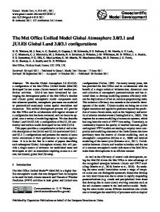
Fig. 8. Comparisons of model simulation and predictions using Taylor series expansions for concentrations of nitrate at 16:00 EDT on 2 January 2004, with (a) a 50 % reduction in NOx and (b) a 50 % reduction in SO2 . The solid lines reflect the linear regression of the Taylor series predictions against the CMAQ simulation results; the dotted lines represent the area of perfect agreement.
Geosci. Model Dev., 5, 355–368, 2012
www.geosci-model-dev.net/5/355/2012/
W. Zhang et al.: Development of the high-order decoupled direct method in three dimensions
365
Fig. 9. Comparisons of model simulation and predictions using Taylor series expansions with HDDM and BF sensitivities for concentrations of nitrate with (a) 20 % and (b) 100 % reductions in domain-wide SO2 emissions rates and concentrations of sulfate with (c) 20 % and (d) 100 % reductions in domain-wide NH3 emissions rates at 16:00 EDT on 2 January 2004. BF sensitivities are from a 50 % perturbation. The solid lines reflect the linear regression of the Taylor series predictions against the CMAQ simulation results; the dotted lines represent the area of perfect agreement.
Therefore, the time required by matrix factorization and transport-related computations is almost the same for firstand second-order sensitivities. An indirect cost associated with the second-order sensitivity calculation is that all relevant first-order sensitivities should also be calculated, which is generally of interest anyway in any application involving high-order sensitivity (Hakami et al., 2003). On the other hand, BF needs more than one simulation, and its computational cost increases directly with the order and the number of sensitivity parameters. HDDM-3D/PM provides an efficient approach to conduct high-order sensitivity analysis as it computes high-order sensitivities at a similar computational effort as first-order sensitivities. HDDM-3D/PM has many practical applications, most of which are based on Taylor series expansion (Hakami et al., 2003): C(1ε) = C(0) + 1εS (1) (0) +
1ε2 (2) S (0) + higher order terms 2
www.geosci-model-dev.net/5/355/2012/
(17)
where C(0) stands for the pollutant concentration at base case emissions and C(1ε) with a perturbation of 1ε in emissions. With Eq. (17), one can quickly compute the impact of emission perturbations on the ambient concentrations of pollutants. Including the second-order term (i.e., the third term on the right hand side of Eq. (17)) is expected to reduce the error between the approximations using Taylor series expansion and the model simulation. For example, assuming 50 % of domain-wide NOx emissions are reduced in the simulation above, we predicted the concentration of nitrate using first- and second-order Taylor series expansion (Eq. (17)) and compared them with model simulation (Fig. 8a). Predictions using second-order Taylor series expansions are closer to the model simulation than those using first-order Taylor series expansions (Fig. 8a). A similar result is also found for nitrate concentration with a 50 % reduction in SO2 emissions (Fig. 8b). Thus, including the second-order term in Taylor series approximation improves the accuracy of prediction.
Geosci. Model Dev., 5, 355–368, 2012
366
W. Zhang et al.: Development of the high-order decoupled direct method in three dimensions
Taylor series expansions derived using HDDM sensitivity coefficients enable efficient evaluation of emission control strategies. One CMAQ-HDDM simulation would be sufficient to estimate the changes in pollutant concentrations with respect to emission reductions. Predictions of nitrate concentrations with 20 % and 100 % reductions in total SO2 emission using HDDM sensitivities compare well with the CMAQ model simulation. The slope from linear regression analysis is close to 1 (Fig. 9a and b). Predictions driven by BF sensitivities are close to the CMAQ simulation at 20 % reductions and are a little off the one-to-one line for 100 % reductions (Fig. 9b). The BF sensitivities used here are results of a 50 % perturbation. BF sensitivities prepared using a 10 % perturbation were also tested (not shown here), but suffered from more numerical noise. Simulated sulfate concentrations with 20 % and 100 % reductions in total NH3 emissions also exhibit good agreement with model simulation (Fig. 9c and d). The reduction in concentrations that would occur if the sources of interest did not exist is called the zero-out source contribution (ZOC) (Cohan et al., 2005). The advantage of using Eq. (17) to calculate ZOC is that it is based on an air quality model with relevent physical and chemical processes included. Indirect effects, such as source contributions of SO2 emissions to nitrate and NH3 emissions to sulfate (Fig. 9b and d), can be reasonablely evaluated. The ZOC can also be applied to a combination of source emissions. Consider two emission sources (pj and pk ) that are perturbed simultaneously. The expression of ZOC of species i (ZOCi ) can be obtained from Eq. (17) with multiple sensitivity parameters: (1)
(2)
(1)
(2)
(2)
ZOCi (pj ,pk ) ≈ (Si,j − 0.5Si,j,j ) + (Si,k − 0.5Si,k,k ) − Si,j,k
(18)
The cross sensivitity, the last term on the right-hand-side of Eq. (18), is able to quantify the interactions between the two emissions. 5
Conclusions
The high-order decoupled direct method in three dimensions for particulate matter (HDDM-3D/PM) has been implemented in the Community Multiscale Air Quality (CMAQ) model. The implementation of HDDM-3D/PM into ISORROPIA applied a case-specific approach and explicitly computes the sensitivity of activity coefficients. Comparisons of the results with the traditional BF approach generally give good agreement. The BF sensitivities are found to be dependent on the perturbation sizes and the model accuracy, which leads to noisy behavior, especially for high-order sensitivities (Figs. 3 and 7). The direct assessment of second-order sensitivities with HDDM-3D/PM avoids the apparent pitfalls of the BF approach that cause this noise. HDDM-3D/PM has similar computational cost to the previous DDM-3D/PM. The CPU time required by the aerosol Geosci. Model Dev., 5, 355–368, 2012
module to conduct a one-day simulation with one first-order and one second-order sensitivity parameter are 9 and 11 min, respectively. This is another advantage over the BF approach, for which computational time increases more with the order of the sensitivities computed. The implementation of HDDM-3D/PM provides a powerful extension to the CMAQ model, as allowing efficient assessment of control strategy effectiveness, source contribution quantification, and model uncertainty analysis. Initial studies show that Taylor series expansions with the secondorder term predict the model response to various emission levels very well. HDDM-3D/PM can be easily implemented into other versions of CMAQ, as well as other chemical transport models that already include DDM. Supplementary material related to this article is available online at: http://www.geosci-model-dev.net/5/355/2012/ gmd-5-355-2012-supplement.pdf. Acknowledgements. This research was made possible by funding from Conoco-Phillips Inc. and US EPA (Grant numbers: RD83215910, RD83362601, RD83096001, RD82897602, and RD83107601). Edited by: K. Gierens Disclaimer. The contents of this publication are solely the responsibility of the grantee and do not necessarily represent the official views of the US EPA. Further, US EPA does not endorse the purchase of any commercial products or services mentioned in the publication.
References Ansari, A. S. and Pandis, S. N.: Response of inorganic PM to precursor concentrations, Environ. Sci. Technol., 32, 2706–2714, 1998. Ansari, A. S. and Pandis, S. N.: Water absorption by secondary organic aerosol and its effect on inorganic aerosol behavior, Environ. Sci. Technol., 34, 71–77, 2000. Bergin, M. S., Russell, A. G., Odman, M. T., Cohan, D. S., and Chameldes, W. L.: Single-Source Impact Analysis Using ThreeDimensional Air Quality Models, J. Air Waste Manag. Assoc., 58, 1351–1359, 2008. Binkowski, F. S. and Roselle, S. J.: Models-3 community multiscale air quality (CMAQ) model aerosol component – 1. Model description, J. Geophys. Res.-Atmos., 108, 4183, doi:10.1029/2001JD001409, 2003. Boylan, J. W., Odman, M. T., Wilkinson, J. G., Russell, A. G., Doty, K. G., Norris, W. B., and McNider, R. T. : Development of a comprehensive, multiscale “one-atmosphere” modeling system: application to the Southern Appalachian Mountains, Atmos. Environ., 36, 23, 3721–3734, 2002. Bromley, L. A.: Thermodynamic properties of strong electrolytes in aqueous solutions, AIChE J., 19, 313–320, 1973.
www.geosci-model-dev.net/5/355/2012/
W. Zhang et al.: Development of the high-order decoupled direct method in three dimensions Byun, D. and Schere, K. L.: Review of the Governing Equations, Computational Algorithms, and Other Components of the Models-3 Community Multiscale Air Quality (CMAQ) Modeling System, Appl. Mech. Rev., 59, 51–77, 2006. Capps, S. L., Henze, D. K., Hakami, A., Russell, A. G., and Nenes, A.: ANISORROPIA: the adjoint of the aerosol thermodynamic model ISORROPIA, Atmos. Chem. Phys., 12, 527–543, doi:10.5194/acp-12-527-2012, 2012. Carlton, A. G., Bhave, P. V., Napelenok, S. L., Edney, E. D., Sarwar, G., Pinder, R. W., Pouliot, G. A., and Houyoux, M.: Model representation of secondary organic aerosol in CMAQv4.7, Environ. Sci. Technol., 44, 8553–8560, 2010. Carter, W. P. L.: Documentation of the SAPRC99 chemical mechanism for VOC and reactivity assessment, Air Pollution Research Center and College of Engineering, Center for Environmental Research and Technology, University of California, Riverside, CA, 2000. CEP: Sparse Matrix Operator Kernel Emissions Modeling System (SMOKE) User manual; Carolina Environmental Program, 2003. Cohan, D. S., Hakami, A., Hu, Y. T., and Russell, A. G.: Nonlinear response of ozone to emissions: Source apportionment and sensitivity analysis, Environ. Sci. Technol., 39, 6739–6748, 2005. Cohan, D. S., Koo, B., and Yarwood, G.: Influence of uncertain reaction rates on ozone sensitivity to emissions, Atmos. Environ., 44, 3101–3109, 2010. Dunker, A. M.: The Decoupled Direct Method For Calculating Sensitivity Coefficients in Chemical Kinetics, J. Chem. Phys., 81, 2385–2393, 1984. ENVIRON: Users’ Guide, Comprehensive Air Quality Model with Extensions (CAMx), Version 4.20; ENVIRON International Corporation, 2005. Edney, E. O., Kleindienst, T. E., Lewandowski, M., and Offenberg, J. H.: Updated SOA chemical mechanism for the Community Multi-Scale Air Quality model, EPA 600/X-07/025, US EPA, Research Triangle Park, NC, 2007. Fountoukis, C. and Nenes, A.: ISORROPIA II: a computationally efficient thermodynamic equilibrium model for − K+ Ca2+ Mg2+ NH4+ Na+ SO24 -NO− 3 Cl H2 O aerosols, Atmos. Chem. Phys., 7, 4639–4659, doi:10.5194/acp-7-4639-2007, 2007. Galloway, T. S., Brown, R. J., Browne, M. A., Dissanayake, A., Lowe, D., Jones, M. B., and Depledge, M. H.: A multibiomarker approach to environmental assessment, Environ. Sci. Technol., 38, 1723–1731, 2004. Grell, G., Dudhia, J., and Stauffer, D.: A description of the FifthGeneration Penn State/NCAR Mesoscale Model (MM5), NCAR, NCAR/TN 398+STR, 1994. Hakami, A., Odman, M. T., and Russell, A. G.: High-order, direct sensitivity analysis of multidimensional air quality models, Environ. Sci. Technol., 37, 2442–2452, 2003. Hakami, A., Odman, M. T., and Russell, A. G.: Nonlinearity in atmospheric response: A direct sensitivity analysis approach, J. Geophys. Res.-Atmos., 109, D15303, doi:10.1029/2003JD004502, 2004.
www.geosci-model-dev.net/5/355/2012/
367
Kaiser, J.: Mounting evidence indicts fine-particle pollution, Science, 307, 1858–1861, 2005. Kelly, J. T., Bhave, P. V., Nolte, C. G., Shankar, U., and Foley, K. M.: Simulating emission and chemical evolution of coarse seasalt particles in the Community Multiscale Air Quality (CMAQ) model, Geosci. Model Dev., 3, 257–273, doi:10.5194/gmd-3257-2010, 2010. Koo, B., Dunker, A. M., and Yarwood, G.: Implementing the decoupled direct method for sensitivity analysis in a particulate matter air quality model, Environ. Sci. Technol., 41, 2847–2854, 2007. Koo, B., Wilson, G., and Yarwood, G.: High-order Decoupled Direct Method (HDDM) Radical Output Improvements in the Comprehensive Air-quality Model with Extensions (CAMx), 582-784005-FY10-27, 2010. Mendoza-Dominguez, A. and Russell, A. G.: Iterative inverse modeling and direct sensitivity analysis of a photochemical air duality model, Environ. Sci. Technol., 34, 4974–4981, 2000. Napelenok, S. L., Cohan, D. S., Hu, Y. T., and Russell, A. G.: Decoupled direct 3D sensitivity analysis for particulate matter (DDM-3D/PM), Atmos. Environ., 40, 6112–6121, 2006. Nenes, A., Pandis, S. N., and Pilinis, C.: ISORROPIA: A new thermodynamic equilibrium model for multiphase multicomponent inorganic aerosols, Aquat. Geochem., 4, 123–152, 1998a. Nenes, A., Pilinis, C., and Pandis, S. N.: Continued Development and Testing of a New Thermodynamic Aerosol Module for Urban and Regional Air Quality Models, Atmos. Environ., 33, 1553–1560, 1998b. Odman, M. T. and Ingram, C. L.: Multiscale Air Quality Simulation Platform (MAQSIP): Source code documentation and validation, Environmental Programs, North Carolina Supercomputing Center, Research Triangle Park, NC, 1996. Odman, M. T., Boylan, J. W., Wilkinson, J. G., Russell, A. G., Mueller, S. F., Imhoff, R. E., Doty, K. G., Norris, W. B., and McNider, R. T.: Integrated modeling for air quality assessment: The Southern Appalachians mountains initiative project, Journal De Physique Iv, 12, 211–234, 2002. Odum, J. R., Jungkamp, T. P. W., Griffin, R. J., Forstner, H. J. L., Flagan, R. C., and Seinfeld, J. H.: Aromatics, reformulated gasoline, and atmospheric organic aerosol formation, Environ. Sci. Technol., 31, 1890–1897, 1997. Schell, B., Ackermann, I. J., Hass, H., Binkowski, F. S., and Ebel, A.: Modeling the formation of secondary organic aerosol within a comprehensive air quality model system, J. Geophys. Res.Atmos., 106, 28275–28293, 2001. Seinfeld, J. H. and Pandis, S. N.: Atmospheric Chemistry and Physics: From Air Pollution to Climate Change, 2 ed., Wiley, New York, 2006. Stokes, R. H. and Robinson, R. A.: Interactions in aqueous nonelectrolyte solutions I: Solute-solvent equilibria, J. Phys. Chem.-US, 70, 2126, 1966. Tian, D., Cohan, D. S., Napelenok, S., Bergin, M., Hu, Y. T., Chang, M., and Russell, A. G.: Uncertainty Analysis of Ozone Formation and Response to Emission Controls Using Higher-Order Sensitivities, J. Air Waste Manag. Assoc., 60, 797–804, 2010. US EPA: Air quality criteria for particulate matter, EPA/600/P99/002aF, 2004. Watson, J. G.: Visibility: Science and regulation, J. Air Waste Manag. Assoc., 52, 628–713, 2002.
Geosci. Model Dev., 5, 355–368, 2012
368
W. Zhang et al.: Development of the high-order decoupled direct method in three dimensions
West, J. J., Ansari, A. S., and Pandis, S. N.: Marginal PM2.5 : Nonlinear aerosol mass response to sulfate reductions in the Eastern United States, J. Air Waste Manag. Assoc., 49, 1415–1424, 1999. Yang, Y. J., Wilkinson, J. G., and Russell, A. G.: Fast, direct sensitivity analysis of multidimensional photochemical models, Environ. Sci. Technol., 31, 2859–2868, 1997.
Geosci. Model Dev., 5, 355–368, 2012
Zanobetti, A., Schwartz, J., and Dockery, D. W.: Airborne particles are a risk factor for hospital admissions for heart and lung disease, Environ. Health Perspect., 108, 1071–1077, doi:10.2307/3434961, 2000.
www.geosci-model-dev.net/5/355/2012/