4/18. DFT Theory and Cyclic Convolution. A: Not Necessarily!!!! DFT Theory (Sect
. 7.2.2 in Proakis & Manolakis) tells us: Circular (Cyclic) Convolution. ][*][. ]}[][{.
DFT-Based FIR Filtering See Proakis & Manolakis 7.3
1/18
Motivation: DTFT View of Filtering There are two views of filtering: * Time Domain x[ n ] * Frequency Domain X f (θ )
h[n ]
y[n ] = h[n ] * x[n ]
H f (θ )
Y f (θ ) = H f (θ ) X f (θ )
The FD viewpoint is indispensable for analysis and design of filters: * Passband, Stopband, etc. of |Hf(θ)| * Linearity of Phase ∠Hf(θ), etc. Q: What about using DTFT for implementation? * Compute DTFT of input signal and filter * Multiply the two and take inverse DTFT A: NO!!! Can’t compute DTFT – must compute at infinite many frequency values 2/18
Desired Intention: But Does It Work? But wait…. • If input signal is finite length, the DFT computes “samples of the DTFT” • Likewise, if filter impulse response is finite length Q: So… can we use this? x(0) x(1) : x(N-1)
N-pt DFT
Xf[k]
Hf[k]Xf[k]
N-pt IDFT
Do we get…. y(n) = h[n]*x[n]??
N-pt DFT
h(0) h(1) … h(N-1)
3/18
DFT Theory and Cyclic Convolution A: Not Necessarily!!!! DFT Theory (Sect. 7.2.2 in Proakis & Manolakis) tells us: IDFT{H f [k ] X f [k ]} = h[n ] ⊕ * x[n ] Circular (Cyclic) Convolution
Thus… this block diagram gives something called cyclic convolution, not the “ordinary” convolution we want!!! Q: When does it work??? A: Only when we “trick” the DFT Theory into making circular = linear convolution!!!!!! Q: So… when does Cyclic = Linear Convolution??? Easiest to see from an example!!!!! 4/18
Linear Convolution for the Example What does linear convolution give for 2 finite duration signals: Original Signals: x[n]
Length N1 = 9 n Length N2 = 5
h[n]
n First Non-Zero Output is at n=0: x[n] n h[-n] (flip, no shift – since n=0, multiply and add up) n 5/18
Linear Convolution for the Example (cont.) Last Non-Zero Output is at n = N1 + N2 – 2 = 12: x[n]
(flip, shift by N1 + N2 – 2 = 12, multiply and add up) h[12 - n]
n
n
The non-zero outputs are for n = 0, 1, … , 12 Î 13 of them In General: Length of Output of Linear Convolution = N1 + N2 – 1
6/18
Cyclic Convolution for the Example Now… What does cyclic convolution give for these 2 signals: “Original” Signals:
“First” Output Sample:
1. 2.
Zero-Pad Shorter Signal to Length of Longer One Then Periodize Each
1. 2. 3.
Same as in Linear Conv!!!!
Flip periodized version around this point No shift needed to get n = 0 Output Value Sum over one cycle
Not Present in Linear Conv!!!!
7/18
Linear Convolution for the Example (cont.) “Last” Output Sample (i.e., n = 8): 1. 2. 3.
Flip periodized version around this point Shift by 8 to get n = 8 Output Value Sum over one cycle
Same as in Linear Conv!!!! Note: If I try to compute the output for n = 9 Î Exactly the same case as for n = 0!! Thus, the output is cyclic (i.e., periodic) with unique values for n = 0, 1, …. 8 In General: Length of Output of Cyclic Convolution = max{N1 , N2}
8/18
Making Cyclic = Linear Convolution So…. Some of the output values of cyclic conv are different from linear conv!!! Some of the output values of cyclic conv are same as linear conv And…. The length of cyclic conv differs from the length of linear conv!!!
From the example above we can verify: If we choose K ≥ N1 + N2 – 1 And Zero-Pad Each Signal to Length K Then Cyclic = Linear Convolution
N1 = Length of x[n] N2 = Length of h[n]
Exercise: Verify this for the above example!!!!
9/18
Simple Frequency-Domain Implementation of FIR Filtering X(0)H(0) X(1)H(1) : X(K-1)H(K-1)
x(0) x(1) : x(N1-1) 0 : 0
K-pt IFFT
K-pt FFT
K-pt FFT
Zero-Pad Zero-PadBoth Bothtoto Length LengthKK≥≥NN1+N +N2−1 −1 1
2
If K is Strictly > N1+N2−1 Then there will be extra zeros here that can be ignored y(0) y(1) : : y(K-1)
The TheDFT DFTofof h(n) h(n)isisusually usually Pre-Computed Pre-Computed
h(0) h(1) … h(N2-1) 0 … 0
Why WhyDo DoThis? This? The TheFFT’s FFT’sEfficiency EfficiencyMakes MakesThis ThisFaster Faster Than ThanTime-Domain Time-DomainImplementation Implementation (In (InMany ManyCases) Cases)
10/18
Problems with the Simple FD Implementation Q: What if N1 >> N2? A: Then, need Really Big FFT Î Not Good!!! (Input signal much longer than filter length) Also… can’t get any output samples until after whole signal is available and FFT processing is done. Long Delay. Example: Filter 0.2 sec of a radar signal sampled at Fs = 50 MHz N1 = (0.2 sec)×(50×106 samples/sec) = 107 samples FFT Size > 107 Î Really Big FFT!!!! Q: What if N1 is unknown in advance? Example: Filtering a stream of audio A: FFT size can’t be set ahead of time – difficult programming Simple FD Implementation Has Serious Limitations!!!
11/18
Better FD-Based FIR Filter Implementations Two Very Similar Methods Exist • Overlap – Add (OLA) • Overlap – Save (OLS)
Covered Here
Both methods exploit linearity of filter: • Break input signal into a sum of blocks Î x[n ] = ∑ xi [n ] i • Output = sum of response to each block Ð z[n ] = ( x * h )[n ] =
h )[n ] ∑ (�x� i * �
i
=
= zi [ n ]
∑ zi [ n ]
Use the Simple FD-Based Method to Compute Each Output Block
i
The difference between OLA & OLS lies in how the xi[n] blocks are formed
12/18
OLA Method for FD-Based FIR For OLA: Choose xi[n] to be non-overlapped blocks of length NB (blocks are contiguous)
⎧ x[n ], iN B ≤ n < (i + 1) N B xi [ n ] = ⎨ otherwise ⎩0,
NB is a Design Choice
Q: Now what happens when each of these length-NB blocks gets convolved with the length-N2 filter? A: The output block has length N2+ NB – 1 > NB * Output Blocks are Bigger than Input Blocks “Overlap-Add” * But are separated by NB points * Thus… Output Blocks Overlap * Total Output = “Sum of Overlapped Blocks”
13/18
Figure from Porat’s Book
14/18
OLA Method Steps Assume: Filter h[n] length N2 is specified Choose: Block Size NB & FFT Size NFFT = 2p ≥ NB + N2 – 1 Choose NB such that: NB + N2 – 1 = 2p It gives minimal complexity for method (see below)
Run: Zero-Pad h[n] & Compute NFFT-pt FFT (can be pre-computed) For each i value (“For Each Block”) • Compute zi[n] using Simple FD-Based Method f f f
Zero-Pad xi[n] & Compute NFFT-pt FFT Multiply by FFT of h[n] Compute IFFT to get zi[n]
Overlap the zi[n] with previously computed output blocks • Add it to the output buffer •
15/18
OLA Method Complexity • • • •
The FFT of filter h[n] can be pre-computed Î Don’t Count it! We’ll measure complexity using # Multiplies/Input Sample Use 2NFFTlog2NFFT Real Multiplies as measure for FFT Assume input samples are Real Valued Can do 2 real-signal FFT’s for price of ≈ 1 Complex FFT (Classic FFT Result!)
• For Each Pair of Input Blocks f f f f
One FFT: Multiply DFT × DFT: One IFFT: Total:
2NFFTlog2NFFT Real Multiplies 4NFFT Real Multiplies 2NFFTlog2NFFT Real Multiplies 4NFFT [1 + log2NFFT] Real Multiplies = 4(NB + N2 – 1) [1 + log2(NB + N2 – 1)]
• The Number of Input Samples = 2 Blocks = 2NB • # Multiplies/Input Sample = 2(1 + (N2 – 1)/ NB) [1 + log2(NB + N2 – 1)] 16/18
Comparison to TD Method Complexity Complexity of TD Method •Filter h[n] has length of N2 • To get each output sample: f
Multiply each filter coefficient by a signal sample: N2 Multiplies
• # Multiplies/Input Sample = N2 Multiplies Condition Needed For OLA to Be More Efficient: ⎛ N −1⎞ ⎟⎟[1 + log 2 (N 2 + N B − 1)] < N 2 2⎜⎜1 + 2 NB ⎠ ⎝
Thus… For a given N2, Choose NB to minimize the left-hand side 17/18
FD Complexity vs TD Complexity Plot of: [Left-Hand Side]/[Right-Hand Side] of (5.38) Contours = (OLA Multiplies)/(TD Multiplies)
5
10
4
Block Size N B
10
0.2
2.5
0.4 1
0.6
Optimal Block Size For Filter Length of ≈ 125 (Compare to Table 5.2 in Porat)
0.3
3
10
0.8 1.5
2
10
1
10
20
40
60
80 100 120 Filter Length N2
OLA More Efficient Only For Filters Longer than 19
140
160
180
200
18/18