1574
J. Opt. Soc. Am. A / Vol. 25, No. 7 / July 2008
Shioiri et al.
Differences in temporal frequency tuning between the two binocular mechanisms for seeing motion in depth Satoshi Shioiri,1,* Tomohiko Nakajima,2 Daisuke Kakehi,2 and Hirohisa Yaguchi2 1
Research Institute of Electrical Communication, Tohoku University, 2-1-1, Aoba-ku, Sendai, 980-8577 Japan 2 Department of Information and Image Sciences, Chiba University, 1-33, Inage-ku, Chiba, 263-8522 Japan *Corresponding author:
[email protected] Received December 10, 2007; revised April 3, 2008; accepted April 17, 2008; posted April 22, 2008 (Doc. ID 90698); published June 9, 2008
There are two types of binocular cues available for perception of motion in depth. One is the binocular disparity change in time and the other is the velocity difference between the left and the right retinal images (interocular velocity differences). We measured the luminance contrast threshold for seeing motion in depth while isolating either of the cues at various temporal modulations of velocity in the stimulus. To isolate disparity cues, dynamic random-dot stereograms were used (the disparity condition) while binocularly uncorrelated random-dot kinematograms were used to isolate velocity cues (the velocity condition). Results showed that sensitivity peaked at a temporal frequency 共⬃1 cps兲 in the velocity condition while the peak in the disparity condition was at the lowest frequency 共0.35 cps兲 or at least at a frequency lower than that in the velocity condition. This suggests that the visual system has different temporal frequency properties for the velocity and disparity cues for motion in depth. © 2008 Optical Society of America OCIS codes: 330.1400, 330.4150, 330.5510.
1. INTRODUCTION The human visual system has more than one mechanism that specializes in detecting motion in depth using different depth cues [1–3]. Among them, disparity change in time (DCT) has been shown to be an important cue because motion in depth can be seen without any explicit monocular cue [4–7]. Another binocular cue for motion in depth has been identified in addition to DCT [2,8–12]. The cue is based on inter-ocular velocity differences (IOVDs). The process that analyzes this cue appears to be different from the one that analyzes DCT. To use disparity cues, the spatial offset between the left and the right images is detected first, and then its change over time is calculated. The inter-ocular velocity cue is constructed by first separately calculating the image velocities of the left and right eyes and then subtracting them. Although some studies showed little influence of IOVD on motion-in-depth perception [9,13] evidence for the existence of the mechanism that detects the IOVD cues has been accumulated [3,10,12,14–20]. For example, Shioiri et al. [12] reported that the observer was able to identify the direction of motion in depth without binocular correlation when there are IOVD cues (even without binocular overlap between the stimulus images). Harris and Watamaniuk [21] showed a critical role of the velocity signal for speed judgments along the line of sight. Brooks and Mather [22] showed different dependencies of sensitivity on eccentricity between disparity detection and motion in depth detection. The physiological mechanism that is responsible for motion in depth is in dispute. Although cells sensitive to motion in depth have been reported in cat and monkey 1084-7529/08/071574-12/$15.00
brains [23–25], such results may be interpreted by the responses of cells sensitive to both disparity and motion [26–28]. We have little knowledge about the use of the different cues in the cells since there is, as far as we know, no study with isolation of each type of cue. To psychophysically investigate visual mechanisms, it is useful to model functional mechanisms in a physiologically plausible way in order to specify the issue of interest. We describe the models here to make clear what we mean by the mechanism sensitive to IOVD and by the one sensitive to DCT. We assume that the mechanism of motion in depth sensitive to disparity cues has inputs from disparity detectors with sensitivity to different depths. Based on the disparity signals, this calculates the DCT. The other mechanism sensitive to velocity cues has inputs from monocular motion detectors at the corresponding retinal locations between the two eyes. This is similar to the process that Beverley and Regan [8] and Cynader and Regan [24] have proposed as a motion in depth detector. Figure 1 depicts a schematic of the model for motion in depth considering receptive field properties of motion and disparity sensitive cells. Figures 1(a) and 1(b) describe the models of IOVD and DCT. Cells with even or odd symmetric receptive fields (RFs) detect luminance contrasts in the retinal images. The results of the contrast detection are used to process motion and disparity signals. In the case of IOVD, the motion signal toward the left or right at each eye is detected by calculating motion energy [29,30], and then the difference between the leftward and rightward motion energies is taken as the motion signal along the horizontal axis (horizontal motion signal). Comparisons of the horizontal motion signals between the eyes © 2008 Optical Society of America
Shioiri et al.
Fig. 1. Models of two types of motion-in-depth processes based on (a) motion energy and (b) disparity energy models at the first stage. The energies are calculated with odd and even symmetric filters (mimicking the RF properties of cortical cells), and no phase signal within the region covered by the filters is available at the stage where either the IOVDs or the DCT is calculated to obtain motion-in-depth signals.
Vol. 25, No. 7 / July 2008 / J. Opt. Soc. Am. A
1575
provide the motion in depth signal (Fig. 1 shows subtraction as an example). In the case of DCT, the disparity signal at a certain moment is detected by calculating the disparity energy [31,32]. The difference between the disparity energies for near and far disparities is taken as the depth signal. The difference in depth signal between times 1 and 2 provides the motion-in-depth signal (subtraction as an example). Note that the cells sensitive to both motion and disparity are not likely to directly contribute to the detection of IOVD since their direction sensitivities to the two eyes are similar [28,33]. They are classified as cells that provide the DCT signals in the model described here. An important feature of the models is that there is no position information within the RF at the stage where the motion or disparity energies are compared to obtain motion-in-depth signals. The velocity system does not have the information of the disparity at each moment, and the disparity process does not have the information of the monocular velocity in the models. Although RF locations can be and perhaps are used to calculate binocular and temporal correspondences in the later stages, such processes do not have to calculate disparities or monocular velocities. The IOVD model in Fig. 1 uses the RF locations to determine the location to compare signals between the two retinal images, and the DCT model also uses the RF locations to sequentially compare the signals obtained. Temporal comparison has to be done at the same location for DCT, which is different from comparing signals from different locations for monocular motion analysis. It should be noted that the second stage of the models shows limitations of the processes; the IOVD process may not be able to detect IOVDs with a change in disparity, and the DCT process may not be able to detect disparity changes with a change in horizontal or vertical position. These two processes are complementary in this sense. Because of the difference in the analysis, the temporal characteristics between the two mechanisms may differ and the two mechanisms may have different roles in seeing motion in depth. The mechanism based on motion can be a faster process than the one that requires a disparity analysis, which is possibly a slow process as has been suggested by a long temporal integration duration [34–41]. Different mechanisms with different temporal tuning curves could compensate each other to cope with a wide variety of stimulation received in the everyday life. This notion may be too simplistic to seriously consider since some studies suggest that the binocular process can be fast [42–44] and the motion process can be slow [45–48]. However, there is an experiment that suggests the different temporal characteristics for the use of the two cues for motion in depth. Shioiri et al. [3] showed an improvement of performance to identify the motion-in-depth direction with an increase in speed when the velocity cue was isolated and showed deterioration of performance when the disparity cue was isolated. This is consistent with the notion that there are two different mechanisms with different temporal characteristics to see motion in depth. In this paper, we compared the temporal characteristics for seeing motion in depth between the conditions with the velocity and the disparity cues. We refer to temporal frequency to cycles of modulation in motion-in-
1576
J. Opt. Soc. Am. A / Vol. 25, No. 7 / July 2008
Shioiri et al.
depth signals rather than luminance variation of the stimulus patterns. Several studies measured temporal frequency tuning for seeing depth and modulating the depth signal in time with stimuli with both the velocity and disparity cues [2,49–53], and the results can be summarized as a temporal frequency tuning with a peak at about 1.5 cps (see a summary in [3]). These experiments suggest that the motion-in-depth process as a whole has a temporally bandpass characteristic, which is similar to that for lateral motion (Tyler [52]). To compare temporal characteristics for each of the two possible mechanisms for motion in depth, we measured contrast sensitivity to see motion in depth as a function of temporal frequency of velocity modulation of motion in depth, isolating either the velocity (IOVD) or the disparity (DCT) cues.
2. GENERAL METHOD To isolate the velocity and disparity cues, we used binocularly uncorrelated random-dot kinematograms (the velocity condition) and dynamic random-dot stereograms (the disparity condition), respectively. After making randomdot stereograms moving in depth, the correlation between the eyes (binocular correlation) was randomized in the velocity condition, and the correlation between the frames (temporal correlation) was randomized in the disparity condition. Unfortunately, the isolation of the two cues is not perfect. Random disparity correspondences in binocular uncorrelated patterns may determine the threshold in the velocity condition by stimulating the disparity sensitive mechanism [9,54]. Similarly, random temporal correspondences in dynamic random-dot stereograms may determine the threshold in the disparity condition by stimulating the velocity sensitive mechanism. To show that there are available DCT cues in the velocity condition and available IOVD cues in the disparity condition, we calculated correlations of stimulus images in the possible IOVD and DCT processes. The stimuli were two pairs of random-dot stereograms that disparity changed from back to front of the fixation plane by replacing each other (the left and the right images of frame 1 become the right and the left images of frame 2). Calculating correlation between the left and the right images of random-dot stereograms gives a value that shows similarity of the images so that correlation with the displacement that corresponds to the given disparity is expected to be the largest. Correlation values with a variety of displacements in variable directions construct an image with a peak at a location that corresponds to the displacement (or disparity) between the left and the right images. In the velocity condition, the correlation image of each frame pair becomes a random-dot-like pattern since binocular correlation is removed [not shown but virtually the same as the top two figures in Fig. 2(a)]. However, calculating the correlation between the resultant correlation images for frames 1 and 2 shows a clear peak at a location, which corresponds to the motion-in-depth signal added [not shown but virtually the same as the bottom figure in Fig. 2(a)]. The situation is exactly the same for the IOVD process in the disparity condition. The correlation between the two frames in each eye is calculated, and then correlation
Fig. 2. (a) Analysis to show IOVD cues in a temporally uncorrelated random-dot stereogram that disparity changes in time (stimulus in the disparity condition). The correlation image between two frames sequentially presented for each eye (top left and right) and correlation of the correlation images (bottom). The correlation can be demonstrated by free fusing the two top images. Correlation between the left and the right images for each frame pair shows similar results as the top figures in the binocularly uncorrelated kinematograms. Correlation of the two correlation images for two frames shows a similar result as the bottom figure. (b) Simulated responses of IOVD (left) and DCT (right) models depicted in Fig. 1 for the stimuli of the velocity (uncorrelated between the left and the right images) and disparity conditions (uncorrelated between the first and the second images).
of the resultant correlation images for the two eyes is calculated. With disparity cue stimuli, no obvious peak is seen at any displacement for either of the left or the right images [the top two figures in Fig. 2(a)]. However the correlation between the correlation images of the two eyes shows a clear peak at a location, which corresponds to the given motion-in-depth signal [the bottom figure in Fig. 2(a)]. The analysis shows a similar peak correlation for IOVD in the disparity condition and DCT in the velocity condition, which is not surprising because the calculation is essentially identical. Certainly, careful consideration is required to use these stimuli.
Shioiri et al.
Imperfect isolation, however, is not a serious problem in our experiments because our interest is in the difference in temporal characteristics. We estimated the difference in relative contributions of IOVD and DCT to motion in depth between the two stimulus conditions using the models in Fig. 1. Stimuli were two pairs of random-dot stereograms whose disparity changed from back to front of the fixation plane by replacing each other, as in the case for the correlation analysis above. In the stimulus, upper and lower halves of the stimulus field had opposite disparity to contrast the results between the opposite motion signals. We simulated outputs of the models in Fig. 1 as follows. After calculation of motion and disparity energy to the two frame random-dot patterns, simple subtraction was taken to estimate the motion-in-depth signal in each model, and the resultant images are shown in Fig. 2(b). Figure 2(b) shows the output images averaged over the data for ten different random patterns, but the results from each set of patterns are essentially the same. The pixels lighter than average gray indicate approaching motion and those that are darker indicate receding motion. To the disparity stimulus, only the DCT output shows a clear difference, whereas only the IOVD output shows a clear difference to the velocity stimulus. This analysis shows that the removal of correlation from images should weaken, if not eliminate, the IOVD and DCT signals in
Vol. 25, No. 7 / July 2008 / J. Opt. Soc. Am. A
1577
the disparity conditions. This supports the assumption that the relative strength of the two signals is different in the two conditions. We believe, therefore, that the use of the velocity and disparity conditions are appropriate for our purpose, which is to find the differences in temporal characteristics among the different stimulus conditions. Note that the models did not have any difference in temporal characteristics. Our experimental results can be used to introduce the differences in temporal characteristics in the models of IOVD and DCT in the future. Both the temporal and spatial frequencies of velocity modulation were controlled by varying the velocity of random dots in the stimulus field in space and time (Fig. 3). Temporal or spatial frequency here refers to the number of cycles of periodic velocity change every second and every degree of arc. Note that we manipulated the frequencies of temporal and spatial variations of motion signals, not the variation of luminance contrast, although we manipulated the luminance contrast to measure threshold for motion-in-depth perception. A square wave controlled the velocity variation along the vertical axis, creating a horizontal grating, or a horizontal stack of bands, defined by relative motion signals. The spatial frequency of the grating was fixed to 1 cycle/ image 共0.24 cycles/ deg兲 in experiments 1 and 3 while it varied in experiment 2. We used rotation in depth stimuli in the velocity and
Fig. 3. (a) Schematic of the stimulus for motion in depth at the lowest spatial frequency condition (used in experiments 1 and 3). Left, random-dot planes rotated about the vertical axis without changing the surface direction (always front parallel). The upper and lower halves rotated in the same direction but the phase was opposite. The task in the velocity and combined cue conditions was to discriminate the direction of rotation in depth. Center, random-dot planes oscillated in depth. The phase of the oscillation between the upper and the lower halves was opposite. Right, the random motion noise. Dots distributed within a range of depth moved in random directions. The task in the disparity condition was to discriminate oscillation in depth from the random 3D motion noise. (b) Schematic of the stimuli with different spatial frequencies of velocity modulation (used in experiment 2). A square wave controlled the velocity variation along the vertical axis, creating a horizontal grating, or a horizontal stack of bands, defined by relative motion. The stimulus field was a square of 4.2° ⫻ 4.2°. Dots were always in the square field, wrapping around from one side to the other when dots moved out from the square.
1578
J. Opt. Soc. Am. A / Vol. 25, No. 7 / July 2008
combined cue conditions to eliminate monocular cues in the velocity condition [12,55]. There are monocular cues to identify the direction of motion in depth in the stimulus of linear movement along the depth axis. If the observer could identify the direction of the monocular motion with the knowledge of which eye the signal comes from (eye of origin), he could correctly infer the direction of motion in depth in a linear motion in depth. If the starting location of the rotation is randomized, monocular observation provides no information of rotation directions. In the stimulation, the random-dot pattern rotated in depth about the vertical axis without changing the surface orientation (always front parallel). In other words, all the dots moved in the same way on the screen to generate the same path in the 3D space. When a random-dot stereogram rotated in depth, the stimulus contained both velocity and disparity cues. We used this stimulus as a control (the combined cue condition). To isolate velocity cues (or to minimize the effect of disparity cues), we removed the binocular correlation from the original random-dot stereogram, replacing one of the random-dot patterns with a new one. Since the motion of monocular stimuli was the same as that in the original, the stimulus contained IOVD cues. In this condition, there was little disparity information to form any surface or structure. To isolate disparity cues (or to minimize the effect of velocity cues), we replaced the patterns every second frame while preserving binocular correlations (dynamic random-dot stereograms). Since the disparity was the same as that in the original, the stimulus contained DCT cues. We measured the contrast threshold in each stimulus condition. In the combined cue and velocity cue conditions, the observer responded whether the surface rotated clockwise or counterclockwise when the view was from above (two alternative responses). We adopted a different task in the disparity condition with a two-interval two-alternative forced-choice procedure. A random-dot plane oscillated in depth in one of the two intervals. The motion in the stimulus was the same as that in the combined cue condition except that there were no monocular velocity components because the temporal correlation was removed. In the other interval, dots with random disparities moved around in random directions (random motion noise) within a depth range that corresponded to the moving distance in depth of the oscillation stimulus. Both the oscillation stimulus and the random motion noise appeared to be a similar electronic snowstorm, and there were no clues to discriminate them when monocularly viewed. The observer responded between which of the two intervals contained depth oscillation. The reason why we used this task in the disparity condition was because there would be no information of the rotation direction after removing velocity cues from the original motion-in-depth stimulus. There is a possible criticism of the tasks and stimuli used. The use of different tasks is usually not appropriate to compare absolute sensitivities among conditions. Our purpose, however, was not to compare absolute sensitivities but to compare temporal characteristics. Our assumption is that the task difference does not influence the difference in temporal characteristics between the stimulus conditions. To see the effect of task differences, we
Shioiri et al.
conducted experiment 3, where the same task was used in all conditions, showing similar differences in temporal frequency characteristics to that in experiments 1 and 2.
3. EXPERIMENT 1 The purpose of the experiment was to compare temporal frequency tuning between the velocity and disparity conditions. We measured the threshold of luminance contrast as a function of temporal frequency for direction discrimination of motion in depth. There were two reasons to manipulate the luminance contrast, instead of the motion amplitude, for the threshold measurements. The fast and most important one is to minimize the influence of binocular rivalry. Since binocular rivalry is seldom seen when contrast is lower than 30% for a short stimulus presentation [12,56], the contrast threshold measurements were expected to have little influence on the lack of binocular correlation in the velocity condition. The second reason was rather practical. It was much easier to control the luminance contrast than the motion amplitude at a threshold when the spatial and temporal resolutions of the display systems were considered. A. Method 1. Stimulus The stimuli were random-dot patterns with 1600 light dots on a gray background. Images for the two eyes were presented on two monochromatic monitors (Nanao Flex scan 6500) controlled by a computer (Apple Power Macintosh 7100) separately feeding the red and green signals of the video output to the two monitors. Careful calibration was made measuring the luminance of the center of the stimulus field to realize luminance linearity for each monitor. The maximum luminance of the two monitors was equated by adjusting the luminance control knobs of the monitors. The refresh rate of the system was 67 Hz. The observers viewed the monitors through mirrors arranged to fuse the images at an optical distance of 160 cm. Each random-dot field consisted of 256⫻ 256 pixels that corresponded to 4.2° ⫻ 4.2° in a visual angle. Dot size was 2 ⫻ 2 and dot luminance against the fixed background luminance 共46 cd/ m2兲 was varied to measure the contrast threshold. Contrast refers to Weber contrast, i.e., ⌬L / Lb, where ⌬L is the difference between the dot luminance and the background luminance and Lb is the background luminance. Presentation duration was constant at 0.7 s. The dot velocity sinusoidally varied in time to generate a smooth rotation in depth. There was a 180° phase difference in the rotation between the upper and lower halves (0.24 cycles/ deg condition). Because of the phase difference, one half was at the farthest point when the other was at the nearest point while the rotation direction was the same for both. Temporal frequency (or rotation rate) was either 0.35, 0.7, 1.4, 2.8, 5.6, or 8.4 cps. With the presentation duration of 0.7 s, they corresponded to 0.25, 0.5, 1, 2, 4, or 6 cycles of rotation, respectively. The number of cycles for low temporal frequency stimuli was less than one. We restricted the number of cycles to keep the stimulus presentation duration short and constant in order to minimize
Shioiri et al.
the influence of eye movements. Although the difference in the number of cycles per presentation was a factor that might influence threshold measurements, experiment 3 used the stimulus presentation without temporal limitation to examine any influence on our conclusions. The speed of the moving dots on the display varied with temporal frequency while the temporal frequency of oscillation was not only a factor to determine the speed. The amplitude of both lateral and depth motions also influenced the dot speed. The lateral amplitude was 11 min and the disparity amplitude was 16 min throughout the study. The maximum speed of the lateral motion component, which was the speed at the farthest or the nearest point from the observer (where the depth motion component was zero), varied from 0.4 to 9.7 deg/ s for a temporal frequency change from 0.35 to 8.4 cps (with a lateral motion amplitude of 11 min). The maximum speed of the depth motion component, which was the speed at the fixation plane (where the lateral motion component was zero), varied from 0.3 to 7.1 deg/ s (with a disparity change amplitude of 16 min). The initial phase of the rotation randomly varied from trial to trial among four phases (0°, 90°, 180°, and 270°) for 1.4, 2.8, 5.6, and 8.4 cps and varied between the two (0° and 180°) for 0.35, 0.7, and 1.4 cps. The phases of 0° and 180° corresponded to the nearest and farthest points, and the phases of 90° and 270° corresponded to the points on the fixation plane. The measurements with 1.4 cps were repeated to examine whether there was any influence of the number of initial phases. We pooled the data with four and two initial phases in the 1.4 cps conditions since the results were almost the same in the two cases.
2. Procedure and Observers Each trial started with the presentation of nonius lines and a fixation cross. The nonius stimulus consisted of horizontal and vertical lines presented either left and above or right and below the fixation cross. The observer pressed a key to initiate the stimulus presentation when he confirmed the alignments of the horizontal and vertical lines. In the velocity and combined cue conditions, the stimulus rotated for 0.7 s and the observer pressed either of two keys to indicate the perceived direction of rotation (clockwise or counterclockwise). In the disparity condition, the oscillation in the depth and random motion stimuli were presented in sequence for 0.7 s each, with a 0.5 s of blank field in between. The observer responded to the interval during which oscillation in depth was seen. The experiment repeated trials varying stimulus contrast with the method of constant stimulus. We determined the contrast with 75% correct responses as the threshold in each condition through a probit analysis based on 288 or occasionally more trials. Two of the authors and two experienced observers who were naive to the purpose of the experiment participated. All observers had normal or corrected to normal visual acuity and no history of any vision related diseases. Binocular stereopsis was checked with a high contrast version of static random-dot stereograms. All observers had a few practice sessions with feedback to become accustomed to the stimuli and the task.
Vol. 25, No. 7 / July 2008 / J. Opt. Soc. Am. A
1579
B. Results Figure 4 shows the percentage of correct responses as functions of the stimulus contrast in the three motion conditions for 0.7 cps of one observer as examples. Figure 5 shows contrast sensitivity for detecting motion in depth signals as a function of temporal frequency for the three stimulus conditions. Since a different task was used in the disparity condition from the others, it is not appropriate to compare absolute sensitivities between the conditions. However, our interest is in the frequency tuning curves. Differences in temporal frequency tuning between the velocity and disparity conditions are clearly shown. The result in the velocity condition showed a bandpass characteristic of the frequency function while the disparity condition shows a low-pass characteristic in the averaged data. These tendencies are also seen in the individual results. Although lower temporal frequencies may be required to estimate the shape of the tuning function in the disparity condition, differences in frequency dependency are clearly seen among the conditions. Sensitivity in the combined cue condition is similar to but somewhat higher than that in the velocity condition at all frequencies. To examine whether the dependency of sensitivity on temporal frequency is different between the velocity and disparity conditions, a statistical test was performed for the significance of the correlation between the data. We calculated a correlation coefficient between the data pairs of each combination of the three conditions. The number of the available data was less than 6 (temporal frequencies) ⫻5 (observers) and varied with combinations because threshold was not measurable in some cases. For the sake of fair comparison, we used data when they were available from all three conditions. The test showed that the correlation is not statistically significant between the velocity and disparity conditions 共t = 1.56, df = 15, p ⬎ 0.1兲 while the correlation between the velocity and combined cue conditions is highly significant 共t = 10.0, df = 15, p ⬍ 0.001兲. The correlation between the combined cue and disparity conditions is not significant 共t = 1.03, df = 15, p ⬎ 0.3兲. These results suggest that there are two different mechanisms with different temporal frequency tuning curves for seeing motion in depth in the velocity and disparity conditions. The sensitivity in the combined cue condition may be attributed to a combined activity of the two mechanisms. If this is the case, the present results
Fig. 4. Percentages of correct responses as a function of contrast for three motion-in-depth stimulus conditions at 0.7 cps of observer DK. The curves indicate the cumulative Gaussian functions fitted to the data through a probit analysis.
1580
J. Opt. Soc. Am. A / Vol. 25, No. 7 / July 2008
Fig. 5. Contrast sensitivity as a function of temporal frequency. Different symbols represent different stimulus conditions. Error bars for the average data represent the standard error of means across the observers. Arrows indicate conditions where threshold was not measurable.
Shioiri et al.
B. Results and Discussions Figure 6 shows the contrast sensitivity as a function of temporal frequency in the different spatial frequency conditions. As in experiment 1, our interest is in frequency tuning instead of absolute sensitivity. The results confirmed that the temporal frequency characteristic is different between the velocity and disparity conditions. In the velocity condition, the sensitivity data show a bandpass tuning with a peak at about 1 cps except for observer TN at 1.9 cycles/ deg. In the disparity condition, the sensitivity data show a low-pass characteristic except for observer TN at 0.95 cycles/ deg. The same statistical test as that in experiment 1 was performed to examine whether the dependency of sensitivity on temporal frequency is different between the velocity and disparity conditions. We calculated a correlation coefficient for the data pairs averaged over spatial frequencies to focus on the effect of temporal factors. The test showed that the correlation is not statistically significant between the velocity and disparity conditions although it is close to the significant level of 5% 共t = 2.28, df = 5 , p ⬎ 0.05兲. In contrast, the correlation between the velocity and combined cue conditions is highly significant 共t = 9.72, df = 5 , p ⬍ 0.0002兲. The correlation between the combined cue and the disparity conditions is not significant although it is close to the significant level
suggest that the influence of the mechanism sensitive to velocity cues is strong in the present condition because the sensitivity in the combined cue condition is similar to that in the velocity condition.
4. EXPERIMENT 2 Results of experiment 1 suggest that in different stimulus conditions there are differences in temporal characteristics for seeing motion in depth. To examine the generality of this finding with respect to spatial conditions, we repeated the sensitivity measurements with variable spatial frequencies in experiment 2. The dot motion varied along the vertical axis, following a square wave, and the frequency of the square wave was either 0.24, 0.48, 0.95, or 1.9 cycles/ deg [Fig. 2(b)]. For higher spatial frequencies, the stimulus contained a larger number of bands. A. Method In experiment 2, we collected contrast sensitivity data with the combinations of three spatial and six temporal frequencies for two observers, and they are analyzed together with the results of experiment 1. The method was the same as in experiment 1 with one exception in the stimulus. Horizontal lines were added at the borders between adjacent bands in this experiment. This was to minimize vertical eye misalignments. Without the lines, appropriate binocular fusion might not have been realized in high spatial frequency stimuli, particularly in the velocity condition. The stimulus in the velocity condition had no spatial correlation between the left and right retinal images.
Fig. 6. Contrast sensitivity as functions of temporal frequency for different spatial frequency separately, for three stimulus conditions. The left panels are for TN and the right ones are for KY. The top panels show the results in the velocity condition, the middle in the disparity condition, and the bottom in the combined cue condition. Error bars indicate the standard error of means obtained through a probit analysis. Error bars are not shown when standard error is smaller than the symbol.
Shioiri et al.
of 5% 共t = 2.56, df = 5 , p ⬎ 0.05兲. Although we do not claim that there is no correlation between the disparity and the other conditions, we claim that it is weaker than that between the combined cue and velocity conditions. This is consistent with a two-channel model rather than a singlechannel model, which predicts a similar correlation between all pairs of the three conditions. These results, therefore, confirmed the difference in temporal frequency tuning between the mechanisms that process IOVD and DCT. The effect of spatial frequency is similar among conditions in terms of the reduction of sensitivity for higher spatial frequencies. This general tendency agrees with sensitivity reduction for detailed features defined by motion or disparity [2,49–53]. Another tendency is that sensitivity tuning in the velocity condition is at higher spatial frequencies than that in the disparity condition. The highest sensitivity was found at 0.24 cycles/ deg in the disparity, whereas it was at 0.48 cycles/ deg in the velocity condition. Furthermore, sensitivity is lower in the disparity condition than in the other conditions at high spatial frequencies. This agrees with a recent paper that showed that spatial resolution for speed discrimination of motion in depth was higher with velocity cues than without them [57]. The result suggests that spatial characteristics are also different between the velocity and disparity conditions, and this issue should be fully probed in further investigations.
5. EXPERIMENT 3 Experiment 3 was conducted to examine the effects of two factors that were not controlled in experiments 1 and 2. First, the task in the disparity condition was different from that in the other conditions. We were not concerned with possible sensitivity differences due to task differences since our purpose was to compare the frequency dependencies among different conditions. However, we cannot rule out the possibility that task differences influence the frequency dependency. To avoid the problem, we used the same task in all conditions in experiment 3. Second, we used cycles less than 1 at low temporal frequencies in experiments 1 and 2 to minimize the effect of eye movements. Experiment 3 used a method of adjustments to measure contrast thresholds for seeing motion in depth. The stimulus was the same in the disparity condition as that of the previous experiments. In the velocity and combined cue conditions, the path of motion in depth was a straight line parallel to the head direction rather than rotation in depth. The same oscillation in depth was used in all three conditions. In the velocity condition, the observers reported that they had difficulties extracting motion in depth because they saw lateral motion in addition to motion in depth. They described the lateral motion they saw as either in one direction or a spatial mixture of the two (often dots in the left and right halves were seen moving in opposite directions). Despite the subjective difficulties, they managed to perform the task with a good precision after a few training sessions. In the training sessions, they experienced clear perception of motion in depth with high contrast (but not too high to avoid the influence of binocular rivalry in the velocity condition)
Vol. 25, No. 7 / July 2008 / J. Opt. Soc. Am. A
1581
stimulus. Stimulus temporal frequency was informed before settings in the experimental sessions as well as training sessions. This was to avoid possible confusion between motion-in-depth signals with other temporal factors, particularly in the disparity condition, where replacements of the dots caused continuous transient signals. A. Method In experiment 3, the observers controlled dot contrast so that the motion in depth was just detectable while the stimulus was continuously moving at a given temporal frequency. Because of the long stimulus presentation, we cannot rule out the possible influence of vergence eye movements in this experiment. However, we do not think the effect was serious. Vergence is known to respond without perceiving motion in depth, and relative motion is usually necessary to see motion in depth [58]. We used relative motion stimuli, and the observer’s task was to detect the relative motion in depth between the top and bottom halves. One spatial condition of 0.24 cycles/ deg was used. There were three stimulus conditions and five temporal frequencies (0.31, 0.63, 1.25, 2.5, and 7.5 cps). Two new observers participated in the experiment and ran two sessions of five adjustments in each condition. They had normal or corrected to normal visual acuity, binocular vision, and no history of any vision related diseases. The observers also adjusted the contrast so that the dot pattern was just visible in each stimulus condition to measure the sensitivity of pattern detection. The contrast threshold for static depth in a static random-dot stimulus was also measured with a disparity of 8 min (the top half had a cross disparity and the bottom half had an uncrossed disparity). This experiment used a apparatus similar to the one in experiments 1 and 2. Stimulus was presented on a color monitor (Sony CPD-G500J) controlled by a computer (Apple Power Macintosh G4). The left and right images were presented side by side on the monitor and observed through a mirror stereoscope. Careful calibration was made to realize the output linearity for the monitor. The stimulus size and resolution was the same as in the previous experiments, but the background luminance was 30 cd/ m2 and the display refresh rate was 60 Hz. B. Results and Discussion Figure 7 shows the contrast sensitivity as a function of temporal frequency. The differences between the velocity and disparity conditions are clear. Although the frequency dependencies in the disparity condition are slightly bandpass rather than low pass as in experiment 1, the sensitivity in the disparity condition tends to become higher than that in the velocity condition at lower temporal frequencies. To show this point more clearly, Fig. 8 shows a relative sensitivity between the velocity and disparity conditions (Velocity/Disparity) as a function of temporal frequency for each of the observers of experiments 1 and 3. All observers from the two experimental conditions showed that the ratio increases with temporal frequency, indicating the relative importance of velocity cues at high temporal frequencies. These results confirmed that the two mechanisms with different temporal tuning contribute to seeing motion in depth. The same tendency is seen
1582
J. Opt. Soc. Am. A / Vol. 25, No. 7 / July 2008
Shioiri et al.
Fig. 8. Sensitivity ratio between the velocity and the disparity conditions as a function of temporal frequency for all the observers in experiments 1 and 3.
Fig. 7. Contrast sensitivity as a function of temporal frequency for each stimulus condition in experiment 3, where the same task of detection of motion in depth was used in all stimulus conditions. Error bars indicate standard error of means (not shown when it is smaller than the symbol). The data points with arrows indicate the condition where sensitivity was too low to measure. Open symbols are for pattern detection and filled symbols are for motion in depth. The arrows directed to the left indicate the contrast sensitivity to static display, and the arrows at the horizontal axis indicate that the sensitivity was too low to measure.
for both observers despite the large difference in relative sensitivities between the velocity and disparity conditions. The result in the combined cue condition is interesting. The frequency dependency between the two observers is different. For observer MO, the sensitivity appears to follow the sensitivity of the velocity condition and for observer ST it seems to follow that of the disparity condition in general. However, the sensitivity appears to follow the envelope of the sensitivity functions in the velocity and disparity conditions for both observers if we consider the results at the highest frequency for ST and the lowest frequency for MO. The quick reduction of sensitivity to the disparity cue seems to reveal the use of the velocity cue in
the combined cue condition for ST at the highest frequency. The quick reduction of sensitivity to velocity cue seems to reveal the use of the disparity cue in the combined cue condition for MO at the lowest frequency. The same statistical test was performed to examine whether the dependency of sensitivity on temporal frequency is different between the velocity and disparity conditions. The test showed that the correlation is not statistically significant between the velocity and disparity conditions 共t = 0.75, df = 8 , p ⬎ 0.4兲 while it is significant between the velocity and combined cue conditions 共t = 2.98, df = 8 , p ⬍ 0.02兲. The correlation between the combined cue and disparity conditions is not significant 共t = 0.74, df = 8 , p ⬎ 0.4兲. The result for the individual observer was similar. Correlation was never even close to a significant level between the velocity and disparity conditions for the two observers, and significant correlation was found only between the velocity and combined cue conditions for MO. The correlations between the velocity and disparity conditions, between the velocity and combined cue conditions, and between the disparity and combined cue conditions are 共t = 1.42, df = 3 , p ⬎ 0.2兲, 共t = 0.34, df = 3 , p ⬎ 0.2兲, and 共t = 2.51, df = 3 , p ⬎ 0.08兲 for ST and 共t = 0.21, df = 3 , p ⬎ 0.8兲, 共t = 6.43, df = 3 , p ⬍ 0.01兲, and 共t = 0.51, df = 3 , p ⬎ 0.6兲 for MO. The results for stimulus detection are similar in all three conditions for both observers. Although sensitivity in the disparity condition is slightly lower than those in the other conditions, the large difference in shape of the tuning functions, such as that found for motion in depth, is not seen. The correlation between the data of each pair of the three conditions is significantly different from no correlation (t = 2.46, 2.88, and 2.32 for the velocity versus the disparity, the disparity versus the combined, and the velocity versus the combined, respectively, and df = 3, p ⬍ 0.05 for all). This suggests that the differences in temporal characteristics among conditions for motion in depth cannot be attributed to the difference in stimulus visibility. The results of experiment 3 are consistent with the results in experiments 1 and 2 in general. This confirms the conclusion that there are two different mechanisms with different temporal frequency tuning for motion in depth.
Shioiri et al.
This also indicates that the smaller number of rotation cycles in experiments 1 and 2 was not crucial for the difference in temporal frequency dependency between the velocity and disparity conditions.
6. DISCUSSION The present experiments showed differences in temporal characteristics for seeing motion in depth between the velocity and disparity conditions. Our measurements suggest that the visual system remains sensitive to velocity cues in relatively high temporal frequency stimulations and to disparity cues in relatively low temporal frequency stimulations. We made an additional analysis before drawing conclusions. The correlation analysis above is independent of multiplicative changes of data values, and the analysis is appropriate for the mechanisms with logarithmic coding. Although logarithmic nonlinearity is often assumed in the visual system as a first approximation, it is not necessarily true. Showing the difference in peak frequency is one of the more appropriate ways to show the difference in sensitivity tuning because it is not influenced by changes in absolute sensitivity as long as there is a monotonic relationship between the input and output holds. We estimate the peak frequency of each temporal tuning function from the Gaussian function fitted to the data for each condition of four observers in experiment 1 and two observers in experiment 3. The results showed a clear difference between the velocity and disparity conditions: Average peak frequencies are 0.79, 0.78, and 0.5 for combined cue, velocity, and disparity conditions, respectively. We used a nonparametric test (Wilcoxson sign rank test) to examine whether the differences between the conditions are statistically significant. The test showed the peak difference between the velocity and disparity conditions is statistically significant 共p ⬍ 0.015兲 while it is not between the combined cue and velocity or the disparity conditions (p ⬎ 0.44 or p ⬎ 0.13). We used a nonparametric test because the peaks estimated in the disparity conditions may have relatively large errors because of the lack of data at low frequencies, although the t test showed the same pattern of the results. Based on the experimental results and the above analysis, we claim that two mechanisms with differences in temporal frequency tuning contribute to the perception of motion in depth. The mechanism sensitive to IOVDs tunes to higher temporal frequencies, and the one sensitive to DCT tunes to lower temporal frequencies. There is a different view in the literature from the present one that assumes two motion-in-depth mechanisms sensitive to different temporal frequencies. Cumming and Parker [9] reported little influence of monocular motion signals in a variety of experimental conditions, comparing the threshold of motion amplitude for detecting motion in depth with and without velocity information. These results may suggest that the detection of motion in depth based on IOVDs plays only a secondary role. Harris and Rushton [13] reported experimental results that are consistent with this view. They measured the influence of the stationary noise dots on the velocity threshold of a dot moving in depth and found that stationary
Vol. 25, No. 7 / July 2008 / J. Opt. Soc. Am. A
1583
noise deteriorated the detection of motion in depth. This may imply that threshold for motion in depth is determined by the disparity sensitive mechanism with little contribution of the velocity sensitive mechanism. Our findings of the differences in temporal frequency dependency suggest different roles of the two mechanisms, but it is a different question whether either of the two mechanisms is superfluous in general conditions. If the sensitivity of either one to the stimulation with both cues is independently higher than that of the other of the temporal conditions, the other one may only have a secondary role. Absolute sensitivity with each cue should be compared to answer this question. Although this is not our primary interest and the present experiments were not designed to answer the question, we discuss below some implications of our results. Our results show that sensitivity is higher in the velocity condition than in the disparity condition at a wide range of spatiotemporal frequencies. If we assume that the task difference between the velocity and disparity conditions does not influence the threshold, the results indicate importance of the mechanism to process IOVD in the conditions we used. However, we do not think that it is appropriate to directly compare thresholds between the different conditions and tasks. The comparison between the velocity and combined cue conditions provides more useful information of the relative strength between the disparity and velocity cues. If there was a large contribution of disparity cue in the combined cue condition, the sensitivity should be much higher in the combined cue condition than in the velocity condition. If, on the other hand, there is no contribution of the disparity cue, the sensitivity should be the same in the two conditions. Our results show that the sensitivity in the velocity condition is similar to but somewhat lower than that in the combined cue condition (one exception is the data of ST in experiment 3). In the results of experiment 1, sensitivity in the combined cue condition is never more than twice that in the velocity condition. This indicates that the velocity cues play a nontrivial role in the combined cue condition. The sensitivity difference between the velocity and combined cue conditions can be attributed to the lack of the disparity cue at low temporal frequencies. At low temporal frequencies, sensitivity to disparity is relatively high, and the signal of disparity process is likely to contribute to perception of motion in depth in the combined cue condition. The difference at high temporal frequencies, however, is unlikely to be due to the contribution of the disparity sensitive mechanism. Since the sensitivity reduction at high temporal frequencies in the disparity condition is more severe than that in the other conditions, contribution of the disparity cue should decrease with temporal frequency. One possible interpretation of the sensitivity difference between the conditions at high temporal frequencies is the influence of binocular rivalry. The strength of binocular rivalry depends on the stimulus contrast and little rivalry is seen with contrast lower than 30% when the presentation duration is as short as 0.7 s. Dot contrast is higher than 30% at a threshold at high temporal frequencies in many conditions, and binocular rivalry possibly deteriorates the observer’s performance
1584
J. Opt. Soc. Am. A / Vol. 25, No. 7 / July 2008
at high temporal frequencies as shown in a previous paper using similar stimuli [12]. Absence of binocular rivalry, instead of the addition of disparity signals, could provide an advantage in the combined cue condition over the velocity condition. The above arguments lead us to conclude that sensitivity does not reduce much when the disparity cues are removed and that IOVDs can be the primary source of information to see motion in depth at least in some conditions. Next, we discuss the possible causes of the differences between the previous and present papers. Cumming and Parker [9] and Harris and Rushton [13] showed little influence of velocity cues on perception of motion in depth while the present experiments showed a large influence. The first factor that may cause the differences between the studies is individual variation in relative sensitivities to the velocity and the disparity. It is possible that relative sensitivity differs among different observers and also among different types of sensitivity measurements. For individual variation, there was a report from our laboratory that showed large inter-observer differences in relative sensitivity between the velocity and disparity conditions [58]. The study used stimulus conditions that were the same as those in experiment 1 (0.24 cycles/ deg and 1.4 cps) and measured the contrast sensitivity of 24 naive observers. The results showed that 11 observers were more sensitive to the velocity cue than to the disparity cue while the rest of the observers were more sensitive to the disparity cue. The correlation between the sensitivities in the two stimulus conditions for the observers was analyzed, and the correlation coefficient was found to be 0.29. The low correlation suggested that there are two mechanisms with an independent individual variation in sensitivity. The observers in the present experiments also showed large differences in relative sensitivity between the two stimulus conditions (Figs. 5 and 7). This is also supported by a recent paper that showed an individual variation among stereo blind people in relative sensitivity to the velocity and the disparity [59]. The second factor that may cause the differences between the different studies is the stimulus contrast. We measured the contrast threshold with a fixed amplitude of motion in depth, and the stimulus contrast was lower than 10% in many of the trials. Cumming and Parker [9] and Harris and Rushton [13] measured the thresholds of motion amplitude with high contrast stimuli. The disparity threshold as well as the motion amplitude threshold usually decreases with contrast, but the dependency of threshold on contrast differs among different stimulus conditions [46,60]. The different influences of the stimulus contrast on the sensitivity to the velocity and disparity cues could cause the difference in the relative contribution to motion in depth. Higher amplitude sensitivity in one condition than in the other does not necessarily imply higher contrast sensitivity. The two techniques are complementary to each other in general, but there is an important advantage to measuring contrast threshold in our experiments. With contrast threshold measurements, one can use binocularly uncorrelated random-dot stimuli, minimizing the influence of the binocular rivalry and can also use high speed and/or amplitude stimuli to strongly activate the motion-based mechanism.
Shioiri et al.
7. CONCLUSIONS We measured contrast sensitivity to investigate temporal frequency tuning for velocity modulation in the conditions where either the velocity or disparity cue was isolated. The results showed differences in temporal characteristics between these conditions, suggesting that the two mechanisms with different temporal characteristics contribute to the perception of motion in depth. The two possible mechanisms, perhaps, compensate each other to cope with a wide variety of stimulation received in the everyday situation.
ACKNOWLEDGMENTS This paper was supported in part by grants from Hoso Bunka Kikin and Ministry of Education, Culture, Sports, Science and Technology (MEXT) [Grant-in-Aid for Scientific Research (GASR)-18330153] to S. Shioiri and by the Cooperative Research Project of Research Institute of Electrical Communication (RIEC) at Tohoku University. The authors thank Miho Takeo for her help in collecting data in Experiment 1 and Julian Fernandez for his helpful comments on an earlier version of this paper.
REFERENCES 1. 2. 3.
4.
5. 6. 7. 8. 9. 10.
11. 12. 13. 14.
I. P. Howard and B. Rogers, Binocular Vision and Stereopsis (Oxford U. Press, 1995). D. Regan, “Depth from motion and motion-in-depth,” in Binocular Vision, D. Regan, ed. (MacMillan, 1991), pp. 137–160. S. Shioiri, A. Morinaga, and H. Yaguchi, “Depth perception of moving objects, ” in 3D Television, Video and Display Technology, B. Javidi and F. Okano, eds. (Springer-Verlag, 2002). A. M. Norcia, E. E. Sutter, and C. W. Tyler, “Electrophysiological evidence for the existence of coarse and fine disparity mechanisms in human,” Vision Res. 25, 1603–1611 (1985). A. M. Norcia and C. W. Tyler, “Temporal frequency limits for stereoscopic apparent motion processes,” Vision Res. 24, 395–401 (1984). B. Julesz, Foundations of Cyclopean Perception (University of Chicago Press, 1971). C. V. Portfors-Yeomans and D. Regan, “Cyclopean discrimination thresholds for the direction and speed of motion in depth,” Vision Res. 36, 3265–3279 (1996). K. I. Beverley and D. Regan, “Selective adaptation in stereoscopic depth perception,” J. Physiol. (London) 232, 40P–41P (1973). B. G. Cumming and A. J. Parker, “Binocular mechanisms for detecting motion-in-depth,” Vision Res. 34, 483–495 (1994). M. Maeda, M. Sato, T. Ohmura, Y. Miyazaki, A. H. Wang, and S. Awaya, “Binocular depth-from-motion in infantile and late-onset esotropia patients with poor stereopsis,” Invest. Ophthalmol. Visual Sci. 40, 3031–3036 (1999). D. Regan, “Binocular correlates of the direction of motion in depth,” Vision Res. 33, 2359–2360 (1993). S. Shioiri, H. Saisho, and H. Yaguchi, “Motion in depth based on inter-ocular velocity differences,” Vision Res. 40, 2565–2572 (2000). J. M. Harris and S. K. Rushton, “Poor visibility of motion in depth is due to early motion averaging,” Vision Res. 43, 385–392 (2003). K. R. Brooks, “Monocular motion adaptation affects the perceived trajectory of stereomotion,” J. Exp. Psychol. Hum. Percept. Perform. 28, 1470–1482 (2002).
Shioiri et al. 15. 16. 17. 18. 19. 20.
21. 22. 23.
24. 25. 26. 27. 28.
29. 30. 31. 32.
33. 34. 35. 36.
K. R. Brooks, “Interocular velocity difference contributes to stereomotion speed perception,” J. Vision 2, 218–231 (2002). K. Brooks, “Stereomotion speed perception is contrast dependent,” Perception 30, 725–731 (2001). J. M. Harris and V. F. Drga, “Using visual direction in three-dimensional motion perception,” Nat. Neurosci. 8, 229–233 (2005). J. M. Fernandez and B. Farell, “Motion in depth from interocular velocity differences revealed by differential motion aftereffect,” Vision Res. 46, 1307–1317 (2006). J. M. Fernandez and B. Farell, “Seeing motion in depth using inter-ocular velocity differences,” Vision Res. 45, 2786–2798 (2005). S. Shioiri, D. Kakehi, T. Tashiro, and H. Yaguchi, “Investigating perception of motion in depth using monocular motion aftereffect,” presented at the Vision Sciences Society, Sarasota, Fla., May 13, 2003. J. M. Harris and S. N. Watamaniuk, “Speed discrimination of motion-in-depth using binocular cues,” Vision Res. 35, 885–896 (1995). K. Brooks and G. Mather, “Perceived speed of motion in depth is reduced in the periphery,” Vision Res. 40, 3507–3516 (2000). E. Akase, H. Inokawa, and K. Toyama, “Neuronal responsiveness to three-dimensional motion in cat posteromedial lateral suprasylvian cortex,” Exp. Brain Res. 122, 214–226 (1998). M. Cynader and D. Regan, “Neurons in cat visual cortex tuned to the direction of motion in depth: Effect of positional disparity,” Vision Res. 22, 967–982 (1982). G. F. Poggio and W. H. Talbot, “Mechanisms of static and dynamic stereopsis in foveal cortex of the rhesus monkey,” J. Physiol. (London) 315, 469–492 (1981). Y. Chen, Y. Wang, and N. Qian, “Modeling V1 disparity tuning to time-varying stimuli,” J. Neurophysiol. 86, 143–155 (2001). N. Qian, “Binocular disparity and the perception of depth,” Neuron 18, 359–368 (1997). J. H. Maunsell and D. C. Van Essen, “Functional properties of neurons in middle temporal visual area of the macaque monkey. II. Binocular interactions and sensitivity to binocular disparity,” J. Neurophysiol. 49, 1148–1167 (1983). A. B. Watson and A. J. Ahumada, Jr., “Model of human visual-motion sensing,” J. Opt. Soc. Am. A 2, 322–341 (1985). E. H. Adelson and J. R. Bergen, “Spatiotemporal energy models for the perception of motion,” J. Opt. Soc. Am. A 2, 284–299 (1985). I. Ohzawa, “Mechanisms of stereoscopic vision: The disparity energy model,” Curr. Opin. Neurobiol. 8, 509–515 (1998). I. Ohzawa, G. C. DeAngelis, and R. D. Freeman, “Stereoscopic depth discrimination in the visual cortex: Neurons ideally suited as disparity detectors,” Science 249, 1037–1041 (1990). I. Ohzawa, G. C. DeAngelis, and R. D. Freeman, “Encoding of binocular disparity by complex cells in the cat’s visual cortex,” J. Neurophysiol. 77, 2879–2909 (1997). K. I. Beverley and D. Regan, “Temporal integration of disparity information in stereoscopic perception,” Exp. Brain Res. 19, 228–232 (1974). J. M. Foley and C. W. Tyler, “Effect of stimulus duration on stereo and vernier displacement thresholds,” Percept. Psychophys. 20, 125–128 (1976). R. S. Harwerth and S. C. Rawlings, “Viewing time and
Vol. 25, No. 7 / July 2008 / J. Opt. Soc. Am. A
37. 38. 39. 40. 41. 42.
43. 44. 45. 46. 47. 48. 49. 50. 51. 52. 53. 54. 55. 56. 57. 58. 59.
60.
1585
stereoscopic threshold with random-dot stereograms,” Am. J. Optom. Physiol. Opt. 54, 452–457 (1977). S. Lee, S. Shioiri, and H. Yaguchi, “The effect of exposure duration on stereopsis and its dependency on spatial frequency,” Opt. Rev. 11, 256–264 (2004). K. N. Ogle and M. P. Weil, “Stereoscopic vision and the duration of the stimulus,” AMA Arch. Ophthalmol. 59, 4–17 (1958). R. Patterson, “Spatiotemporal properties of stereoacuity,” Optom. Vision Sci. 67, 123–128 (1990). C. W. Tyler, “Cyclopean vision,” in Vision and Visual Dysfunction, Vol. 9, Binocular Vision, D. Regan, ed. (Macmillan, 1991), pp. 38–74. R. J. Watt, “Scanning from coarse to fine spatial scales in the human visual system after the onset of a stimulus,” J. Opt. Soc. Am. A 4, 2006–2021 (1987). R. Patterson, R. Cayko, G. L. Short, R. Flanagan, L. Moe, E. Taylor, and P. Day, “Temporal integration differences between crossed and uncrossed stereoscopic mechanisms,” Percept. Psychophys. 57, 891–897 (1995). C. W. Tyler, “Binocular cross-correlation in time and space,” Vision Res. 18, 101–105 (1978). W. R. Uttal, N. S. Davis, and C. Welke, “Stereoscopic perception with brief exposures,” Percept. Psychophys. 56, 599–604 (1994). B. Golomb, R. A. Andersen, K. Nakayama, D. I. MacLeod, and A. Wong, “Visual thresholds for shearing motion in monkey and man,” Vision Res. 25, 813–820 (1985). S. Shioiri, S. Ito, K. Sakurai, and H. Yaguchi, “Detection of relative and uniform motion,” J. Opt. Soc. Am. A 19, 2169–2179 (2002). S. Shioiri and P. Cavanagh, “Visual persistence of figures defined by relative motion,” Vision Res. 32, 943–951 (1992). K. Nakayama and C. W. Tyler, “Psychophysical isolation of movement sensitivity by removal of familiar position cues,” Vision Res. 21, 427–433 (1981). S. Nagata, “New versatile stereo (NS-type) disparity system and measurement of binocular depth perception,” J. Jpn. Soc. Med. Electron. Biol. Eng. 20, 154–161 (1982). D. Regan and K. I. Beverley, “Some dynamic features of depth perception,” Vision Res. 13, 2369–2379 (1973). W. Richards, “Disparity masking,” Vision Res. 12, 1113–1124 (1972). C. W. Tyler, “Stereoscopic depth movement: Two eyes less sensitive than one,” Science 174, 958–961 (1971). M. Lages, P. Mamassian, and E. W. Graf, “Spatial and temporal tuning of motion in depth,” Vision Res. 43, 2861–2873 (2003). C. W. Tyler, “Depth perception in disparity gratings,” Nature 251, 140–142 (1974). D. Regan and K. I. Beverley, “Disparity detectors in human depth perception: Evidence for directional selectivity,” Science 181, 877–879 (1973). L. Liu, C. W. Tyler, and C. M. Schor, “Failure of rivalry at low contrast: Evidence of a suprathreshold binocular summation process,” Vision Res. 32, 1471–1479 (1992). K. R. Brooks and L. S. Stone, “Spatial scale of stereomotion speed processing,” J. Vision 6, 1257–1266 (2006). C. J. Erkelens and H. Collewijn, “Motion perception during dichoptic viewing of moving random-dot stereograms,” Vision Res. 25, 583–588 (1985). Y. Watanabe, T. Kezuka, K. Harasawa, M. Usui, H. Yaguchi, and S. Shioiri, “A new method for assessing motion-in-depth perception in strabismic patients,” Br. J. Ophthamol. 92, 47–50 (2008). S. Lee, S. Shioiri, and H. Yaguchi, “Effects of temporal frequency and contrast on spatial frequency characteristics for disparity threshold,” Opt. Rev. 10, 120–123 (2003).