Differential Evolution Algorithm Applied to Non-Stationary Bandit ...

Differential Evolution Algorithm Applied to Non-Stationary Bandit Problem David L. St-Pierre, Jialin Liu

To cite this version: David L. St-Pierre, Jialin Liu. Differential Evolution Algorithm Applied to Non-Stationary Bandit Problem. 2014 IEEE Congress on Evolutionary Computation (IEEE CEC 2014), Jul 2014, Beijing, China. 2014.

HAL Id: hal-00979456 https://hal.inria.fr/hal-00979456 Submitted on 16 Jul 2014

HAL is a multi-disciplinary open access archive for the deposit and dissemination of scientific research documents, whether they are published or not. The documents may come from teaching and research institutions in France or abroad, or from public or private research centers.

L’archive ouverte pluridisciplinaire HAL, est destin´ee au d´epˆot et `a la diffusion de documents scientifiques de niveau recherche, publi´es ou non, ´emanant des ´etablissements d’enseignement et de recherche fran¸cais ou ´etrangers, des laboratoires publics ou priv´es.

Differential Evolution Algorithm Applied to Non-Stationary Bandit Problem David L. St-Pierre

Jialin Liu

University of Li`ege TAO, Inria, Universit´e Paris-Sud, Paris, UMR CNRS 8623, FR B-4000 Li`ege, Belgium 91190 Gif-sur-Yvette, France TAO, Inria, Universit´e Paris-Sud, Paris, UMR CNRS 8623, FR Email: [email protected] 91190 Gif-sur-Yvette, France Email: [email protected]

Abstract—In this paper we compare Differential Evolution (DE), an evolutionary algorithm, to classical bandit algorithms over the non-stationary bandit problem. First we define a testcase where the variation of the distributions depends on the number of times an option is evaluated rather than over time. This definition allows the possibility to apply these algorithms over a wide range of problems such as black-box portfolio selection. Second we present our own variant of discounted Upper Confidence Bound (UCB) algorithm that outperforms the current state-of-the-art algorithms for the non-stationary bandit problem. Third, we introduce a variant of DE and show that, on a selection over a portfolio of solvers for the Cart-Pole problem, our version of DE outperforms the current best UCB algorithms.

I.

I NTRODUCTION

We are interested in a situation where an agent faces K possible options of unknown distribution(s) and is given T sequential evaluations, where T is not necessarily known. The agent is then asked to output π ˜ , a recommendation that corresponds to a probability distribution over K options, according to a performance criterion. In our case the performance criterion is the Simple Regret (SR) and we seek to maximize a reward. This class of problems is well formalized through the bandit framework [1] and more specifically our setting is similar to [2]. Typically this framework tackles effectively the tradeoff between exploration and exploitation. During the evaluation process t ∈ T , the agent selects an option k ∈ K according to its selection policy π(·). A selection policy π(·) ∈ K is an algorithm that selects an option based on the information at hand. A representative example of a selection policy is UCB[3]. At the tth evaluation, the option k is selected and a reward rk,t is computed. A detailed description of the selection policies and the distribution updates used in this paper are provided in Section II. Such a process is repeated until the allocated number of evaluations T has been executed. Afterward, following the recommendation π ˜ , an option k˜ is chosen. The pseudo code for a generic bandit algorithm up to the recommendation of k˜ is provided in Algorithm 1 and the recommendation of k˜ used in this paper is provided in Section II-A. In this paper we focus on non-stationary distributions. A non-stationary bandit problem implies that the distribution of each option k ∈ K changes. In such cases, most of the literature is focused over a

Algorithm 1 Generic Bandit Algorithm. The problem is described through the “get stochastic reward”, a stochastic method and the option sets. The “return” method is formally called the recommendation policy. The selection policy is also commonly termed exploration policy. Require: T > 0: Computational budget Require: K: Set of options Require: π: Selection policy for t = 1 to T do Select k ∈ K based upon π(·) Get stochastic reward rk,t Update the information of k with rk,t end for Return π ˜ : Probability distribution over the set K

variation of distributions based upon the number of evaluations t[4], [5], [6]. In this paper, we focus on a variation based upon the number of times we select an option. The reward distribution for an option improves as we select it more often. Such framework possesses a wide range of applications. The selection of an object from a portfolio is a good example and covers several testcases that justify such a definition. In this paper we are interested in comparing an evolutionary approach, namely Differential Evolution (DE)[7], to the classical bandit approach. DE is arguably one of the main evolutionary algorithms. It does not require heavy computations, performs well on many optimization testbeds [8], [9], [10] and possesses many variants including self-adaptive parameters [11], [12], [13], [14]. Our contribution is a variation of DE that outperforms UCB-Discounted[4] and UCB-Discounted2 (see Section II-A2), both variants of UCB[3] for the non-stationary testcase. Section II formulates the problem and introduces classic selection policies. Section III presents the DE algorithm and our variant. Section IV shows the results and Section V concludes. II.

P ROBLEM S TATEMENT

In this section we formalize the bandit problem and introduce its related selection policy. Section II-A defines the non-stationary problem and presents two variants of UCB, one of the most popular selection policy for stationary bandit,

UCB-Discounted, termed πU CBdt , and our modified UCBDiscounted, termed πU CBdn . These variants of UCB are specific for the non-stationary bandit problem. The first one is designed for problems where the reward distribution changes over time. The second one is a modification that we propose and where the distribution changes over the number of times an option is selected.

2) UCB-Discounted2: We propose a second version of discounted UCB named UCBdn. UCBdn is similar to UCBdt but the discount depends on nk,t , the number of time an option is selected. The idea is still to partially forget past information. The update rule becomes:

r¯k,t =

A. Non-Stationary Bandit Problem In the non-stationary case under study, the reward distribution of the k th option is given by µk,nk,t and represents the expectation of rewards rk,t , where nk,t is the number of times an option k has been selected after the tth evaluation. rk,t is the reward of option k obtained at the tth evaluation and given by ∼ Bernoulli(1, µk,nk,t ), with 1 being the number of Bernoulli trials. At each time t ∈ T the agent chooses an option k ∈ K following a policy π and obtains a reward rk,t . The reward is modeled from distributions unknown to the user. As such, the best option after t evaluations is kt∗ = argmax µk,t . k∈K

The recommendation policy π ˜ usually boils down to selecting the most played option k˜t = argmax nk,t , k∈K

yet there exist several other recommendation policies[15]. We use Simple Regret as optimization criterion. Simple Regret is the difference between the average reward of the best option and the average reward obtained by the recommendation. As we focus on the non-stationary bandit problem, the Simple Regret is thus computed by µkT∗ ,T − µk˜t ,nk,t for t ∈ T . 1) UCB-Discounted: UCBdt[4] is an attempt to adapt UCB to the non-stationary bandit problem. The idea is to partially forget past information. As such, the estimated value computed from rewards is changed from:

r¯k,t = to: r¯k,t =

t P

t P

rki : k i = k

i=1

nk,t

,

(1)

(γ t−i · rki ) : ki = k

i=1 t P

γ t−i

i=1

where γ ∈ (0, 1] and rkt is the reward of the selected option kt obtained at the tth evaluation. Note that if γ = 1 it becomes a UCB as defined for stationary bandit problems. The πUCBdt is given by: s ! ln t(γ) , argmax r¯k,t + C nk (γ) k∈K t P

where C > 0, nk (γ) = γ t−i : ki = k and t(γ) = i=1 P nk (γ). Other padding functions are considered in [5], [16]. k∈K

The main issue in this definition is that the discount depends on t rather than nk,t .

nP k,t

(γ nk,t −i · rki )

i=1 nP k,t

γ nk,t −i

i=1

where γ ∈ (0, 1]. πUCBdn is given by: s ! ln t(γ) argmax r¯k,t + C , nk (γ) k∈K where C > 0, nk (γ) =

nP n,t i=1

III.

γ nk,t −i and t(γ) =

P

nk (γ).

k∈K

D IFFERENTIAL E VOLUTION A LGORITHM

To represent a bandit problem into a framework that can be optimized through an evolutionary approach is far from trivial and is the subject of Section III-A. Section III-B shows the protocol we use for the evaluation of the fitness and Section III-C presents a small variation proposed to greatly improve the performance of DE for bandit problem. Let f : RK → R be the fitness function to be maximized where K is the dimension of the problem. The DE algorithm takes as input a population X of individuals where each individual x ∈ RK are candidate solutions. The goal can be viewed as finding a solution s such that ∀ x ∈ RK f (s) ≥ f (x). Indeed this is for a maximization problem and the solution found is a global maximum. For a minimization, we can easily consider a fitness h : −f instead. The variable t is increased every time a function evaluation is performed. The parameters F ∈ [0, 2], Cr ∈ [0, 1] and |X |, the cardinality of X , have a large impact on the performance of the optimization. Thus, the tuning process is an important part of the algorithm. Algorithm 2 presents our version of the algorithm. A. Representation In our DE algorithm, each individual x ∈ X represents a probability distribution over each option k ∈ K. Obviously, P xk = 1. These individuals are initialized with random k∈K

probabilities as shown in Algorithm 2. Moreover, after each t ∈ T evaluations we keep in memory r¯, a vector of [0, 1]K , representing the different r¯k,t as defined in (1). In this paper, we add r¯ as an individual in X and is updated at the end of each generation. In the following Section we further describe the evaluation of the fitness. B. Evaluation of the fitness When evaluating an individual x, we (i) optionally truncate (see Section III-C) and renormalize, (ii) randomly draw an option k ∈ K (k is selected with probability xk ) and (iii) evaluate the selected option by getting a reward rk,t through t′ Bernoulli trial(s), where t′ > 0 is the number of re-evaluations.

For the evaluation of the fitness f (x), we decide to compute it following X (xk · r¯k,t ). k∈K

Note that xk and r¯k,t are two values accessible without any call to the problem at hand, there is no Bernoulli trial executed during the fitness evaluation. As such, it does not increment the evaluation budget t ∈ T .

focusing on the best options. The rule we used in the algorithm is given by: ( xk if r¯k,t > c1 · max r¯k,t and nk > c2 · max nk,t k∈K k∈K xk = 0 otherwise, where c1 , c2 ∈ (0, 1]. The truncation process is executed during the normalization process when the current number of evaluations is bigger than a given M ≥ 0, as described in Algorithm 2.

Algorithm 2 DE/best/1 Require: K: Dimension Require: T : Computational budget Require: T runcation: 1 if truncated, 0 otherwise Require: M : Threshold if truncated Require: |X |: The size of the population X Initialize each x ∈ X randomly ∈ (0, 1)K Normalize the values xk∈K Initialize t ← 1 Compute f (x) for each x ∈ X Set a : f (a) ≥ f (x) ∈ X while t ≤ T do if T runcation and t > M then Execute truncation end if for each x ∈ X do Evaluate x t′ times t ← t + t′ Pick randomly 2 distinct individuals b and c from X Pick a random index R ∈ K Get a new position y for the individual x as follows: for each k ∈ K do Pick a random number rand ≡ U(0, 1) if rand < Cr or k == R then Set yk = ak + F (bk − ck ) else yk = x k end if end for Normalize the values yk , ∀k ∈ K Compute f (y) if f (y) > f (x) then replace x by y end if if f (x) > f (a) then replace a by x end if end for end while Pick the agent x ˜ ∈ X using recommendation policy Return k˜

IV.

E XPERIMENTS

In this section we describe the various experiments. Section IV-A defines the non-stationary problem at hand, Section IV-B presents the tuning of the UCB variants, Section IV-C shows the tuning of the DE algorithm and finally Section IV-D compares the two algorithms. A. Non-stationary data We use a portfolio of solvers over the benchmark Cart-Pole problem[18] as a testbed. Each option of the bandit problem represents a black-box Direct Policy Search (DPS)[19]. More specifically for our case, we focus on three variants of blackbox Noisy Optimization Algorithms (NOAs) combined with Neural Network (NN) (1, 2, 4, 6, 8 and 16 neurons). The three black-box NOAs are: •

a Self-Adaptive (µ, λ) Evolution Strategy with resamplings (RSAES)[20];

•

a Fabian’s stochastic gradient algorithm with finite differences[21], [22], [23];

•

and a variant of Newton algorithm, adapted for noisy optimization, with gradient and Hessian approximated by finite differences and resamplings[24], termed Noisy Newton.

Basically at iteration n, the NOA chooses one (or more) new point(s) zn in the search domain and gets a reward rk,t . RSAES and Noisy Newton use resamplings, i.e. re-evaluations, to reduce the noise. Note that the budget is consumed accordingly with the number of resamplings. Table I describes the specifics of the NOAs that we use in our experiments. λI represents the number of points selected (more generally termed individuals size) during one iteration, rn is the number of resamplings of each individual and σn is the stepsize. We refer to [25] for more details on the settings and the different algorithms. As shown in Table I, 24 solvers are used to resolve the Cart-Pole problem, thus resulting in 24 options in the nonstationary bandit problem. Experiments are repeated 50 times and we present the mean of these results. B. Tuning of bandit

C. Truncation In order to make DE more competitive, we propose a modification similar in its essence to Bernstein pruning[17]. Since the recommendation π ˜ consists in choosing only one option k˜ and we have access to the current approximation of µk,nk,t through r¯k,t , we can truncate the options that are not likely to be recommended. This ensure that DE is solely

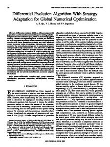
In this section we present the tuning of the different UCBs under study. For the baseline UCB, the only parameter to tune is the C constant, which control the tradeoff between exploration and exploitation. Figure 1 presents a summary of the best combinations of parameters. The x-axis represents the number of evaluations and the y-axis shows the Simple Regret. For each point in Figure 1, 50 independent trials are executed and we present the mean of these results.

TABLE I: Solvers used in the experiments, where d is dimension depending on the number of neurons; rn is resampling number at iteration n for each individual. We refer to [25] for more details. Number of neurons 1, 2, 4, 6, 8, 16 1, 2, 4, 6, 8, 16 1, 2, 4, 6, 8, 16 1, 2, 4, 6, 8, 16

Algorithm and parametrization RSAES with individual size λI = 10d, µ = 5d, rn = 10n2 . Fabian’s solver with individual size λI = 4, stepsize σn = 10/n0.1 , a = 100, no resamplings. Noisy Newton’s solver with individual size λI = 4d2 + 2d + 1, stepsize σn = 10/n, rn = n2 . Noisy Newton’s solver with individual size λI = 4d2 + 2d + 1, stepsize σn = 100/n4 , rn = n2 .

because UCBdt has a forget rate that is not related with the way the distributions evolve its best combination of parameters boils down to almost a normal UCB.

1 C=0.1

0.9

C=1

From Figure 2, it clearly appears that UCBdn is the best variant of UCB for the settings describe in this paper.

0.8 C=2

Simple Regret

0.7 C=20

0.6

C. Tuning of DE In this section we tune different variants of DE and compare them. There are 3 parameters to tune for DE and its variants: λ, F and Cr. Different settings of F ∈ [0, 2] and Cr ∈ [0, 1] are presented in combination with the 2 best population sizes that are found which are λ = 5 and λ = 10.

0.5 0.4

C=200

0.3 0.2 0.1 0 0

UCB−MPA:C=0.1 UCB−MPA:C=1 UCB−MPA:C=2 UCB−MPA:C=20 UCB−MPA:C=200

2

4 6 Number of evaluations

8

10 4

x 10

Fig. 1: Simple Regret for UCB. Tested parameters are C ∈ [10−3 , 200]. For the clarity of graph, we remove some similar results and only show results for C = 0.1, C = 1, C = 2, c = 20 and C = 200. UCBdn converges faster and depends less on C than UCB or UCBdt. The recommendation policy π ˜ is Most Played Arm (MPA), where arm refer to option in our paper.

UCB does not possess the inherent quality to tackle nonstationary bandit problem. Instead, to artificially induce the ability to keep adapting to the variation in the distributions we expect higher exploration rate C. This is exactly what we observe in Figure 1 where the best C constant is 200 when the number of evaluations is below 7×104 and diminishes to 20 as the number of evaluations increases. This value is much higher than on stationary problem where typical empirical values are usually within [0, 2]. For UCBdn and UCBdt, we look for the best combination of parameters C and γ. Figure 2 presents different C values for the best γ = 0.85 found for UCBdn (Top) and the best γ = 0.99 found for UCBdt (Bottom). The rest of the setting is similar to Figure 1. The best combination of parameters for UCBdn seems to be in the vicinity of C = 2 and γ = 0.85 for the given problem. The current γ value indicates that a fair amount of information is lost at each iteration but it is combined with a relatively small exploration factor C = 2. As opposed to UCBdn, UCBdt possesses a very high value for γ and C. Its best γ seems to indicate that UCBdt does not rely on forgetting information throughout the iterations. As such, it is conceivable that it relies on a higher exploration factor C. It appears that

Figure 3 shows average performance of DE in terms of Simple Regret. The x-axis represents the number of evaluations and the y-axis shows the Simple Regret. For each point in Figure 3, 50 independent trials are executed and we present the mean of these results. First, it seems that a smaller population yields better performance. It is understandable since each particle consumes part of the evaluation budget and does not directly share information between them. As such, there is a loss in the efficiency of sampling which increases as the size of the population grows. The best parameter setting for λ = 10 (Bottom) is F = 0.1 and Cr = 0.7, that is a relatively small differential weight F that prevents the distribution to move too fast in a direction but with a relatively high crossover probability Cr. For λ = 5 (Top), the combination F = 0.1 and Cr = 0.7 still yields good results but there exists several other combinations that give similar results. After 9 × 104 evaluations, none of the combination of F and Cr for a λ = 10 reaches a simple regret lower than 0.5 whereas for the same number of evaluations, the combination λ = 5, F = 0.1 and Cr = 0.7 reaches 0.23. Figure 4 presents performance in terms of simple regret for different values of M for the truncated variant of DE presented in Section III-C. We used c1 = 0.7 and c2 = 0.7. The rest of the settings are similar to Figure 3. To facilitate the comparison of performance between normal DE and the truncated variant, we also plot the best normal DE found (λ = 5, F = 0.1, Cr = 0.7). Every tested variant of the truncated version outperform the normal DE. The best truncation factor for a population size λ = 10 appears to be M = 0 which indicates that early truncation are better. From Figure 4, it clearly appears that smaller population size λ yields better results which is in line with previous findings. For a population size λ = 5, the best value of M is 500 in early iterations (< 9 × 104 ) and, as the number of evaluations grows (> 9 × 104 ) the best M is 2 000. These results indicates that truncating early yields good results

1

1

0.9

0.9

0.8

0.8 0.7

C=200

0.6

C=1

0.5 0.4

Simple Regret

Simple Regret

0.7

C=2

C=0.1 C=20

0.3 0.2 0.1

0.6

2

0.1 8

0 0

10 4

F=0.1,Cr=0.4

0.4

0.2

4 6 Number of evaluations

F=0.1,Cr=0.7

0.5

0.3 UCBdn−MPA:C=0.1 UCBdn−MPA:C=1 UCBdn−MPA:C=2 UCBdn−MPA:C=20 UCBdn−MPA:C=200

0 0

F=0.1,Cr=0.1

F=0.1,Cr=0.7 F=0.1,Cr=0.4 F=0.1,Cr=0.1 F=0.4,Cr=0.9 2

x 10

(a) UCB discounted2 (UCBdn) with γ = 0.85.

1

0.9

0.9 C=2

C=1

C=0.1

Simple Regret

Simple Regret

0.6 C=20

0.4

C=200

0.3

0.1

2

4 6 Number of evaluations

0.6 0.5 0.4

0.2 0.1 8

4

F=0.1,Cr=0.7

0.3 UCBdt−MPA:C=0.1 UCBdt−MPA:C=1 UCBdt−MPA:C=2 UCBdt−MPA:C=20 UCBdt−MPA:C=200

0 0

10 x 10

F=0.1,Cr=0.4

0.7

0.5

8

F=0.1,Cr=0.1

0.8

0.7

0.2

4 6 Number of evaluations

(a) Normal DE, λ = 5.

1

0.8

F=0.4,Cr=0.9

10 4

x 10

0 0

F=0.1,Cr=0.7 F=0.1,Cr=0.4 F=0.1,Cr=0.1 F=0.4,Cr=0.9 2

4 6 Number of evaluations

F=0.4,Cr=0.9

8

10 4

x 10

(b) UCB discounted (UCBdt) with γ = 0.99.

(b) Normal DE, λ = 10.

Fig. 2: Top: UCBdn performance with γ = 0.85; Bottom: UCBdt performance with γ = 0.99. Several values of γ and C are tested for UCBdn and UCBdt, we remove some results for the clarity of graphs. Only the best parameterization of γ are presented. UCBdt relies on a higher exploration factor C. UCBdn depends less on C and converges faster than UCBdt using the same constant C.

Fig. 3: Performance of different variants of DE in terms of Simple Regret. Number of options K = 24, population size λ = 5 (Top) and λ = 10 (Bottom). Here we only show a summary of results for the parameters. When F = 0.1, bigger Cr gets better performance. Normal DE can not converge when near to optimum, which is to be expected from an evolutionary algorithm.

yet if the budget is large enough it is better to gather more information before starting the truncation process. D. DE vs Bandit This section compares the best UCBs with the best variants of DE. It is important to note that each algorithm are tuned individually instead of using generic constant for a family of algorithms. In this section, we also add another baseline which consists in choosing an option randomly and always pulling the same one. We call this baseline Random.

Figure 5 shows the average performance in terms of Simple Regret of the best UCBs and DEs. The x-axis represents the number of evaluations and the y-axis shows the Simple Regret. For each point, 50 independent trials are executed and we present the mean of these results. Standard deviation for each curve is of order of magnitude of 0.015. Given a decent number of evaluations, every algorithm outperforms the baseline Random. As expected, the best of the UCB variant (UCBdn) is the best algorithm up to a budget of 5.7 × 104 . Afterward, truncated-DE for λ = 5, M = 500 is

1

1

0.9

0.9

0.8

0.8

0.6 0.5

M=1000

DE

0.4 0.3 0.2 0.1

DE:F=0.1,Cr=0.7 DEt:M=0 DEt:M=500 DEt:M=1000 DEt:M=2000

0 0

2

0.6 DEt:λ=5

0.5 0.4

UCB

UCBdn

0.3 0.2

M=2000

0.1 M=500

4 6 Number of evaluations

8

10

UCBdt DEt:λ=10

2

4 6 Number of evaluations

x 10

0.9

8

10 4

x 10

Fig. 5: Comparison of truncated-DE, UCB, UCBdn, UCBdt and Random. UCBdn outperforms UCB and UCBdt and is clearly the best algorithm if the budget is small. However, as the number of evaluations grows (5.7 × 104 ), truncatedDE gets better (smaller) Simple Regret. Standard deviation for each curve is of order of magnitude of 0.015.

1 DE

0.8 0.7

0 0

Random UCB UCBdn UCBdt DEt:λ=5 DEt:λ=10

4

(a) Truncated-DE compared to normal DE, λ = 5.

Simple Regret

Random

0.7 Simple Regret

Simple Regret

0.7

M=0

M=2000

0.6

V.

C ONCLUSION

0.5

0.3 0.2 0.1 0 0

In this paper, we compare an evolutionary algorithm, namely DE, to bandit algorithms on a black-box portfolio selection problem. Such problems can be formalized into a non-stationary bandit problems, where each option increases their performance as the number of times we evaluate it increases.

M=1000

0.4 DE:F=0.1,Cr=0.7 DEt:M=0 DEt:M=500 DEt:M=1000 DEt:M=2000 2

M=500

4 6 Number of evaluations

M=0

8

10 4

x 10

(b) Truncated-DE compared to normal DE, λ = 10.

Fig. 4: Performance of different variants of DE in terms of Simple Regret. Number of options K = 24, population size λ = 5 (Top) and λ = 10 (Bottom). Here we only show a summary of results for the parameters. Black solid curve is the best DE found in Figure 3. Truncated-DE clearly outperforms the normal DE. M influences slightly on the convergence rate.

the best available algorithm.

There are two important conclusions that we can infer from these experiments. First, the variant of UCB (UCBdn) presented in this paper is the best UCB algorithm for nonstationary bandit problem where the distribution varies with the number of times an option is selected. Second, Evolutionary Algorithm such as DE, given some adaptation, can outperform bandit specific algorithms on bandit problem.

First, we introduce our definition of the non-stationary bandit problem and justify such an approach through a direct application (portfolio of solvers for the Cart-Pole problem). Second, we present the current state-of-the-art bandit algorithms for the given problems and propose our own variant (UCBdn) that outperforms all the other UCB-like algorithm on non-stationary distributions where each distribution changes according to the number of times the option is selected. Third, we introduce DE, an evolutionary algorithm, and apply it over this specific non-stationary bandit problem. We also present our own variant of DE which outperforms the classic version. Fourth and last, we compare the best variant of each category (UCBdn and truncated-DE). If the budget is smaller than 5.7 × 104 we propose the use of UCBdn and, as the number of evaluations increases, truncated-DE is better. For future research, we intend to apply truncated-DE on a wider range of problems. Moreover, we would like to explore the idea of generic parameter tuning in the case of DE. As for the bandit algorithm part, to compute theoretical bound for UCBdn would provide interesting information on its generic performance.

ACKNOWLEDGMENT

[12]

This work is supported by the ADEME POST project. The authors would like to thank the reviewers for their comments.

[13]

R EFERENCES [1] [2]

[3]

[4] [5]

[6]

[7]

[8]

[9]

[10]

[11]

H. Robbins, “Some aspects of the sequential design of experiments,” Bulletin of the American Mathematical Society, vol. 55, 1952. S. Bubeck, R. Munos, and G. Stoltz, “Pure exploration in multi-armed bandits problems,” in Algorithmic Learning Theory. Springer, 2009, pp. 23–37. P. Auer, N. Cesa-Bianchi, and P. Fischer, “Finite-time analysis of the multiarmed bandit problem,” Machine learning, vol. 47, no. 2-3, pp. 235–256, 2002. L. Kocsis and C. Szepesv´ari, “Discounted ucb,” in 2nd PASCAL Challenges Workshop, 2006. J.-Y. Audibert, R. Munos, and C. Szepesv´ari, “Tuning bandit algorithms in stochastic environments,” in Algorithmic Learning Theory. Springer, 2007, pp. 150–165. D. Koulouriotis and A. Xanthopoulos, “Reinforcement learning and evolutionary algorithms for non-stationary multi-armed bandit problems,” Applied Mathematics and Computation, vol. 196, no. 2, pp. 913–922, 2008. R. Storn and K. Price, “Differential evolution–a simple and efficient heuristic for global optimization over continuous spaces,” Journal of global optimization, vol. 11, no. 4, pp. 341–359, 1997. D. Ardia, J. David, O. Arango, and N. D. G. G´omez, “Jump-diffusion calibration using differential evolution,” Wilmott, vol. 2011, no. 55, pp. 76–79, 2011. D. Ardia, K. Boudt, P. Carl, K. Mullen, and B. Peterson, “Differential evolution with deoptim: An application to non-convex portfolio optimization,” The R Journal, vol. 3, no. 1, pp. 27–34, 2011. P. Poa´ık and V. Klema, “Jade, an adaptive differential evolution algorithm, benchmarked on the bbob noiseless testbed,” in Proceedings of the fourteenth international conference on Genetic and evolutionary computation conference companion. ACM, 2012, pp. 197–204. J. Brest, S. Greiner, B. Boskovic, M. Mernik, and V. Zumer, “Selfadapting control parameters in differential evolution: A comparative study on numerical benchmark problems,” Evolutionary Computation, IEEE Transactions on, vol. 10, no. 6, pp. 646–657, 2006.

[14] [15]

[16] [17]

[18] [19] [20]

[21]

[22] [23] [24] [25]

J. Liu and J. Lampinen, “A fuzzy adaptive differential evolution algorithm,” Soft Computing, vol. 9, no. 6, pp. 448–462, 2005. L. S. Coelho and V. C. Mariani, “Combining of chaotic differential evolution and quadratic programming for economic dispatch optimization with valve-point effect,” Power Systems, IEEE Transactions on, vol. 21, no. 2, pp. 989–996, 2006. K. V. Price, R. M. Storn, and J. A. Lampinen, “Differential evolution a practical approach to global optimization,” 2005. C.-W. Chou, P.-C. Chou, C.-S. Lee, D. L. Saint-Pierre, O. Teytaud, M.H. Wang, L.-W. Wu, and S.-J. Yen, “Strategic choices: Small budgets and simple regret,” in Technologies and Applications of Artificial Intelligence (TAAI), 2012 Conference on. IEEE, 2012, pp. 182–187. A. Garivier and E. Moulines, “On upper-confidence bound policies for non-stationary bandit problems,” arXiv preprint arXiv:0805.3415, 2008. V. Mnih, C. Szepesv´ari, and J.-Y. Audibert, “Empirical bernstein stopping,” in Proceedings of the 25th international conference on Machine learning. ACM, 2008, pp. 672–679. A. Weinstein and M. L. Littman, “Bandit-based planning and learning in continuous-action markov decision processes.” in ICAPS, 2012. R. S. Sutton and A. G. Barto, Reinforcement learning: An introduction. Cambridge, MA: MIT Press., 1998. S. Astete Morales, J. Liu, and O. Teytaud, “Noisy optimization convergence rates,” in Proceeding of the Fifteenth Annual Conference Companion on Genetic and Evolutionary Computation Conference Companion, ser. GECCO ’13 Companion. New York, NY, USA: ACM, 2013, pp. 223–224. [Online]. Available: http://doi.acm.org/10.1145/2464576.2464687 V. Fabian, “Stochastic Approximation of Minima with Improved Asymptotic Speed,” Annals of Mathematical statistics, vol. 38, pp. 191– 200, 1967. H. Chen, “Lower rate of convergence for locating the maximum of a function,” Annals of statistics, vol. 16, pp. 1330–1334, Sep. 1988. O. Shamir, “On the complexity of bandit and derivative-free stochastic convex optimization,” CoRR, vol. abs/1209.2388, 2012. S. Astest Morales, M.-L. Cauwet, J. Liu, and O. Teytaud, “Noisy optimization rates,” submitted. M.-L. Cauwet, J. Liu, and O. Teytaud, “Algorithm portfolios for noisy optimization: Compare solvers early,” in Proceedings of the 8th Conference on Learning and Intelligent Optimization, 2014.