Diffusivities and velocity spectra of small inertial particles in turbulent

Downloaded from rspa.royalsocietypublishing.org on April 17, 2012

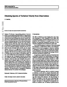
Diffusivities and velocity spectra of small inertial particles in turbulent −like flows J. C. H. Fung, J. C. R. Hunt and R. J. Perkins Proc. R. Soc. Lond. A 2003 459, 445-493 doi: 10.1098/rspa.2002.1023

Email alerting service

Receive free email alerts when new articles cite this article sign up in the box at the top right-hand corner of the article or click here

To subscribe to Proc. R. Soc. Lond. A go to: http://rspa.royalsocietypublishing.org/subscriptions


10.1098/ rspa.2002.1023

Di® usivities and velocity spectra of small inertial particles in turbulent-like ° ows By J. C. H. F u n g1 , J. C. R. H u n t2 a n d R. J. Pe rk i n s3 1

Department of Mathematics, Hong Kong University of Science and Technology, Clear Water Bay, Kowloon, Hong Kong 2 J. M. Burgers Centre, Delft University of Technology, Mekelweg 2, 2628 CD, Delft, The Netherlands and Departments of Space and Climate Physics and Earth Sciences, University College London, Gower Street, London WC1E 6BT, UK 3 Laboratoire de M¶ e canique des Fluides et d’Acoustique, Ecole Centrale de Lyon, 36, Avenue Guy de Collongue, 69134 Ecully Cedex, France Received 9 July 2001; accepted 28 May 2002; published online 6 December 2002

This paper is a study of the random motions of small, spherical inertial particles in spatially and temporarily random turbulent-like velocity elds. The results show how the di¬usivity D p of a small, dense particle depends on the structure of the ®ow eld. The method is to use general, analytical or scaling arguments, model problems and numerical simulations. It is assumed that the particles are so small that the only signi cant forces are inertia, drag and body force, characterized by the relaxation time (½ p ) and the terminal velocity of the particle (VT ). It is shown that only if the ®ow is spatially non-uniform is the di¬usivity of a solid particle D p di¬erent from that of a ®uid particle D f . This small di¬erence, when ½ p is small, is calculated in terms of how the smallest scales contribute to D f and D p . We construct an idealized one-dimensional model consisting of random sets of small èddies’ of length ` separated by a distance of order s with step-like velocity pro les with amplitude u0 (`), superimposed on large-scale eddy motions with length and velocity scales L and U0 , to show the e¬ects of spatio-temporal structure of turbulence on the particle statistics. In order to examine the signi cance of the time dependence of the velocity eld, rstly, the `null’ e¬ect is studied; the velocity eld is `frozen’ in time. It is ~p ¡ D ~ f ) for inertial and ®uid found that the di¬erence between the di¬usivities (D particles, de ned for this narrow range of eddy scales, is of the order of (L`=s)u20 ½ p (for ½ p ½ `=U0 ). Then two unsteady e¬ects are considered. (i) The small eddies are advected by the large-scale motion and move relative to it at a velocity of order ® U0 (where ® ½ 1 ¹ u0 =U0 ); this strength also varies over a time-scale ½ e (¹ `=U0 ). The result is that for larger eddies and smaller ~ p is greater than D ~ f by (L=s)u2 ½ p , particle relaxation times ½ p 6 `=U0 , D 0 where 1 < < U0 =u0 . This increased di¬erence, compared with the frozen turbulence case, is caused by the slower passage of particles through the eddies. (ii) The second unsteady e¬ect is that of eddy decay, so that particles with `suf cient’ inertia do not have time to accelerate within the lifetime of the eddy. Proc. R. Soc. Lond. A (2003) 459, 445{493

445

° c 2002 The Royal Society


J. C. H. Fung and others

446

~ p is less than D ~ f by (L`=s)u0 . By summing over the Then for ½ p & `=U0 , D whole spectrum of eddies in high-Reynolds-number turbulence, the total di¬usivities D p , D f are calculated. It is concluded that for small particle relaxation times (^ ½ p = ½ p U0 =L ½ 1) Dp ¡ D f ¹ Df

¡ ¶

u

(^ ½ p )1=2 + ¶ F

½ ^p ;

where ¶ u , ¶ F are coe¯ cients for the unsteady and structured components. In frozen turbulence and in low-Reynolds-number turbulence without an inertial subrange, ¶ u ’ 0. These order-of-magnitude concepts are used to derive the inertial-range frequency spectra of the velocity of inertial particles ¿ p p (!) and of the ®uid velocity of the locations of the particles ¿ fp (!) in high-Reynoldsnumber turbulence when ½ ^p ½ 1. The predictions are tested and largely con rmed using the technique for kinematic simulation of inertial turbulence. In particular, the prediction is con rmed that D p ¡ D f is negative for the light particle (^ ½ p ½ 1) as the magnitude of the unsteady component of the velocity eld increases and is positive for particles with greater inertia (^ ½ p > 1); in addition, it is shown that the coe¯ cients ¶ u ’ ¶ F ’ 1=3. The e¬ects of particle settling under gravity are also calculated in the idealized model and in the numerical simulation. The results of all the predictions are consistent with the results of direct numerical simulations of particles in three-dimensional turbulence and with some experiments. Keywords: turbulent di®usion; particles and aerosols; multiphase °ows; turbulence simulation and modelling

1. Introduction Recent experimental and computational studies of the motion of small particles in turbulent ®ows have shown how the random displacements X p and velocity p v(t), and their statistical measures such as di¬usivity Dij (where subscripts ì’, `j’ represent di¬erent directions) and mean drift velocity v of particles di¬er from those f and u. These di¬erences depend on the inertia of of the ®uid elements, X f , u(t), D ij the particle and on the drag and body forces FD , FB which act on the particles in the complex space-time structure of the velocity eld. Although these studies have led to several interesting qualitative and statistical results, they have not so far provided any general physical explanation for the e¬ects of turbulence on very small particles. Nor have they led to reliable formulae or simple models for use in practical calculations (at least for parameter ranges where there are small but signi cant di¬erences p f ), because they have not accounted for the relative contributions between Dij and Dij of small- and large-scale turbulence to the di¬erences between D p and D f . To substantiate this strong statement, consider rst the computational results from the direct numerical simulations (DNSs) of Squires & Eaton (1991a) (SE) and from the large-eddy simulations (LESs) of Simonin et al. (1991) (SDM). Both SE and p SDM found that D p (which denotes the magnitude of the tensor Dij or any diagonal p component if Dij is isotropic) is not necessarily equal to D f for inertial particles where FB = 0. In particular, they found that D p > D f and that the di¬erence Proc. R. Soc. Lond. A (2003)


Di® usivities and velocity spectra of small inertial particles

447

increases as the particle inertia increases. In the presence of buoyancy forces, D p is found to exceed D f , and the wind-tunnel experiments of Wells & Stock (1983) showed that D p ¹ D f (to within experimental error) with only inertial e¬ects. Combined with buoyancy e¬ects, the experiment of Snyder & Lumley (1971) showed a marked reduction in D p . In all these cases the turbulent Reynolds number was not high enough to produce a signi cant inertial range in the spectrum. Reeks (1977) and Nir & Pismen (1979), making certain statistical assumptions, concluded theoretically that D p should exceed D f as the relaxation time of the small particle ½ p increases (as a proportion of the integral time-scale TL ). However, other statistical analyses (e.g. Gouesbet et al . 1984) argued that D p = D f . These theories were not explicitly related to the spectra of the particle velocity © p p (!), the velocity as `seen’ by the particle © fp (!). Predictions of these quantities are necessary in order to estimate the dynamical interaction between the particles and the ®uid (e.g. Ooms & Jansen 2000). In the presence of buoyancy forces, Yudine (1959) and Csanady (1963) predicted that the particle di¬usivity D p would decrease, because as the falling particles fall through the eddies, the time-scale of the velocity ®uctuations perturbing their trajectories would be much less than that experienced by ®uid particles moving with the turbulent eddies. However, Squires & Eaton’s (1991a; b) numerical simulations indicated that with a small fall speed VT =U0 , the di¬usivity increases. This needs explaining! In this paper we attempt to provide some qualitative and, in some cases, quantitative answers to the most general unsolved questions about the motion of inertial particles in turbulence. (i) How do the statistics for ®uid and inertial particles vary with the random but ordered space-time structure of the velocity eld for di¬erent values of ½ p =T L ? (ii) How are the di¬erences in the statistics of large-scale e¬ects (e.g. D p relative to D f ) a¬ected by the small di¬erences in the large-scale motions of ®uid and inertial particles (when ½ p =TL ½ 1) as compared with greater di¬erences in their small-scale motions (e.g. spectra at frequencies much greater than TL ¡1 )? In xx 2{4 we estimate, using a one-dimensional model ®ow eld, the magnitudes of the most signi cant mechanisms determining the statistical properties of particle motions in ®ows that vary in time and space. We note that the advection of small-scale eddies by larger eddies (Chase 1970; Tennekes 1975) has a signi cant e¬ect on di¬usion, a mechanism that has been overlooked in previous models of particle motions in turbulence. We also consider the changes in these trends caused by mechanisms that are essentially two- or three-dimensional in nature. Detailed theoretical studies have indicated how various characteristic features of two- and three-dimensional eddy motions have strong e¬ects on particle di¬usion and fall speed (e.g. Squires & Eaton 1991b; Fung 1993, 1997, 1998, 2000; Spelt & Biesheuvel 1997; Davila & Hunt 2001); Lagrangian experiments following particle motions con rmed some of these theoretical observations. The main conclusions are considered in the models presented here, which uniquely indicate how, in ensembles of di¬erent sizes of eddies, the dispersion of particles is a¬ected by the relative spacing, lifetimes and distribution of eddies as much as by their internal structure. Previous simpli ed models have incorporated some but not all of these e¬ects, and therefore have limitations (e.g. Wang & Stock 1993). Proc. R. Soc. Lond. A (2003)



448

Since most hypotheses about the motion of inertial particles (and also of turbulent di¬usion) depend on assumptions about the kinematic structure of turbulence, a good test of these hypotheses and models is to use the technique of kinematic simulation to compute particle motions in di¬erent stationary random ®ow elds that correspond closely to turbulence. The simulations described in x 5 have the same Eulerian spatial and temporal spectra as turbulent ®ows; but, although they do not simulate the nonlinear dynamics of the ®ow eld, such as the interaction between large- and smallscale motion, they appear to simulate the random displacements of ®uid particles, the time-dependent structure of turbulence (for two moments in time) and the spectra of pressure (Fung et al . 1992; Vassilicos & Fung 1995). Since it is not yet possible to simulate a high-Reynolds-number spectrum using DNS over more than one decade (Wang et al. 1996), we cannot yet compute directly how small particles move in a fully developed high-Reynolds-number turbulent ®ow. (Even if the turbulence could be computed, the additional time required to compute particle trajectories would be considerable.) This is why we have had to use kinematic simulation. The results are then considered in terms of the asymptotic limits of either zero fall velocity or very large inertia and are found to be consistent with our theoretical models. We nd signi cant variations in the dependence of D p =D f on ½ p =TL for di¬erent kinds of turbulence. For the appropriate parameters the results of the simulations largely agree with those of experiments and direct numerical simulations. Some of the results derived here were summarized earlier by Hunt et al . (1994).

2. Small particle motion in unsteady non-uniform °ows (a) Equations The velocity v(t) of a particle at X p (t) in a velocity eld de ned by u(x; t) is described by Newton’s second law dv mp = F (u; v; t); (2.1) dt where mp is the mass of the particle. The force F on the particle, which is still the subject of much current research, is made up of many di¬erent contributions, including, for example, the acceleration force FA , the lift force FL , the body force FB and the drag FD (see Mei (1994) or Magnaudet & Eames (2000) for a review of recent developments). If the particle is spherical and if its radius a is small relative to the smallest lengthscale in the turbulence (the Kolmogorov length-scale ² = (¸ 3 =")1=4 ’ 1 mm in the lower atmosphere), then the relative motion approaching a particle is e¬ectively a uniform ®ow. If, also, the particle time constant ½ p is short relative to the shortest time-scales of the velocity eld (½ = (¸ =")1=2 ’ 0:08 s in the atmosphere), and if the Reynolds number based on the relative motion is small enough, then (2.1) reduces to dv = ¡ vR + VT ; (2.2) dt where vR = v(t) ¡ ufp (t) is the velocity of the particle relative to that of the ®uid at the position of the particle, mp g(mp ¡ 43 º a3 » ) ufp (t) = u(X p ; t); ½ p = ; VT = 6º a¸ » 6º a¸ » and g is the acceleration due to gravity. ½

Proc. R. Soc. Lond. A (2003)

p



449

The equation represents a balance of the rate of change of particle momentum caused by its acceleration with the ®uid drag force produced by the motion of the particle relative to the surrounding ®uid and the buoyancy force due to gravity. The major di¯ culty in solving (2.2) is that the independent variable u(X p ; t) is random in space and time. Note that, because dv=dt is not in general parallel to v, even when VT = 0, the trajectories of inertial particles are not, in general, the same as those of ®uid particles starting at the same time. Despite the restrictions that have been imposed, (2.2) is applicable to many di¬erent problems, such as aerosols in gases and small particles in water. (b) Spectra of the ° uid particle and relative velocities Since the equation of motion (2.2) is linear in time, the response v(t) of a particle can be represented as a linear superposition of the response to the Fourier components of ufp (t), de ned using Fourier transforms (see Batchelor 1953) as Z 1 Z 1 e(!)ei!t d! and ufp (t) = e fp (!)ei!t d!; v(t) = v u (2.3) ¡1

¡1

where ! is the circular frequency. Using standard techniques of Fourier analysis, it follows that if VT = 0, then, su¯ ciently long after the release of the particle, v~ (!) =

1 ¡ i½ p ! fp ~ (!): u 1 + ½ p 2!2

If ufp (t) is a stationary random process, the energy spectrum of the particle velocity can be expressed as a function of the energy spectrum of the ®uid velocity along the particle trajectory through a `particle response function’ À (!), which is a measure of the particle response to accelerations or to the frequency spectrum ¿ fpii (!) of the ®uid velocity seen by the particle, i.e. ¿

p p ii

(!) = À

2

(!)¿

fp ii (!);

where À

where the spectra are normalized so that Z 1 fp 2 h(u ) i = ¿ fpii (!) d! and

2

1 ; 1 + ½ p 2 !2

(!) =

2

hv i =

0

Z

1

¿ 0

p p ii

(!) d!:

(2.4 a)

(2.4 b)

The e¬ect of À 2 (!) on the frequency spectra of ufp is roughly equivalent to applying a low-pass lter with a cut-o¬ at ! ¹ 1=½ p . Since the relative velocity between the particle and the local ®uid velocity is de ned by vR = v ¡ ufp = ¡ ½ p dv=dt, its spectrum is given from (2.4 a) by ¿

vR ii (!)

=½

p

2

!2 ¿

p p ii

(!) = ½

p

2

!2 À

2

(!)¿

fp ii (!):

(2.5)

(c) General properties of displacements of inertial and ° uid particles The di¬usion coe¯ cient is the most useful measure of the rate of displacement X p (t), X f (t) of inertial and ®uid particles. It is de ned as ( h[Xip (t) ¡ Xip (0)]2 i=2t (as t ! 1); p Dii = (2.6 a) º ¿ piip (!) (as ! ! 0). Proc. R. Soc. Lond. A (2003)



450

f is similar. D p is related to ¿ The de nition of Dii ii p Dii =º À

2

(0)¿

fp ii (0)

fp ii (!)

²º ¿

through (2.4 a):

fp ii (0):

(2.6 b)

Note that, if the limit (2.6 a) exists, then it follows from the theory of stationary random processes (e.g. Lin & Reid 1963) that the integral time-scales of the acceleration dv=dt and therefore from (2.2) of vR are zero, i.e. À Z 1 ¿ Z 1 dvi dvj (t) (t ¡ ½ ) d½ = 0; hvR i (t)vR j (t ¡ ½ )i d½ = 0: (2.6 c) dt dt 0 0 The early investigations of Soo (1967) and Hinze (1975) assumed that the Lagrangian autocorrelation of ufp , i.e. hu(X p (0); 0)u(X p (t); t)i, was the same as the Lagrangian velocity correlation of the ®ow, hu(X f (0); 0)u(X f (t); t)i, i.e. ¿

fp ii (!)

=¿

¬

ii (!);

(2.7)

p f . This would only be true if, during the motion and, therefore, from (2.6 b), Dii = Dii of the solid particle, the neighbourhood is formed by the same ®uid particle starting from the same point as the particle. But this assumption is not true even for quite small light particles, as simple analyses and numerical simulations demonstrate. We consider a spatially varying eld, and we release an inertial particle at t = 0 at the local ®uid velocity so that v(t = 0) = u(t = 0). Then, from (2.2), if the time-scale for the velocity eld to change in the frame of the inertial particle ½ f is much greater than ½ p , we have fp

¡ vR = (u ¡

and

Z e¡t=½ p t t0 =½ p fp 0 v)(t) = u ¡ e u (t ) dt0 ¡ e¡t=½ p u(0) ½ p 0 ¯ ¯ 8 dufp ¯¯ t2 dufp ¯¯ > > t ¡ +¢¢¢ for t ½ ½ p ; > < dt ¯ 2½ p dt ¯t= 0 t= 0 ¹ ¯ ¯ 2 fp ¯ > dufp ¯¯ > 2d u ¯ > :½ p + ½ + ¢ ¢ ¢ for t ¾ ½ p ; if ½ p dt ¯t= 0 dt2 ¯t= 0 fp

(X p ¡

X f )(t) ¹

¯ · t2 Du ¯¯ 2 Dt ¯t=

0

¸

p

½ ½ f;

;

since at t = 0, Du=Dt = dufp =dt. (Note that when ½ p ! 0, dv=dt ! dufp =dt ! Du=Dt only when t ¾ ½ p .) Therefore, the di¬erence between the velocity elds at the location of the particle, ufp (t) = u(X p ; t), and of the ®uid particle, u(t) = u(X f ; t), is ufp ¡

Thus if kruk 6= 0, jufp ¡ Proc. R. Soc. Lond. A (2003)

u = (X p ¡ X f ) ¢ ru ¯ ¸ · t2 Du ¯¯ = ¢ ru(X p ; t = 0): 2 Dt ¯t= 0

uj 6= 0.



451

It is not possible to derive general analytical solutions of v(t) in (2.2) for an arbitrary velocity eld u(x; t). However, in the limit of ½ p being much less than the Lagrangian time-scale TL (¹ juj=jdu=dtj) over which the velocity of a ®uid particle changes, some of the general features of the di¬erences between the trajectories of inertial and ®uid particles can be identi ed and quanti ed. These are derived using model equations in x 3 and then used in x 4 for interpreting the results of our numerical simulations.

3. Model calculations for particle dispersion in a one-dimensional velocity ¯eld (a) De¯ning the model In this section we construct an idealized but quantitative model to show analytically and physically the e¬ects of the spatio-temporal structure of turbulence on the statistics of the relative movements of solid particles and ®uid elements in turbulent ®ows. Therefore, a one-dimensional model is appropriate, but to understand this idealization it is rst necessary to consider the trajectories of the solid particles in three dimensions and thence the component of their trajectories in the chosen direction. The particle motions are analysed in the next section. Trajectories of ®uid elements in grid turbulence were photographed by P. Frenzen (personal communication; see gure 1a). Computation of three-dimensional trajectories in a homogeneous random ®ow eld, which is an approximate `kinematic simulation’ of turbulence (Fung et al . 1992), are presented in gure 1b. The geometrical forms of these trajectories for ®uid elements in a frame of reference moving with the mean ®ow are determined by those regions where the velocity changes rapidly, either in swirling or straining motion (see, for example, Fung et al . 1992). These illustrations (and others in the literature (see, for example, Perkins et al . 1991)) show how light particles (whose inertia is close to that of ®uid particles with the same volume) move through turbulence in a sequence of short movements in which their velocity changes quite rapidly (both in magnitude and direction). These are separated by larger periods during which their velocity changes slowly and their trajectories are only slightly curved. So, a model for the statistics of particle displacements needs to account for the di¬erent combinations and strengths of these two components of the trajectories. These depend on the types of inertial particles and on the types of turbulence structure. We aim here to complement previous studies which have not fully considered the e¬ects of varying spatial scales of the eddy motions and the di¬erent ways in which velocity elds vary with time as the eddies move and as the strengths grow and diminish during their lifetimes. We base our analysis on a simple model of the eddy as a local region of acceleration and deceleration in one direction. This simplicity enables us to examine the various factors mentioned above. Although this form of eddy does not really exist when inertial particles move through such an eddy, their changes of velocity are approximately equal to those produced by traversing a realistic two- or three-dimensional eddy such as a vortex (e.g. Davila & Hunt 2001). (A detailed comparison is made later to support this hypothesis.) We consider here idealized one-dimensional ®ow elds of increasing complexity in order to model the dispersion of ®uid and inertial particles in high-Reynolds-number Proc. R. Soc. Lond. A (2003)



452 (a)

(b) (i)

0.0

(ii)

0.02

- 0.2

- 1.75

0.1

- 1.0

- 3.0

Figure 1. Trajectories of ° uid and inertial particles in turbulence. (a) Time exposure of particle motion in grid turbulence (by kind permission of Paul Frenzen). (b) Numerical simulations of three di® erent particles in the same kinematic simulation of a ° ow ¯eld (i) for ½ p =TL = 0:0; 0:02; 1:0, (ii) for V T =U0 = ¡0:2; ¡1:0; ¡1:75; ¡3:0 (½ p =TL = 0:02). Proc. R. Soc. Lond. A (2003)



453

turbulence. First, we consider a `two-component, two-scale ®ow’ consisting of a largescale random velocity p eld U (x; t) with length-scale L and root-mean square (RMS) magnitude U0 (= U12 ), and a much smaller- and weaker-scale velocity eld u(x; t) (length-scale ` and RMS magnitude u0 ), where ` ½ L, u20 ½ U02 . In x 3 c, the combined e¬ects of a range of velocity scales are considered. In x 4 a full velocity spectrum is simulated. In real turbulent ®ows, small-scale eddies are advected by the large-scale motions, U (x; t), while the small-scale velocity eld u(x; t) varies in time as the eddies move. But rst we consider `frozen’ turbulence U (x) and u(x), where neither of these time-dependent features of turbulence is present. We rst consider the random ®ow as consisting of a series of N small eddies (un ) of scale `n located within a distance L. Let the displacement of a ®uid particle as it passes through each eddy un be Xnf . The di¬usivity for ®uid particles for this narrow ~ f ) can be expressed in terms of X f : range of size and type (denoted by D n ¿X À ¿ À N N X dXnf ~f ’ d D (Xnf (t))2 = 2 Xnf : (3.1) dt dt 1

1

Here h i refers to an ensemble average of di¬erent particles, but the same eddies. µ f ) and small lengthSince the displacements produced by the large length-scales (X n f f 2 ^ µ f )2 i + h(X ^ f )2 i. scale eddies (X n ) are approximately independent, h(Xn ) i = h(X n n Since the large scales are independent in homogeneous stationary turbulence (from ^ f )2 i ¹ U0 Lt. But the displacements in the small-scale eddies are Taylor 1921) h(X n related to the motions of the large eddies, either sweeping the particles past the small eddies in frozen turbulence or `bodily’ moving the eddies (Chase 1970). Hence, ^ f )2 i is independent of h(X µ f )2 i. Studying this correlation we cannot assume that h(X n n for ®uid and solid particles is the central element of this paper. Curiously, it has hardly been discussed in the particle-dispersion literature! Since the contribution to D f from the small length-scales eddies is much less than that from the large-scale eddies (a bit like the e¬ect of noise on a large-scale random walk), it is usually ignored in calculations of D f . This is why the order-of-magnitude estimate of D f is LU0 . However, when the di¬usivity of inertial particles is considered, these small-scale eddies are crucial, because it is at these scales that the largest di¬erences ¢X p f statistically between the displacements of inertial and ®uid particles occur. Note that, although the e¬ects of small-length-scale motion on the large scales of eddies are statistically negligible, in an individual realization of the ®ow (see gure 1b) they can cause any particular large-scale trajectory to diverge onto another path. For particles moving in the random ®ow with a restricted range of eddy motions with velocity vn , then the particle di¬usivity is À N ¿ p X p p dXn ~ D =2 Xn : dt 1 P ~ p and the mean displacement hX p (t)i = N hX p i compare In order to analyse how D n 1 ~ f and hX f (t)i, we write with D Xnp = Xnf + Xnp f :

There are di¬erent kinds of possible relation between Xnf and Xnp . Proc. R. Soc. Lond. A (2003)

(3.2)



454

inertial particle trajectory

(a)

fluid particle trajectory Xp

X

1

2

3

(b)

p

p

X1

X1

X2

p

X2

p

X3

X3

Figure 2. Trajectories of ° uid and inertial particles in our model turbulence. (a) Particles remain close to initial ° uid trajectories over the whole trajectory. (b) Particles do not remain close to ° uid trajectories, but over signi¯ cant distances the particles are close to the trajectories of ° uid element.

(i) Particles remain close to initial ®uid trajectories over the whole trajectory (see gure 2a), so that jXnp f j ½ jXnf j, and therefore the particles experience approximately the same velocity elds; jX f ¡ X p j(t) ½ `p (where `p is the length-scale of eddies on the time-scale ½ p on which inertial particles respond, e.g. `p ¹ ("½ p 2 )1=3 ). (ii) Particles do not remain close to initial ®uid trajectories (see gure 2b), but over signi cant distances of order L the particles are close to the trajectories of ®uid elements, i.e. jXnp f j ½ jX nf j

but Xnp f ¾ `p for t > L=U0 :

In both cases, because of the independence of the trajectories elements, ¿ À dXnf Xnf = 0: dt Proc. R. Soc. Lond. A (2003)



455

It follows that N

X ~p = d D h(Xnp )2 i dt 1 À ¿ À ¿ À¾ X½¿ dXnf dXnf dXnp f dXnp f =2 Xnf +2 Xnp f + Xnf + Xnp f : (3.3 a) dt dt dt dt

~p 7 D ~ f depending on the rate of growth of the correlation between X p f Thus D n f and Xn , i.e. ¿ À ¿ À dXnf dXnp f d d Xnp f + Xnf = hXnp f Xnf i = h¯ n i: (3.3 b) dt dt dt dt Only if d h¯ dt

ni

0; u0 may be positive or negative, but ju0 j < U0 . The eddy is assumed to be located at x = 0, so the velocity{displacement function is given by u¤ (x) = U0 + u0 [H(x) ¡

H(x ¡

`)];

(3.5)

where H( ) is the Heaviside step function. We assume that the heavy particle encounters the eddy at t = 0, and that before that it was travelling at the same velocity as the ®uid. The particle velocity and displacements are calculated by integration of (3.4 b): v = U0

at x = 0;

v = U0 + u0 (1 ¡

e¡t=½ p )

for 0 < X p < `;

X p = (U0 + u0 )t + u0 ½ p (e¡t=½

p

¡

1):

The ®uid element takes a time T ef (= `=(U0 + u0 )) to traverse the eddy; the heavy particle takes a time T ep , which will be longer or shorter than T ef depending on whether u0 is positive or negative. The di¬erence between the two times is given by ep u0 ¢T e = T ep ¡ T ef = ½ p (1 ¡ e¡T =½ p ): U 0 + u0 For the two limiting cases (½ ¢T e ’ Proc. R. Soc. Lond. A (2003)

p

½ T ep and ½

u0 ½ U0 + u0

p

p

¾ T ep ), this becomes if ½

p

½ T ep ;

(3.6 a)


Di® usivities and velocity spectra of small inertial particles and u0 ¢T ’ T ep U 0 + u0 e

µ

1¡

T ep 2½ p

¶

if ½

¾ T ep ;

p

457

(3.6 b)

where T ep ¹ `=U0 (to rst order; see also equations (A 7) and (A 8 c)). In these two cases the velocity v(T ep ) of the heavy particle when it reaches the end of the èddy’ is equal to the eddy velocity for the `smallest’ particles, i.e. v(T ep ) = U0 + u0

if ½

p

½ T ep ;

(3.7 a)

and is less than the eddy velocity for larger particles, i.e. v(T ep ) = U0 +

u0 ` U0 ½ p

if ½

p

¾ T ep :

(3.7 b)

(ii) The interaction between an inertial particle and a sequence of small-scale eddies We rst consider two small-scale eddies, similar to the small-scale eddy used in x 3 b (i) (see gure 3). The second eddy is located at a distance s from the end of the rst eddy, so that the velocity{displacement function u¤ (x) is now given by u¤ (x) = U0 + u0 [H(x) ¡

H(x ¡

`) + H(x ¡

(s + `)) ¡

H(x ¡

(s + 2`))]:

We assume that the distance s is su¯ ciently large for the heavy particle’s velocity to return to the mean velocity U0 before it encounters the second eddy, i.e. s ¾ U0 ½ p : If the relaxation time is much smaller than the time, T ef , for a ®uid element to traverse the small eddy (i.e. ½ p ½ T ef ), then the particle is accelerated to the peak ®uid velocity u0 + U0 of the eddy and then decays back to the value U0 over the time ½ p . However, if ½ p is larger than T ef , it does not reach the peak ®uid velocity, though it still requires a period of order ½ p to decay back to U0 . Then the interaction between the particle and the rst eddy remains identical to that considered in x 3 b (i), but we need to consider the motion of the particle between the two eddies (` < x < ` + s). The ®uid element takes a time T s f (= s=U0 ) to travel between the two eddies; the travel time of the heavy particle depends both on its initial velocity (given by equations (3.7)) and its response time. As before, the particle velocity and displacement can be calculated by integrating (3.4 a) to give v = v(T ep ) + [U0 ¡ X p = ` + U0 (t ¡

v(T ep )][1 ¡

T ep ) + [U0 ¡

e(T

ep

¡t)=½

p

v(T ep )]½ p [e[T

if t > T ep ;

]

ep

¡t]=½

p

¡

1]

if t > T ep :

The particle takes a time T s p to travel between the two eddies (with spacing s), which will be longer or shorter than T s f , depending on whether u0 is negative or positive. The di¬erence between the two times is given by · ¸ sp v(T ep ) ¢T s = T s p ¡ T s f = 1 ¡ ½ p (1 ¡ e¡T =½ p ): U0 Proc. R. Soc. Lond. A (2003)



458

We assume that T s p ¾ ½ p , so we only have to consider the two limiting cases (½ T ep and ½ p ¾ T ep ), for which this di¬erence becomes (from (3.7)) u0 ½ p U0 µ ¶ u0 u0 u0 ¢T s = ¡ ` 2 = ¡ T ef 1+ U0 U0 U0 ¢T s = ¡

if ½

p

½ T ep ;

if ½

p

¾ T ep :

p

½

Then the total di¬erence between the travel times for the ®uid element and the heavy particle ¢tp f (= ¢T e + ¢T s ) in the two limiting cases is given by µ ¶ u0 u0 ¢tp f = ¡ ½ p U 0 + u0 U0 u20 u20 ½ p ¹ ¡ ½ p U0 (U0 + u0 ) U02 µ ¶ µ ¶ u0 T ep u0 ep ef u0 = T 1¡ ¡ T 1+ U 0 + u0 2½ p U0 U0 =¡ ¢tp

f

¹

¡

u20 ef T ¹ U02

¡

u20 ` U03

if ½

p

½ T ep ;

(3.8 a)

if ½

p

¾ T ep :

(3.8 b)

We therefore obtain the rather surprising result that the travel time of the ®uid element always exceeds that of a heavy particle, irrespective of whether the velocity of the small-scale eddy (u0 ) is positive or negative. If positive, the particle moves more slowly through the èddy’, but faster through the eddy ìnterval’. If negative, it moves faster through the eddy, but slower through the eddy ìnterval’ ! The di¬erence in travel times depends on the ratio of the two velocities, and, for the case where ½ p ¾ T ep , on the time for the ®uid element to traverse the small eddy (T ef = `=(U0 + u0 )). In neither case does it depend on the distance between the eddies (s), provided always that T s p =½ p ¾ 1. Therefore, from (3.8), in a ¯xed time, the heavy particle travels further than the ®uid element by an amount ¢X p f = ¡ U0 ¢tp f , which, in the two limiting cases, becomes (see also (A 8)) ¢X p

f

¢X p

f

u20 ½ p U0 u2 ` = 0 ¹ U0 U0 + u0 =

if ½ u20 ` U02

if

p

½ T ep ;

s ¾½ U0

p

¾ T ef :

(3.9 a) (3.9 b)

Note that in both cases the sign of ¢X p f is the same as that of U0 (because the sign of U0 + u0 is, by de nition, the same as the sign of U0 , and the sign ` is the same as the sign of U0 + u0 ). So, the additional displacements produced by a series of small eddies will be correlated. We can therefore consider a series of N such small eddies (un ) located within a distance L, each with a characteristic velocity u0 lying between xn and xn + `n . It is assumed that the small eddies are separated by a distance sn that is signi cantly greater than `n . Let s and ` be the characteristic values of sn and `n , respectively. Proc. R. Soc. Lond. A (2003)



459

Then, the sum of these additional displacements becomes X

p f

=

N X

¢Xnp f

=

1

N X

½

u2n ¹ U0

p

n= 1

Xp

f

=

N X u2n `n ¹ U02

n= 1

u20 ¹ U0

N½

p

N

u20 `¹ U02

L ½ `+s

p

u20 U0

L u2 ` 02 L + s U0

if ½

if

p

½ T ep ;

s ¾½ U0

p

¾ T ef

(see also (A 10)). (iii) A combination of large- and small-scale eddies We now consider a one-dimensional velocity{displacement function composed of small-scale eddies similar to those described in x 3 b (i) and x 3 b (ii), superimposed on a series of large-scale eddies. Each large-scale eddy has a length Lk and a velocity Uk , with characteristic value of U0 , where k (= 1; K) is an index which indicates the order in which the ®uid element or particle traverses the eddies. The velocity Uk remains constant over the eddy, but changes sign between eddies, so it follows that Lk (which must have the same sign as Uk ) also changes sign between eddies. The cumulative distance travelled by a ®uid element or a particles is denoted by ¹ , and the starting and nishing points of the kth segment are given by x = ¹ k and x = ¹ k+ 1 = ¹ k + Lk . Note that since Lk changes sign with each segment ¹ k does not increase monotonically with time, but the times t(X f = ¹ R ) (denoted by tfk , tpk , tfk+ 1 , tpk+ 1 ) at which the ®uid elements (and particles) reach the end of each segment ¹ k and ¹ k+ 1 do increase monotonically. Since the ®uid velocities change sign at the end of each segment, the ®uid velocity must pass through zero. In order to avoid a complete discontinuity in the ®uid velocities at the points, x = ¹ k , we smooth the large-scale velocity over a distance Lmrms (½ Lk ) on each side of ¹ k ; we assume that for jx ¡ ¹ k j 6 Lmrms , U (x) / j(x ¡ ¹ k )=Lmrmsjq , where 0 < q < 1. In each large-scale segment there is a series of small-scale eddies similar to those described in x 3 b (ii). Within the kth segment we suppose that there are Nk smallscale eddies, with length `n and velocity §ju0n j. These velocities are always smaller than the large-scale velocity: ju0n j < jUk j. So, the ®uid velocity never changes sign within a large-scale segment. The eddies are separated by a distance sn ¾ `n . Then the ®uid velocity{displacement function u¤ (x) for the large-scale segment ¹ k 6 x 6 ¹ k+ 1 is given by u¤k (x) = Uk0 f1 ¡

exp[¡ (jx ¡

¹ k j=Lmrms)q ] ¡ +

Nk X

exp[¡ (jx ¡

u0n fH(x ¡

xn ) ¡

¹

k+ 1 j=L mrms )

H(x ¡

xn ¡

q

]g

j`n j)g;

1

where H( ) is the Heaviside step function. We can compare the dispersion of ®uid elements and inertial particles in this model velocity eld by computing their mean square displacements. Over a period t the ®uid elements move through a large number (K ¹ U0 t=L) of independent segments of the large- and small-scale motions; their mean square displacement h(X f (t))2 i is given Proc. R. Soc. Lond. A (2003)



460 by f

2

h(X (t)) i =

¿X K

(X kf )2

k= 1

À

`2 u20 U02

¹

KL2 + N K ¹

· ¸ t `2 L u20 2 L + ¹ L=U0 s U02

·

¸ `2 u20 tLU0 1 + ; sL U02

(3.10)

where L is the characteristic value of the large-scale eddy of size Lk , N is the number of small eddies located within a distance of L and K is the total number of segments of length Lk . Note that there is a nite contribution from the small scales and that this depends on how the large-scale motion sweeps ®uid particles, through the frozen small-scale eddies. The mean square particle displacement h(X p (t))2 i can be calculated as a function of the square of the ®uid element displacement. We consider two cases here (the algebraic details are left to the appendix). (iv) For small relaxation times ½

p

½ Tnef

The covariance between Xkp f and Xkf (the subscript `k’ denotes the kth segment) is given by K X h(X p (t))2 i = h(X f (t))2 i + 2 hLk Xkp f i + ¢ ¢ ¢ k= 1

(see (A 12)). Thence the di¬erences in the di¬usivities may be expressed in order-of-magnitude terms. Since h(X p (t))2 i = 2tD p and h(X f (t))2 i = 2tD f = tLU0 and from (A 13 c) that, if ½ p ½ Tnef ¹ `=U0 , K X

hLk Xkp f i ¹

k= 1

K

L N u20 ½ U0

p

¹

L t u20 ½ p : s

Hence it follows (see (A 14 a)) that the order of magnitude of the di¬usivity di¬erence for this class of particles is ~p ¡ D ~ f ¹ L u2 ½ p : D (3.11 a) s 0 This shows that the di¬erence in di¬usivity for light particles is dependent on the energy (u20 ) and spacing (s) of the small eddies, and not their length-scale (`). ~ f when ½ p ½ T ef (= `=U0 ), Expressed as a ratio in terms of D n µ ¶µ ¶µ ¶ p f 2 ~ ~ D ¡ D u0 u0 ½ p u0 ` ¹ ½ p = : (3.11 b) f ~ U s ` U s D 0 0 (v) Increasing relaxation times ½

p

¾ Tnef

However, as shown in the appendix (see (A 14 c)), when ½ p U0 =` increases, so that p ¾ `=U 0 (but is small compared with s=U 0 ), the particle di¬usivity ceases to increase with ½ p and reaches a maximum value (in terms of ½ p ) of ½

~p ¡ D Proc. R. Soc. Lond. A (2003)

~f ¹ D

Lù20 sU0



461

or ~p ¡ D ~f D ¹ ~f D ¢

1;

(3.11 c)

where ¢ 1 = (`=s)(u0 =U0 )2 (see (A 14 d)). Thus the relevant dimensionless groups for characterizing the di¬usivity of particles with large relaxation time are de ned by the small-scale eddies where the particles cannot `follow’ the ®ow. ~ p increases the mean square velocity of inertial Note, however, that although D particles decreases ; in fact, 8 · µ ¶¸ ½ p > 2 > > for ½ p ½ T ef ; T > 2 ef > hu iO for ½ ¾ T : : p ½ p

What happens as the relaxation time ½ p of the particles increases, so that sn¡1 =Uk0 , and it is therefore no longer true to assume that ½ p ½ ¢tfn¡1 ? Then p ¹ the relative velocity (vn¡1 ¡ Uk0 ) of a solid particle has not decreased to zero before reaching the next (nth) eddy. For example, if, for simplicity, the (n ¡ 2)th and nth spaces sn¡2 and sn are large enough that the particle velocity àdjusts’, i.e. sn¡2 =Uk0 ¾ ½ p and sn =Uk0 ¾ ½ p , then from (A 4) it follows that the di¬erence between the particle and ®uid velocities at the beginning of the nth eddy is (since Tnep ½ ½ p ) 0 ep vn¡1 ¡ Uk0 ¹ u0n¡1 (Tn¡1 =½ p )e¡sn¡ 1 =(Uk ½ p ) : (3.12) ½

If, for example, the previous èddy’ velocity u0n¡1 is positive, its e¬ect is to reduce the time Tnep (¹ `n =Uk0 ) for the particle to traverse the nth jump. Thence from (A 6) and (3.12), ¢Xnp f is changed by f¡ u0n u0n¡1 `n¡1 `n =[(Uk0 )3 ½ p ] + u0n¡1 `n¡1 =Uk0 g exp[¡ jsn¡1 j=(jUk0 j½ p )]:

(3.13)

Thus if u0n is positively correlated with u0n¡1 (as is usual in turbulence), and since hun¡1 Uk0 i = 0, the change in hLk Xkp f i is determined by the rst term in (3.13). This ~ p and D ~ f is reduced as ½ p U0 =` increases is negative and the di¬erence between D above a value equal to s=`. ~ p for a single scale of The results of the idealized model for the variations in D eddy stated in (3.11 b), (3.11 c) are shown schematically in gure 4a. They show that the di¬erence between the di¬usivities increases linearly as ½ p increases, until ½ p ¹ `=U0 = T ef (where T ef is the characteristic value of Tnef in the nth eddy), the time for a ®uid element to pass through an eddy; as ½ p increases further until it ~ p reaches a maximum. For ½ p greater than s=U0 , the di¬usivity is of order s=U0 , D decreases in proportion to ½ p ¡1 . The model also indicates that the maximum value of ~ f , is of the order the di¬erence in di¬usivities, normalized by the ®uid di¬usivity, D 2 of (`=s)(u0 =U0 ) , which, by hypothesis, is a small number. Therefore, the maximum ~ f at a value of ½ p that is less than TL . di¬erence should be less than D The model has shown that one way in which the di¬usivity of inertial particles with very small relaxation scales can exceed that of ®uid elements in a frozen eld is that the e¬ect of inertia, as the particles traverse all the small eddies, is to add to the net displacement in each large eddy which contains them. Proc. R. Soc. Lond. A (2003)



462

f

(a)

f

D

p

D

f

f

E

p

D E

p

(b) p

p

f

f

D

p T

T

Figure 4. Schematic for how the particle di® usivity relative to the ° uid di® usivity varies in the ~p , D ~ f , and for a full specone-dimensional `model’ turbulence for a small range of particle sizes D ~p ¡ D ~ f )=D ~ f versus the inertial relaxation time-scale ½ p : trum Dp , D f . (a) Plot of (D , inertial particle in frozen velocity ¯eld with ¢ 1 = (`=s)(u0 =U0 )2 (see equation (3.11 c)); , inertial particle in time-varying ¯eld by random advection with ¢ 2 = ( =® )L(u 0 =U0 )2 (`=s) (see equation (3.16 b)); , inertial particle in time-varying ¯eld by sinusoidal variation with ¢ 3 = (u20 =U02 )(`=s)(1=® ) (see equation (3.20)). Plot of (D p ¡ D f )=D f versus the inertial relaxation time-scale ½ p : ¤ ¤ ¤, inertial particle in frozen velocity ¯eld; + + +, inertial particle in ~ p ¡D ~ f )=D ~ f vertime-varying velocity ¯eld; ± ± ±, inertial particle with body force. (b) Plot of (D sus the fall velocity VT =U0 : , inertial particle in frozen velocity ¯eld (see equation (3.24)); , inertial particle in time-varying velocity ¯eld (see equation (3.28 b)).

(c) Particle motion in an unsteady and non-uniform ° ow There are two main ways in which the time variation of turbulent ®ows a¬ects the displacements of particles with small relaxation times. The rst is that the small Proc. R. Soc. Lond. A (2003)



463

Figure 5. The form of the time-varying velocity ¯eld u(x; t) in equation (3.14 a) as a function of displacement x in the one-dimensional model problem.

eddies are randomly advected by the more energetic large-scale eddy motions at velocities of order U0 and the second is that the small eddies change with time (on a time-scale of order `=u0 ) (Chase 1970; Tennekes 1975; Fung et al. 1992). The relative e¬ects on particle displacements can be examined by adapting our one-dimensional velocity eld to allow for time variation of the small eddies (see gure 5). (Note that some well-known models of particle motions in turbulence only consider the second of these e¬ects (e.g. Brown & Hutchinson 1979).) The advection of these èddies’ at a speed Ue0 implies that the velocity eld of the eddy can be expressed as un (x; t) = un (x ¡

Ue0 t; t):

(3.14 a)

The advection speed of an eddy is in®uenced by the induced elds of all the small eddies. Since Ue0 is approximately, but not exactly, equal to Uk0 , a suitable model is Ue0 = Uk0 ¡ ®

k U0 ;

where u0 =U0 6 j®

kj

½ 1;

(3.14 b)

where U0 is a characteristic value of the velocity of the large eddies, and ® k takes di¬erentPrandom values for each k 0 th segment. Note that typically u0 =U0 6 j® j, where j® j2 (= ® k2 =K) is the mean square value of ® k . These particles do not come to rest in the frame of reference moving with the eddy. The time spent by a ®uid particle in an eddy is `=(® U0 + un ), which means that, taking the full range of positive and negative values of un , the mean time in an eddy hTnef i is `=® U0 , which is greater than `=U0 , i.e. that of an òbserver’ travelling with the speed U0 as in the frozen turbulence. Therefore, a particle in frozen turbulence traverses more eddies than a ®uid particle. (This relates to the small numerical di¬erence in the high-frequency spectra of the velocity seen by a ®uid particle ¿ ¬ (!) travelling with the small eddies and by the òbserver’ travelling with the large-scale turbulence; they are both of the form "! ¡2 (with coe¯ cients CL and CEL , respectively (Fung et al . 1992)).) It follows that, if the one-dimensional model is a projection of the three-dimensional turbulence, ® k ¹ u0 =U0 : (3.14 c) However, like surface waves moving in a group, small eddies enter and leave large eddy structures. Therefore, because the eddies are moving, the number of small eddies traversed by an inertial or ®uid particle in the large eddy Nk0 is less than Nk ; Proc. R. Soc. Lond. A (2003)



464 an estimate is

® U0 Nk . Nk0 . Nk : Uk0

(3.14 d)

Thus, we can expect, as the analysis shows, the moving-eddy e¬ect may in fact not ~ p much from the frozen-eddy value. change the mean value of D (i) The e® ect of random advection The e¬ect of the random advection of the eddies on Tnep and ¢X is given by (3.9 a) where the velocity of the eddy relative to the approaching particle is now ® k U0 . Therefore, for the case of particles with small relaxation times (½ p ½ Tnef ), the frame of reference moving with the eddy, Uk0 , becomes ® U0 , vn¡1 becomes ® U0 , and Tnef = j`n j=j® U0 j in the new frame. Therefore, it follows from (A 5) that Tnep = Tnef + ½ p u0n =(® U0 );

(3.15 a)

and from (A 6) and (A4) that ¢Xnp f = (u0n )2 ½ p =(® U0 ): Note that for more massive particles, where s=(® U0 ) ¾ ½

(3.15 b)

Tnep ¡

Tnef =

`n ju0n j j® U0 j2

and

¢Xnp f =

p

¾ `=(® U0 ),

`n (u0n )2 : j® U0 j2

(3.15 c)

In order to estimate the net change in h(X p (t))2 i ¡ h(X f (t))2 i, we assume that a particle travels with large-eddy motions, and therefore the ¢X p f in the kth segment is parallel to Uk0 . Thus, as with the frozen turbulence, there is zero net P di¬erence between X p and X f in a `segment’ taken over N many small eddies, i.e. ¢Xnp f 6= 0. Then it follows from (A14a) and (3.14 d) that, if the model parameter ® ½ 1 for ½ p ½ `=® U0 , 0 2 ~p ¡ D ~ f = L u0 ½ p U 0 Nk ¹ L u2 ½ p : D (3.16 a) s ® k U 0 Nk s 0 Here the factor depends on the rate of movement through the small eddies, and its range is given in (3.14 d), 1 < < U0 =u0 . For more massive particles, s=(® U0 ) ¾ ½ p ¾ `=® U0 , and from (3.14 d) and (3.15 c), we have ~p ¡ D ~f D ¹ ¢ 2; (3.16 b) ~f D where ¢ 2 = ( =® )L(u0 =U0 )2 (`=s) ¹ LÙ0 =s if ® ¹ u0 =U0 . Comparing this result with (3.11) shows that even with the random advection of eddies the spatial structure of the eddies leads to a further increase in the di¬usivity of solid particles, because the particle and ®uid elements spend longer in each èddy’. (Tnef has increased from `n =Uk0 to `n =ju0n j.) For more massive particles the maximum di¬erence in the di¬usivities is of order `2 =(Ls), compared with (u0 =U0 )2 `=s|the comparable magnitude of these expressions depends on the structure of the turbulence. Proc. R. Soc. Lond. A (2003)



465

(ii) The e® ect of the variation of eddy strength The second element of the time variation of the small-scale turbulence is modelled here (following the concept of previous authors (e.g. Brown & Hutchinson 1979)) by supposing that the amplitude ®uctuates sinusoidally on a time-scale ½ e;n for the nth eddy (see gure 5). Assuming the same spatial variation of the small eddies as in the frozen ®ow eld (3.10), a one-dimensional ®ow eld that models the spatio-temporal structure of small eddies is un (x; t) = 12 u0n [1 ¡

sin(t=½

¢ [H(x ¡

e;n )]

Ue0 t ¡

xn ) ¡

Ue0 t ¡

H(x ¡

xn ¡

j`n j)]:

Hence the e¬ect of the time variation in the velocity of a small eddy on X p is calculated by considering the case where the phase of u(t) is such that u = 0 at t = tn or t0 = 0; then the particle velocity v(t) is modelled (in the moving frame) as dv 1 + v= dt ½ p

1 0 u [1 2 n

cos(t0 =½ e )] ¡ ½

[H(t0 ) ¡

H(t0 ¡

T ep )];

(3.17)

p

where v = ® U0 at t0 = 0, or x = xn , and T ep , the time for a particle to pass through the eddy, is de ned by Z Tnep `n = v dt; 0

and, as before, the model parameter ® is small enough that ju0n =U0 jj® j ½ 1. Proceeding as for the previous case, (3.17) is solved for v(t), which leads to X f , X p and thence Tnef , Tnep . It is found that the time di¬erence ¢tpnf between an inertial and ®uid particle to travel over the eddy distance (sn + `n ) depends sensitively on the value of ½ p =(`=® U0 ) and on the time-scale of the variation of the eddy velocity, i.e. ½ e =(`=® U0 ) = ½ ê when ½ p ½ (`=® U0 ), ¢tpnf = ¡ ¶ where ¶

1

· µ ¶¸· 1 1 = 1 ¡ cos 1¡ 4 ½ ê

½ ê sin

µ

1 ½ ê

1

¶¸½

(u0n )2 ½ p ; (® U0 )2

(3.18 a)

µ

½ p 1+O `=® U0

¶¾ ¹

1 1 48 ½ ê4

for ½ ê ¾ 1:

This is the same qualitative result as for the advected and frozen turbulence. However, when the particle relaxation time is large compared with its transit time ½ p ¾ `=® U0 , the slow growth of the eddy means that the particle travels more slowly than a ®uid particle and ¢tpnf =

` u0n f (^ ½ e ); ® U0 2® U0

(3.18 b)

where f (^ ½ e ) = 1 ¡ ½ ê sin(1=^ ½ e ) ¡ 1=(12^ ½ e2 ). In this case ¢tpnf > 0 when f (^ ½ e ) > 0, i.e. for ½ ê greater than about 0.27. Therefore, as the inertial particle travels between the eddies the displacement of the inertial particle is less by ¢X p Proc. R. Soc. Lond. A (2003)

f

¹

¡ ¶

2

ù0n ; ® U0

where ¶

2

= O(1):

(3.18 c)



466

Note for frozen and advected eddies, even when ½ p ¾ `=® U0 (provided ½ p ½ s=® U0 ), ¢X p f is positive. Also it is worth commenting that the sign of ¢X p f for unsteady eddies may be positive if the eddies have a sudden acceleration (e.g. u0n (t) / sin(t0 =½ e )). In order to interpret the calculation in terms of a turbulent ®ow, it is necessary to estimate the ratio of ½ e to Tnef when the eddies are advected and to consider the spectrum of eddy scales. The order-of-magnitude estimates of Corrsin (1963), the results of the simulation of Fung et al . (1992) and vorticity dynamics (e.g. Jimenez & Wray 1998) all show that in three-dimensional high-Reynolds-number turbulence the strength of an eddy varies signi cantly during the period a ®uid element remains within it. Therefore, for this model ½

e

¹

`=(® U0 ):

(3.19)

Using this estimate in our model calculation shows that in unsteady ®ows when ~ p relative to D ~ f is (in place of L=U0 > ½ p > `=(® U0 ), the model estimate for D (3.16 b)) of the same order of magnitude but negative, namely, ~p ¡ D

~f ¹ D

and

¡ ¶

` Lu20 ¹ s ® U0

2

¡ ¶

2

~p ¡ D ~f D =¡ ¢ ~f D

where ¢

3

=

` Lu0 s 3;

if ® ¹

u0 U0 (3.20)

u20 ` 1 U02 s ®

(see gure 4a). Comparing (3.16 b) and (3.20), for the smallest values of ½ p (½`=(® U0 )), the eddy time variation e¬ect is not signi cant. However, for slightly heavier particles or smaller eddies, for ½ p & `=(® U0 ) the eddy time variation e¬ect is very signi cant ~ p than D ~ f . The magnitude of this e¬ect depends and leads to a smaller value of D on the combination of large- and small-scale motions acting on the particles and on the distribution of eddy sizes, which we consider in x 4. What happens when ½ p is comparable with the time TL (¹ L=U0 ) for a ®uid element to travel through the large-scale eddies? Then, as in the above discussion, ~ p depends on ½ p relative to the time-scale of these non-advected the di¬usivity D eddies. For the large-scale motions of turbulence the autocorrelation for a stationary observer has an integral time-scale of the order of 3L=U0 (the Eulerian time-scale TE ) (Snyder & Lumley 1971; Fung et al . 1992), and therefore they vary on a time-scale that is large compared with the time for a ®uid element to move through them. (This is consistent with the observation that in two- and three-dimensional ®ows such as in vortices, the direction of the velocity of the ®uid element changes rapidly even where the speed and structure of the whole ®ow eld locally change very slowly (e.g. Perkins et al . 1991).) E¬ectively, these larger eddies can be considered `frozen’ and therefore, by the arguments of x 2, the particle displacements can be greater than the ®uid displacements (i.e. jX p j > jX f j), and, for a range of values of ½ p > L=U0 , it ~p > D ~ f . (For other kinds of large-scale motion (e.g. random is to be expected that D ~p < D ~ f .) forcing at high frequency), it is likely that D Proc. R. Soc. Lond. A (2003)



467

~p To summarize, unsteadiness of the small-scale eddies reduces the di¬usivity D of small-inertia particles relative to the ®uid di¬usivity, as compared with the e¬ect ~ p . Whether or not D ~ p is actually less than of a frozen velocity eld which increases D f ~ D for given ½ p depends on the spectrum and space-time structure of the turbulence discussed in x 4. For example, at the moderate Reynolds number of some numerical simulations and experiments there may be no signi cant independent motions at ~ p and D ~ f applies to D p , D f for small scale. In that case the above argument for D p f the entire range of large-scale motion. Then D > D for all values of ½ p (Reeks 1977); see also x 4. (d) The e® ects of a body force on particles with inertia (i) In a frozen velocity ¯eld The presence of a body force FB changes the equation of motion of a particle (2.2). Consider a particle moving through the model one-dimensional velocity eld with the force acting in the x-direction; the terminal velocity is VT = FB ½ p =m p . We assume, as before, that the velocity at the x location of the solid particle is the same as that of a ®uid element, i.e. u¤ fp (x) = u¤ (x), and that the particle trajectories are not greatly changed by the settling process. (This means in practice that VT is very small (compared with u0 ) or large (see Davila & Hunt 2001).) Thence v(t) is governed by dv ½ p = u¤ ¡ v + V T ; (3.21) dt where u¤ (x) is given, as before, by (3.10). By replacing (VT + Uk0 ) for Uk0 , the displacement of a solid particle is given by (A 3). But note that the time Tnep for a solid particle to move through a small èddy’ is now (see (A 5)) · ¸ j`n j vn ¡Tnep =½ p ep Tn = + ½ p (1 ¡ e ) 1¡ : jVT + Uk0 + u0n j Uk0 + VT + u0n Note that if ¢tpn ¾ ½ p , vn = vn¡1 = Uk0 + VT . Thence (see (A 6))

¢Xnp f = u0n (Tnep ¡ Tnef ) + ½ p (vn ¡ vn¡1 ) + VT ¢tfn · ¸ 1 1 0 = un j`n j ¡ VT + Uk0 + u0n U 0 + u0n · k ¸ · ¸ vn `n sn 0 ¡Tnep =½ p + un ½ p (1 ¡ e ) 1¡ + VT + 0 : Uk0 + VT + u0n Uk0 + u0n Uk (3.22 a) Some interesting results are derived by considering a limited range of values of jVT j=jUk0 j and of ½ p u0 =`. For the case of a small fall velocity where 0 ½ jVT j=U0 ½ 1, (3.22 a) shows that, when ½ p u0 =`0 ¹ ½ p =Tnep ½ 1, ¢Xnp f ¹ ¡

u0n j`n jVT u0n 2 ½ p + ¡ Uk0 jUk0 j jUk0 j

For more massive particles when ½ p =T nep ¹ ¢Xnp f ¹ Proc. R. Soc. Lond. A (2003)

¡

2u0n 2 ½ p VT Uk0 2

+ (sn + `n )

VT : Uk0

(3.22 b)

½ p U0 =` ¾ 1,

u0n j`n jVT u0n 2 j`n j + ¡ Uk0 jUk0 j Uk0 2

2j`n j(u0n )2 Uk0 3

VT :

(3.22 c)



468

Note that, unlike the case of inertial particles, the particle displacement may be greater or less than the ®uid displacement, depending on the sign of VT and u0n . However, since the value of the rst two terms in (3.22 b) is zero when averaged over all values of u0n , Uk0 , the result (3.22 b) shows that the mean drift velocity in the direction of F is slightly reduced, so that µ 2 ¶ h¢Xnp f i u0 ½ p VT hvi = = VT ¡ O : (3.23) ¢tfn sU0 To calculate h(X p (t))2 i it is necessary to calculate the correlation between Xkp f and P Xkf for each small eddy as well as for the large eddy displacements h Xnf ¢Xnp f i. In fact, all the correlations terms in VT are zero. These terms only contribute Pinvolving p f 2 to h(X p )2 i as part of h N 1 (Xn ) i. Then, following the same analysis for (3.11) (and subtracting the mean displacement), the di¬erence in di¬usivity of solid particles and ®uid elements can be estimated as µ ¶µ ¶µ ¶ µ ¶2 µ ¶2 µ ¶µ ¶2 ~p ¡ D ~f D u0 ` ½ p u0 u0 ` L VT ¹ + + ¢¢¢ : (3.24) ~ f U0 s ` U0 L s U0 D

Thus, although not all displacements of particles are greater than those of ®uid elements in a frozen ®ow eld, when (VT =U0 ) becomes signi cantly greater than ~ p increases in proportion to (VT =U0 )2 . This is because, as a (½ p U0 =L)1=2 (L=`), D particle is forced through the ®ow, in a given time, if its relaxation time is small enough, it has a larger number of random displacements when VT is slightly increased ~ p are more accurate than for hvi, because the (see gure 4b). (The model results for D latter is more sensitive to the geometry of eddies. In fact, (3.23) does not correspond to the results of experiments or simulations when VT . u0 .) Note that if (3.24) is evaluated for particles with a longer relaxation time, where ½ p =T ep ¾ 1, it is found that the sensitivity of j¢X p f j with ½ p is reduced, as in the case of the inertial correction. A critical feature of this model calculation is that it shows how (¢X p f )2 and thence p ~ initially rise as VT increases. However, with nite values of VT there are eddies D where VT + Uk0 + u0n = 0, the solid particle does not move through the eddy, and therefore the one-dimensional model is invalid; such stagnation events are observed in two- and three-dimensional ®ows even when VT < U0 . Studies of trapping of inertial particles in vortices (Perkins & Hunt 1995) show that the residence time (which ~ p ) is a sensitive function of the particle’s inertia. Hence the maximum determines D p ~ depends on ½ p u0 . value of D There are two cases to consider for the particle dispersion coe¯ cients with fall velocity, based on the value of mT ® o , where the dimensionless parameters are de ned, as in Wang & Stock (1993) (WS) (who did not consider a full high-Reynolds spec~ p ), as ® o = VT =U0 and mT = T U0 =L. trum, so that D p ¹ D (i) mT ® o < 1. This corresponds to (U0 T =L)(VT =U0 ) < 1. From our analysis for VT =U0 ½ 1, we obtain equation (3.24). Without entering into the details of this expression, we can conclude that D p =D f > 1. However, for the same case, WS obtain p p D33 (1) D33 (1) = = (1 + m2T ® u20 T D f (1)


2 ¡1=2 o)

¹

1¡

1 2 2 m ® 2 T o

< 1;



469

which does not agree, as expected, with our result for a frozen velocity eld. ~ p =D ~f < 1 However, when the velocity eld is not frozen in time, we found that D (see equation (3.28 b)), which is consistent with WS. (ii) mT ®

o

¾ 1. We obtain D p (1) =

U02 L U0 L U 2T = = 0 : VT ® o mT ® o

(ii) In a time-varying velocity ¯eld In the model of a particle moving through a time-varying one-dimensional eld in x 3 f , it was found that the time T ef a ®uid element spends in a small eddy is of order `=(® U0 ), which, because the eddy moves with the large eddies, is much larger than `=U0 , the time spent in a frozen eld. Then the time it takes to move to the next eddy is much longer, being of order s=(® U0 ) in our model, because the parameter ® ½ 1. The presence of a drift velocity VT according to the one-dimensional model has a number of e¬ects (which are summarized here). Consider the case where 0 < VT =U0 ½ 1, ju0 j ½ ® jU0 j, and where each eddy may be considered in isolation (so that s=(® U0 ½ p ) ¾ 1). Then each particle attains a relative velocity (VT + ® U0 ) before reaching the next eddy. The number of eddies that each particle traverses is Np =

jVT + ® U0 j L ; U0 s

(3.25 a)

which di¬ers from the number Nf traversed by a ®uid element, Nf = ® N ’ ®

L ; s

(3.25 b)

by O(jVT =® U0 j) (see (3.14 d)). The di¬erence between the particle and the ®uid displacement for each eddy can be derived from (3.22) by analysing ¢Xnp in a frame of reference moving with the eddy. It follows that, if ½ p ½ j`n j=jVT + ® U0 j, ¢Xnp f = ¡

u0n j`n jVT (u0 )2 ½ + n ® U0 j® U0 j ® U0

p

¡

(u0n )2 ½ p VT : (® U0 )2

(3.26 a)

When VT =U0 increases further so that the particles move between the eddies (in their frame of reference) at the speed VT rather than the relative advection speed ® U0 , then Xnp is signi cantly reduced. Thus, if jVT j ¾ j® U0 j, ¢Xnp f = ¡ and if ½

p

u0n j`n j u0n j`n j (u0n )2 ½ + + j® U0 j jVT j VT

p

;

(3.26 b)

¾ j`n j=jVT + ® U0 j, ¢Xnp f = ¡


u0n j`n jVT (u0 )2 `n + n 2: ® U0 j® U0 j (® U0 )

(3.27)


470


Note that in (3.26 a), to rst order the mean speed is the same as that of a ®uid particle. But when VT =U0 . 1, the paths of inertial particles are su¯ ciently di¬erent from ®uid particles that this model is inappropriate. It is found that jVT j > jVT0 j (Davila & Hunt 2001). Since ® U0 is broadly correlated with Uk0 or Lk , the calculation of the di¬erence in di¬usivities (for a speci c range of particle size) is similar to the analysis leading to (3.16) for jVT j=U0 ½ ® , ½ p ½ `=(® U0 ), using (3.26 a). In this limit the particle di¬usivity is greater than the ®uid di¬usivity by an amount given by µ ¶2 µ ¶2 µ ¶2 ~p ¡ D ~f D u0 ½ p (u0 ½ p )2 u0 1 VT u 2 `2 VT 1 ¹ + + 20 : (3.28 a) ~f U0 s Ls U0 ® ® U0 U0 Ls ® U0 ® D Note how the di¬erence increases until the fall speed increases to the level that ® ½ VT =U0 , s=jVT j ¾ ½ p ¾ `=jVT j; (3.28 a) shows how the particle di¬usivity has ~f: decreased to a value lower than D µ ¶ ~p ¡ D ~f D u20 `2 1 U0 ¹ ¡ ¡ : (3.28 b) ~f U02 Ls ® jVT j D Therefore, the e¬ect of increasing the body force acting on the particles is initially ~ p above that of D ~ f until the fall speed jVT j is of the to increase their di¬usivity D order of the relative speed of the small eddies in the frame of reference of the large eddies j® jU0 (see gure 4b). Then the maximum increase is of the same order as that of the contribution of the small eddies to the total ®uid di¬usivity, namely, µ 2 ¶µ 2 ¶ ` u0 1 ~p ¡ D ~ f )m ax ¹ (D : (3.29) s U0 ® This value is only reached if the particle relaxation time ½ p is of the order of the time for a particle to cross the eddy T ep (which depends on the relative magnitude of jVT j and j® jU0 ). As jVT j increases signi cantly above j® jU0 the particle di¬usivity decreases, so that, for U0 ¾ jVT j ¾ j® jU0 , µ ¶ u20 `2 p ~ D ¹ U0 L 1 + ; (3.30 a) U0 VT Ls which is smaller than the ®uid di¬usivity µ ¶ u20 `2 f ~ D ¹ U0 L 1 + : ® U02 Ls

(3.30 b)

~ p is For even larger values VT > U0 , the contribution of the large-scale eddies to D reduced, as shown by Csanady (1963). This account of how inertial particles are forced through an unsteady eld of eddies shows that the concept of `trajectory-crossing’ does not describe the full range of di¬usion phenomena, especially when the terminal speed jVT j is small compared with the RMS turbulence velocity. A similar conclusion was reached by Wang & Stock (1993) in their model based on statistical assumptions about the velocity at the position of the particle. Spelt & Biesheuvel (1997) reached a similar conclusion in their numerical simulations of bubble motion in turbulent ®ows. (In both these ~ p ’ D p .) analyses the spectrum of turbulence was quite narrow, so that D Proc. R. Soc. Lond. A (2003)



471

20 18 16 14 12 10 0

10

20

30

40

50

60

70

Figure 6. Computation of the velocity v(x) of an inertial particle (½ p =TL = 0:435) in the one-dimensional model frozen velocity ¯eld u¤(x) described in x 3 e. , inertial particle; , ° uid element. (Note that a mean velocity of 15 is added for computational simplicity.)

(e) Simulation using the idealized one-dimensional model A simulation was carried out to verify our analysis for particle motion in a frozen one-dimensional ®ow where u¤ (x) = U (x) + u(x). The large-scale ®ow U (x) was oscillatory and uniform, while the small-scale motions were random step-like gusts with the form ¯ µ ¶¯p · µ ¶¸ ¯ x ¯¯ x p ¯ U (x) = Um + A¯ sin ¢ sgn sin (3.31) ¯ L L and

u(x) = N u0 [H(x ¡

n(` + s)) ¡

H(x ¡

n(` + s) ¡

`)];

(3.32)

where Um is the background mean ®ow to ensure that the particle will not go backwards, A is the magnitude of oscillation about the mean ®ow Um , L is the length of oscillation and p is a parameter for varying the form of oscillation; typically, Um = 15, A = 5, L = 150=º and p = 12 were chosen. N is a Gaussian random variable with a standard deviation of 1.0. The simulations were performed with a wide range of parameters. Illustrative results are shown for `n : the length-scale of the small eddies, where `n ½ L (= 1:0); s: the characteristic length-scale between the small eddies (= 3:0); and u0 : the RMS ®uctuating velocity of the ®uid of the small scales (= 1:0) (see gure 6). For each velocity eld, simulations were run for four sets of particles having relaxation times ½ p = (0:005; 0:0075; 0:01; 0:015), so that ½ p =T L = (0:435; 0:652; 0:870; 1:304). Proc. R. Soc. Lond. A (2003)



472

p

0.03

f

0.02

0.01

0

20

40

60

80

Figure 7. Results of numerical simulation of the one-dimensional model problem of x 3 e, with the frozen velocity ¯eld. The graph shows the time variation of h(X f )2 i=t and h(X p )2 i=t for ° uid elements and inertial particles with ½ p =TL = 0:435. , inertial particle; , ° uid element.

(The normalization is based on TL , where TL = 0:0115 from the simulations.) Figure 6 shows the ®uid and particle velocities as functions of x. The curves show the response of the inertial particle with ½ p =TL = 0:435 in the one-dimensional velocity eld of u¤ (x). Figure 7 shows the time variation of h(X f )2 i=t and h(X p )2 i=t for ®uid elements ~p > D ~ f but that the and inertial particles with ½ p =T L = 0:435, indicating that D p f ~ ~ convergence to an asymptotic value of D is much slower than for D even when ½ p =TL is small. Note that (as with particles having a drift velocity in frozen turbulence) µ ¶2 Um ` 2 u0 f ~ D ¹ ¹ 0:016; (` + s) Um the order of magnitude is consistent with our simulation results (see gure 7), and µ ¶2 ~p ¡ D ~f D u0 L ¹ ¹ 0:2: ~f Um ` D In order to test the validity of the concept in x 3 b (iii), comparison is made between the theoretical results obtained in equation (3.11 b) and this idealized onedimensional model. In equation (3.11 b), we obtained ~p D u20 = 1+¬ ½ p ; ~f U0 s D

(3.33)

~ p =D ~ f increases linearly where ¬ is a constant of order 1. This equation shows that D ~ p =D ~ f against with increasing ½ p when ½ p ½ `=U0 . Figure 8 shows the graphs of D p f ~ ~ ½ p =T L for this one-dimensional simulated model problem; indeed D =D increases ~ p =D ~ f are also plotted in linearly with increasing ½ p =TL . The theoretical results of D gure 8 for comparison. The results of Wang & Stock (1993) for three-dimensional simulation (for a relatively narrow exponential spectrum) are also plotted in the Proc. R. Soc. Lond. A (2003)



473

1.40

p

f

1.30

1.20

1.10

1.00 0

0.25

0.50

0.75 p

1.00

1.25

L

Figure 8. Simulations of the ratio of particle to ° uid di® usivities D p =D f against particle relaxation time ½ p =TL . , theoretical result (see equation (3.33)); ² ² ², simulated results; ¤ ¤ ¤, Wang & Stock (1993); ± ± ±, Squires & Eaton (1991a).

gure for comparison. From eqn (3.8) of Wang & Stock (1993) with m = 1, ® VT =u0 ) = 0, we have · D p (1) T (St) TE = = 1¡ D f (1) TL TL

0:644 (1 + St)0:4(1+

0:01St)

¸

o

(=

:

Now TE = TL 1¡

1 0:644

and

So, writing a = ½ p =TL and b = (1 ¡

St =

½ p ½ p TL ½ p = = (1 ¡ TE TL TE TL

0:644):

0:644), we have

· D p (1) 1 = 1¡ D f (1) b

0:644 (1 + ab)0:4(1+

0:01ab)

¸

:

So, we can plot their simulated results for D p (1)=D f (1) as a function of ½ p =TL for m = 1. From gure 8 we can see that it increases with increasing ½ p and agrees with our model (3.33). Finally, the results of the DNS of Squires & Eaton (1991a) are also plotted in gure 8 (the data are obtained from their g. 9b). Their results also show that D p =D f increases with ½ p , but nonlinearly. This may be due to the fact that their simulations are at relatively low turbulence Reynolds number with rather smooth variations of velocity in the eddies so that the inertial e¬ects on particles are weaker than in our model. Also, the `static’ forcing scheme used by Squires & Eaton (1991a) to sustain the turbulence energy has a strong e¬ect on the ®ow structures at low wavenumbers. Results for particle dispersion coe¯ cients may be skewed by this. Proc. R. Soc. Lond. A (2003)



474

4. New scaling analysis for °uid and inertial particle turbulence (a) Velocity spectra We consider here the di¬erent velocity spectra, denoted by ¿ fp , ¿ vR and ¿ p p , for the ®uid velocity at the location of an inertial particle, for the relative velocity between the ®uid velocity and the particle velocity, and for the velocity of the particles, repectively. The model of the previous section provides physical reasoning to support our hypotheses, which are tested against numerical simulations in x 5. fp

(i) Velocity spectra of ° uid along particle trajectories ¿ velocity spectra ¿ vR (!)

(!) and the relative

(a) When the particle is light enough to follow the ®uid motion, the ®uid velocity at the particle position X p is the same as that of the ®uid particle that started at the same time t0 , i.e. u(X p ; t; t0 ) ! u(X f ; t; t0 ). Therefore, the spectra are the same, i.e. when VT ½ U0 and !½ p ½ 1, fp

¿

(!) ! ¿

¬

(!):

(4.1 a)

Note that in high-Reynolds-number turbulence (!) = CL "! ¡2 ; ¬

¿

(4.1 b)

where CL ’ 0:6 (Inoue 1951; Fung et al. 1992; Kaneda 1993). (b) For particles with small radius but signi cant inertia (so that they only respond to low frequency of the ®ow), the particle moves relative to nearby ®uid eleR ments with a relative velocity vR , so that u(X p ; t) ’ u((X f + vR dt); t). If ½ p ½ TL , an inertial particle moves with the large eddies, but cuts through the small eddies whose time-scale is less than ½ p , i.e. the relative velocity vR is of order U0 for those eddies where `=U0 < ½ p . Fung et al. (1992) described the velocity spectrum seen by such particles as an Èulerian{Lagrangian’ spectrum ¡2 and showed that ¿ EL , where in their simulation the coe¯ cient ii (!) = CEL "! CEL ’ CL (which implies that at frequency !, with eddy velocity u0 , ® (!) ¹ u0 =U0 ¹ "! ¡1 =U02 ½ 1). Therefore, for ! > 1=½ p , ¿

fp

(!) ¹ ¿

vR

(!) ¹ ¿

EL

(!) = CEL "! ¡2 ;

where CEL ’ CL :

(4.2 a)

On the other hand, if ½ p > TL , the inertial particle `cuts’ through both the large eddies and the small eddies. This means that the relative velocity jvR j is of order U0 and that the ®uid velocity `seen’ by the particle, u(X p ; t), has more high-frequency energy than does the velocity of a ®uid element, u(X f ; t). In other words, in the inertial range, the spectrum of the velocity seen by the particle is of the same order as that of the Eulerian spectrum, so that (following Tennekes 1975) for ! & TL ¡1 , ½ p > TL , ¿

fp

(!) ¹ ¿

E

(!) ¹

2=3

"2=3 U0 !¡5=3 :

(4.2 b)

Note that the spectrum in (4.2 b) is greater than that in (4.2 a), as ! ! 1. Proc. R. Soc. Lond. A (2003)



475

(c) If a small inertial particle has a small terminal fall velocity, i.e. v = u(x; t)+VT , where VT ½ U0 , then if VT ¾ ® U0 , the particles cut through eddies of length ` on a time-scale of `=VT . Applying hypothesis (3.14 c) that ® U0 ¹ u(`) for these eddies, it follows that in high-Reynolds-number turbulence at frequency ! for VT > u(`) ¹ ("=!)1=2 , the velocity seen by a particle (½ p ¾ TL ) is independent of ½ p , and therefore ¿ and ¿

fp

(!) = CL "! ¡2

fp

(!) ¹

for TL ¡1 < ! < "=V T2

2=3

"2=3 VT ! ¡5=3 p p

(ii) Particle velocity spectrum ¿

for "=VT2 < !:

(4.3)

(!) p p

Note from (2.4) and (2.5), we have ¿ ! ¾ 1=½ p .

(!) ½ ¿

vR (!)

p p

and ¿

fp

(!) ½ ¿

(!) for

(a) For frequencies in the inertial range, but less than the relaxation frequency (1=½ p ), for small particles where ½ p ½ TL , it follows from (4.1 a) that the particle spectrum has the same form as the Lagrangian inertial form, i.e. p p

¿

(!) ¹

(!) = CL "! ¡2

fp

¿

for 1=T L . ! . 1=½ p :

(4.4 a)

(b) However, for frequencies greater than the relaxation frequency (! > 1=½ p ), it follows from (2.4 a), (4.2 a) and (4.4 a) that ¿

p p

¿

(!) =

fp

1+½

(!) ¹ 2 2 p !

1 ½

p

2 !2

fp

¿

¡2

(!) = CEL "½

p

!¡4

for ½

p

½ TL :

(4.4 b)

On the other hand, if the particle has high inertia, in the limit of ½ p > L=u0 ¹ TL , the particle responds as if it were almost stationary. The frequency spectrum of the velocity of the particles has the Eulerian form, given by (2.4 a) and (4.2 b), ¿

p p

(!) =

¿

fp

(!) ¹ 1 + ½ p 2!2

2=3

"2=3 U0 ½ p 2!2

!¡5=3 ¹

In the intermediate range, where ½ where ¡ 4 < q < ¡ 11 for large !. 3

p

¹

"2=3 ½

p

¡2

2=3

U0 ! ¡11=3

for ½

TL , we should expect ¿

p p

p

& TL :

(4.4 c) (!) / ! q ,

(c) For particles with a small fall velocity, VT ½ U0 , it follows from (4.3) and (4.4) that there are three parts of the high-frequency spectrum depending on whether VT =(½ p ")1=2 is much less or greater than 1.0 (i.e. whether or not the particle cuts through the small eddies with characteristic time-scales equal to that of the inertial particle). ¿

p p

If VT =(½ p ")1=2 ½ 1;

= CL "½ ¹


TL ¡1 < ! < ½

(!) = CL "! ¡2 ; p

¡2

!

¡4

;

2=3 ¡2 ¡11=3 ! ; p

"2=3 VT ½

½

p

¡1

p

¡1

;

< ! < "=VT2 ;

"=V T2 < ! < ("=¸ )1=2 ; (4.5 a)



476 and p p

¿

TL ¡1 < ! < "=V T2 ;

(!) = CL "! ¡2 ; 2=3

"2=3 VT ! ¡5=3 ;

if VT =(½ p ")1=2 ¾ 1; ¹ ¹

"

2=3

"=VT2 < ! < ½

2=3 VT ½ p ¡2 ! ¡11=3 ;

½

p

¡1

¡1 p

;

< ! < ("=¸ )1=2 ; (4.5 b)

where ("=¸ )1=2 is the frequency of the Kolmogorov microscale eddies. (b) Particle di® usivity in three-dimensional turbulence The one-dimensional analyses of x 3 showed how the di¬usivities D p and D f of inertial and ®uid particles occurred for sets of eddies of the same size. The di¬erence depends on the time for a particle to pass through a small eddy (3.14) in relation to the relaxation time-scale ½ p (i.e. ½ p & `=® U0 ). We now consider the usual temporal and spatial scaling laws of small-scale high-Reynolds-number turbulence (e.g. as reviewed by Townsend (1976) and Hunt & Vassilicos (1991)) in order to estimate using (2.4) the e¬ect on D p of a range of eddy sizes within the inertial range. All the eddies with velocity u0 (`) whose length-scale lies between ` and ` + d` (or wavenumber k to k + dk) make a contribution to the di¬usivity di¬erence. Assuming a very-high-Reynolds-number spectrum with energy dissipation rate ", then u20 (`) ¹ "2=3 L¡5=3 dk for k < L¡1 and "2=3 k ¡5=3 dk for k > L¡1 . For the reasons explained in x 3 a (see the text just below equation (3.1)), given the very weak statistical correlation between eddy motions on di¬erent length-scales, the di¬erence in di¬usivity allowing for all the eddy scales is p

D ¡

f

D =

µn=X M

~p ¡ (D

~ f )(`n )Nn D

n= 1

¶ÁX M

Nn ;

(4.6)

1

where the sum is taken over the whole spectrum of eddy sizes between say `1 and `M , so that `1 > `n > `M , where `1 ½ L and `M is of the order of the Kolmogorov microscale. Here Nn is the number of eddies P of size `n . We are interested in highReynolds-number turbulence. Note u20 (`n )Nn = Nn ¹ E(k) dk, where `n ¹ k ¡1 and E(k) ¹ "2=3 L¡5=3 for k 6 L¡1 and E(k) ¹ "2=3 k ¡5=3 for k > L¡1 . Consider frozen turbulence, when ½ p ½ L=U0 , and assume that the spacing s is of the same order as `. For ½ p < `=U0 ¹ 1=(kU0 ), from (3.11 a) ~p ¡ D

~f ¹ D ¹

L½ p "2=3 L¡5=3 k dk

for k < L¡1 ;

(4.7 a)

2=3 ¡5=3

¡1

(4.7 b)

L½ p "

k

k dk

for L

< k < 1=(½ p U0 );

but for massive particles, or smaller eddy scales, from (3.11 b) ~p ¡ D Then since " ¹

~f ¹ D

L"2=3 k ¡5=3 dk

for 1=(½ p U0 ) < k:

(4.7 c)

U03 =L, by integrating (4.7) from k = 1=`1 (’ 0) to 1=`M (’ 1), ·µ ¶1=3 ¸ L 5 D p ¡ D f ¹ 92 LU02 ½ p ¡ ½ p U0 9




477

or

Dp ¡ Df = ¶ F ½ ^p (^ ½ p ¡1=3 ¡ 0:6); Df where the coe¯ cient ¶ F denotes frozen turbulence and ½ ^p = ½ p U0 =L. For the case of time-dependent eddies, the analysis of x 3 showed that for very small ½ p or for large eddy structures (`=U0 > ½ p ), the di¬usivity of inertial particles is greater than that of ®uid particles and that of frozen turbulence. But for the small eddies, where `=U0 < ½ p , the di¬erence between the di¬usivities is negative. Thus the ~p ¡ D ~ f is the time-scale of the eddies with velocity u0 (!) criterion for the change in D P for frequencies lying between ! and ! + d!, so that u20 (!n )Nn = N n ¹ E(!) d!. Thence from (4.6) and (3.20) for ½ p > `=u0 (!) ¹ ! ¡1 ~p ¡ D

~f ¹ D

¡

` L 2 u ¹ s ® U0 0

¡ Lu0 (!);

where u0 (!) is the RMS velocity at this time-scale, or ~p ¡ D

~f ¹ D

¡ L["! ¡2 d!]1=2

for ! > ½

p

¡1

:

(4.8)

Thence by integration using (4.8), (4.7 a), (4.7 b) over the whole range of frequencies and wavenumbers, ·Z 1 ¸1=2 ¡2 p f D ¡ D ¹ ¡ L "! d! ½

+ L½

p

¡ 1 p

·Z

(U0 ½ L¡

p)

¡

1

"2=3 k ¡5=3 k dk +

1

Z

L¡

1

0

¸ "2=3 L5=3 k dk ;

(4.9 a)

providing the turbulent energy decreases rapidly in the frequency range where ! > ½ p ¡1 , the contribution of ! can be estimated from (4.8). Since D f ¹ U0 L, this can be normalized to Dp ¡ Df ¹ Df

¡ ¶

u

(^ ½ p )1=2 + ¶ F

½ ^p :

(4.9 b)

Note that if ¹ 1, ¶ u ¹ const:; otherwise if ¹ U0 =u0 , ¶ u ¹ (^ ½ p )1=2 . Therefore, p for frozen turbulence when ¶ u = 0, the di¬usivity di¬erence D ¡ D f grows with ½ ^p (when ½ ^p ½ 1), whereas for time-dependent turbulence when ¶ u 6= 0 (or when ½ ^p 6 1), D p ¡ D f rst decreases and then increases. Another way of understanding this key result is to note that for ! > ½ p ¡1 , the inertial particles cannot follow the motions of the ®uid, so that the Lagrangian high-frequency spectrum is reduced. But the movement of the particles in the large eddies still a¬ects the result. Typically, ¶ T ¹ ¶ F ’ 13 for 0:1 < ½ ^p < 1. Note that in fact ¶ F varies slowly as given by (4.9). Also note that, if the Reynolds number of the turbulence is low or moderate, there is relatively very little energy in the high-frequency part of the spectrum, so that ÁZ 1 Z 1 ¿ (!) d! ¿ (!) d! ½

¡ 1 p

0

is typically of order of exp(¡ 1=^ ½ p ) or (^ ½ p )3 and is much less than O(^ ½ p ) when ½ ^p ½ 1. This, we suggest, is why in the experiments of Wells & Stock (1983) and in the numerical model of Wang & Stock (1993), no decrease in D p ¡ D f is observed. Proc. R. Soc. Lond. A (2003)



478

D p =D f is plotted against ½ ^p = ½ p =(L=U0 ) in gure 10 for frozen turbulence (when ¶ T = 0) and for high-Reynolds-number turbulence. The results are compared with numerical simulations in the next section.

5. Numerical simulations (a) Kinematic simulation of turbulence Fung et al. (1992) described a method for `kinematically’ simulating a turbulent velocity eld in space and time using only the information contained in the Eulerian wavenumber spectrum|without computing the ®ow eld from the dynamical equations. Simpler types of random eld simulation have been used by Wang & Stock (1993) and Spelt & Biesheuvel (1997), but none were used to examine the spectra of particle motion. It is merely summarized here. Any velocity eld ui (x; t) can be represented as the sum of Nk modes with random amplitudes ani and mode functions ¿ ni (x; t) whose covariance Enij and functional form are both de ned by the spatiotemporal spectrum. For a stationary homogeneous eld the amplitude variables and the mode functions are not directly correlated with each other. It is assumed that the probability density function is Gaussian. Then the mode functions ¿ ni consist of sine and cosine functions for each wavenumber kn and frequency !n , so that the velocity eld is u(x; t) =

n=X Nk

[(an ^ · ^ n ) cosf·n ¢ x + !n tg + (bn ^ · ^ n ) sinf·n ¢ x + !n tg]:

(5.1)

n= 1

The essential features of the time dependence of the velocity eld have been simulated in two ways. (i) By allowing each spatial Fourier component to vary with time at a frequency 2=3 !n = ¶ "1=3 kn , where " is the rate of dissipation of kinetic energy per unit mass and ¶ is a constant of order one. (ii) By dividing the velocity into a large-scale velocity eld ul (k < kc ) and a small velocity eld us (kc < k) at some critical wavenumber kc and allowing the large-scale eld to advect the small-scale eld, following Tennekes (1975). The `large-scale’ velocity eld can be obtained from dynamical simulation or from an idealized representation of large eddies moving randomly without much change of form. In order to assess the e¬ect of the time variation of turbulence on the di¬erence between D f and D p , we have also computed particle trajectories in a frozen velocity eld, where !n = 0. Then, of course, there can be no eddy sweeping. In these simulations, we have used the `von Kárman’ wavenumber spectrum: E(k) =

g2 k 4 : (g1 + k 2 )17=6

This spectrum covers the range of wavenumbers from the largest permanent eddies (E(k) / k 4 ) to the inertial range (E(k) / k ¡5=3 ). The numerical constants g1 and g2 determine the integral length-scale and the energy of the velocity eld. We have Proc. R. Soc. Lond. A (2003)



479

chosen values of g1 = 0:558 and g2 = 1:196 to normalize the velocity eld so that the integral length-scale L11 and the RMS velocity hu2i i are both equal to 1, where i = 1; 2; 3 (see Hunt 1973). The vectors an and bn are picked independently from a three-dimensional Gaussian distribution with zero mean vector and covariance matrix u2n ¯ ij , where u2n is the energy at wavenumber n. The Eulerian and Lagrangian frequency spectra, space structure function and pressure spectra obtained from kinematic simulations (KSs) all compare well with DNS, experimental data and the direct interaction approximation model of Kaneda (1993), and are not sensitive to the choice of kc and ¶ . KS has the same advantage as spectral methods over nite-di¬erence or niteelement methods in representing the velocity eld. But in a dynamical simulation it is necessary to include modes for every wavenumber in the representation, so the number of points Ng / k²3 ¹ Re9=4 . In KS fewer modes are needed to represent all the major kinematical features of the ®ow eld, and it is found empirically that Nk / k² ¹ Re3=4 . Even though this is a random superposition of Fourier modes, it can generate localized regions of high vorticity or strain; two waves of di¬erent frequency travelling in the same direction will `beat’ together to give high, local energy, while two orthogonal waves can form a vortical structure. In a straining region, this vortical structure will give helical motion and spiral streamlines (Fung et al . 1991). (b) Results of simulations The problem of following a solid particle path in a velocity eld u(x; t) is solved by integrating, to su¯ cient accuracy, the di¬erential equation (2.2), given initial values x(t = t0 ) = x0 and v(t = t0 ) = v0 . Particle trajectories were computed by a numerical integration of equation (2.2) using a `predictor{corrector’ method (Fung 1990). For each complete simulation, statistical quantities were obtained by taking an ensemble average of many independent realizations; most of the results in this paper were computed from 100 realizations of the velocity eld. It is important to take the average of many realizations (rather than just allowing the simulation to run for a long time) because the initial choice of wave vectors, although random, determines much of the `structure’ of the velocity eld and, of course, Lagrangian dispersion statistics are not stationary! For each realization of the velocity eld the trajectories of 27 particles were computed simultaneously. The particles were released at the nodes of a 3 £ 3 lattice, spaced six integral lengths apart to minimize any initial correlation between the motion of the di¬erent particles. They were tracked simultaneously using a typical time-step ¢t = 0:01 for as long as was necessary in order to produce accurate statistics. The usual statistical measure of the dispersion of the particle from a xed point is the rate of change of the mean square displacement h(X p )2 i (or the di¬usion rate dpij ), de ned as Z ½ 1 d p p p p p p 2 dij (½ ) = hX ¢ Xj i = hXi ¢ vj i = hvi i Rij (t) dt: (5.2) 2 dt i 0 p If the limit of dp (½ ) as ½ ! 1 exists, this is called the particle di¬usivity Dij . In p isotropic turbulence, Dij = D p ¯ ij .




480 1.50 1.25 1.00

p

p

L

0.75 0.50 0.25

0

1

2

3

4

Figure 9. Rate of increase in particle displacement dp (t) plotted against time t for di® erent values of ½ p =TL . All curves rise from zero and eventually settle down to a ¯xed value except for large values of ½ p .

The results from our model simulations for inertial particles are shown in gure 9. It can be seen that, for small values of the particle inertia, ½ p =T L = 1:0, dp (t) rises from zero and eventually reaches its asymptotic value D p . In this range of ½ p , D p is less than D f , the di¬usivity of ®uid particles, D f º 0:52. This is consistent with our analysis in x 3 based on a one-dimensional velocity eld consisting of a series of `jumps’ (see equation (3.18 b)). For larger values of ½ ^p (>0:5), dp (t) rises, but does not reach an asymptotic form even over a time as large as 10TL . It would be desirable in future (given the computer time) to continue these calculations beyond this time because of the backward Lagrangian integration (which models the advection of small eddies by large eddies (see Fung 1990)). Although the asymptotic form of dp (t) has not been reached for ½ ^p > 0:5, we estimate D p to be the average value of dp (t) for t between 8TL and 10TL in our computation. In order to test the validity of the concept proposed in x 3, that in frozen turbulence D p > D f , we have also computed D p for di¬erent values of ½ p for frozen three-dimensional turbulence (de ned by (5.1) with !n = 0). Then, in contrast with an unsteady velocity eld, D p increases monotonically with increasing ½ ^p (up to ½ ^p = 0:5), as shown in gure 10. The simulated data of gure 10 are obtained from the kinematic simulations of turbulent-like ®ows and the di¬usivity of D p or D f is obtained by computing the asymptotic steady value, d h(X p )2 i dt

or

d h(X f )2 i: dt

From these results, we can conclude that the statistical uncertainties of D p =D f are less that 10%. Proc. R. Soc. Lond. A (2003)



481

1.50 1.25

p

f

1.00 0.75 0.50 0.25 0 0.01

0.05 0.10

0.50 1.00

5.00 10.00

p

Figure 10. High-Re turbulence kinematic simulations of particle di® usivities D p plotted against particle relaxation time ½ ^p = ½ p U0 =L: ², unsteady and with V T = 0; , frozen turbulence and with VT = 0; ¤, unsteady and with VT =u0 = 2:0. The low-Re DNS results of Squires & Eaton (1991a) are also plotted as ±. Note the ° uid di® usivity D f = 0:52 (Fung et al . 1992).

The ratio of particle di¬usivity to ®uid di¬usivity, D p =D f , depends on the particle time constant ½ p . The results from our simulated, fully time-dependent, highReynolds-number turbulence are shown in gure 10, where D p =D f is plotted as a function of ½ ^p = ½ p U0 =L, i.e. the ratio of the particle time constant to the time-scale of the ®ow. Based on our results for a limited number of values of ½ p , D p =D f appears to decrease linearly with increasing ½ ^p , to a minimum of about 0.88, at ½ ^p ¹ 0:1. For ½ ^p & 0:1, D p =D f begins to increase, and for ½ ^p ¹ 0:5, D p =D f exceeds 1. Our simulations disagree with those obtained in the numerical simulations of Simonin et al . (1991) and Gradinger & Boulouchos (2000), in which there was a smaller range of independent scales. For ½ ^p of the order of 1:0, D p is greater than D f , in agreement with previous theories and numerical simulations over a smaller range of independent motions, and in the case of Squires & Eaton (1991a; b) having a `frozen’ element. This excessive value of D p for ½ ^p & 1 agrees with some experimental observations of Yule (1980), computational simulations of particle dispersion in an axisymmetric jet by Chung & Troutt (1988) and experimental results of a plane shear layer by Kiger & Lasheras (1995). In these ®ows the particle dispersion is dominated by the large eddies after the initial interval following the introduction of the particles. In these cases, the inertia of the particles and their settling velocities produce strong interactions with these larger eddies and the observations show clearly the nonuniform distribution of the particles. While the particles are dispersed over a large volume they are not well mixed. We have computed the spectra of ¿ fp (!) and ¿ p p (!) with di¬erent values of ½ ^p = 0:4, 2.0, 4.0, 6.0 by tracking individual particle trajectories in KS and taking the Proc. R. Soc. Lond. A (2003)



482 100

- 2 10- 1

2

10-

3

fp

10-

- 5/3 increasing

10-

4

10-

5

1

10

100

p

1000

Figure 11. Lagrangian velocity frequency spectra of the ° uid velocity at the location of a particle for di® erent values of the relaxation time ½ ^p , ¿ fp (!) with ¡2 slope if ! < ½ p ¡ 1 , and ¡5=3 slope if ! > ½ p ¡ 1 . For ! ¿ ½ p ¡ 1 this is the same as the Lagrangian spectrum. The dotted line represents the Lagrangian spectrum ¿ ¬ (!) of the ° uid element in our present KS with the prescribed energy spectrum.

Fourier transform of the velocities to obtain the spectra. Figure 11 shows that when ½ ^p = 0:4 (i.e. particles with low inertia) ¿ fp (!) has a slope of approximately ¡ 2 for most of the inertial range for both ! < ½ p ¡1 and ! > ½ p ¡1 . An interesting point is that there is an ampli cation for ! > 2, which is not consistent with the prediction of equation (4.4 b) based on previous studies where CEL ’ CL . As ½ ^p reaches 6.0, ¿ fp (!) has a slope of approximately ¡ 5=3 when ! ¾ 1, as predicted from the scaling argument of equation (4.2 b). However, it is noteworthy that for all values of ½ ^p , from 0 to 6.0, all the spectra are similar over the range 2 . ! . 20, showing that most of the small-scale spectrum seen by inertial particles is weakly dependent on ½ p |as was assumed in the model of x 3. Figure 12 shows computations of the two spectra for di¬erent values of ½ ^p . Figure 12a shows that the predictions (4.4) for small values of ½ ^p (i.e. low inertia) agree with the computed spectrum ¿ p p (!). However, as ½ ^p increases to 6.0, the computed spectrum ¿ p p (!) has higher values than ¿ p p (!) obtained from equation (4.4) for low frequencies (see gure 12b), i.e. the inertia has ampli ed the low-frequency ®uctuations of the velocity of the particle (which is to be expected if D p > D f ). It is interesting to note that if equation (4.4) were to be applied to the more massive particles, at ! = 10, ¿ p p would be reduced by a factor of about 104 . In fact, because the massive particles cut through the turbulence and èxperience’ higher frequencies, ¿ p p is reduced by a factor of 200. Computations of the spectrum ¿ p p (!) have been further carried out so as to verify the results obtained in x 4 a (ii). Figure 13 shows that for low inertia the slope of Proc. R. Soc. Lond. A (2003)


Di® usivities and velocity spectra of small inertial particles (a)

483

(b)

pp

100 10-

2

10-

4

10-

6

10-

8

10-

10

10-

12

1

10

1000 1

100

10

100

1000

Figure 12. Testing the prediction of equation (4.4) for the velocity spectrum of inertial particles ¿ p p (!). , the computed spectrum ¿ p p (!) from the simulation of KS; ¢ ¢ ¢ ¢ ¢ ¢ , the spectrum calculated from the equation (4.4). (a) V T = 0 and ½ ^p = 0:4; (b) VT = 0 and ½ ^p = 6:0. 100 - 2

pp

10- 2 10-

4

10-

6

0.15

- 4

0.4 1.0 2.0

10- 8 10-

10

10-

12

- 11/3

3.0 4.0

1

10

100

1000

Figure 13. Graphs of the spectra of ¿ p p (!) with di® erent particle time constants ½ ^p , showing the slopes corresponding to the theory for ½ ^p ¿ 1 and ½ ^p & 1. p p

(!) is indeed ¡ 2 for ! 6 10 and ¡ 4 for ! > 50. For high inertia, as deduced in equation (4.4 c), the slope of ¿ p p (!) is ¡ 11=3 for the whole inertial range of frequency. Simulations were also performed to test whether, as inertial particles move in a turbulent ®ow, the change in di¬usivity is caused by the added e¬ect of many smallscale di¬erences between the trajectories of ®uid and solid particles. We use a three-dimensional KS (without sweeping) with von Kárman energy spectrum to test this idea. The parameters of the KS are the smallest wavenumber, km in = 0:5, the highest wavenumber, km ax = 200, and the number of modes, ¿



484


Nk = 100. The equation of motion for the inertial particle is dv 1 = [u(X p ; t) ¡ dt ½ p

v]:

Initially, a ®uid particle and a small inertial particle are positioned at the same point in the simulated ®ow eld, i.e. X f (0) = X p (0). The initial velocity of the particle is set to be the same as the ®uid element, v(0) = u(X p ; 0). If the inertia of the particle is small (i.e. the response time of the particle to the change in the ®uid velocity is short), then X f (t) = X p (t) for all t. In fact, this is not the case; X f (t) is di¬erent from X p (t) even with small inertia. In gure 14, we plot ui (X f ; t) ¡ vi (t) versus ui (X p ; t) ¡ vi (t) for the case of a very small inertia, ½ p = 0:001 and VT = 0, where i = 1, 2 or 3, which corresponds to the three di¬erent components up to the time when their separation is larger than or equal to the Kolmogorov length-scale ² (= 2º =km ax ), i.e. jX p (t) ¡

X f (t)j > ² :

From gure 14a{c, we can see that initially the graphs lie around the dashed line y = x, which corresponds to ui (X f ; t) ¡ vi (t) = ui (X p ; t) ¡ vi (t), but as the time increases, the graphs start to deviate from the line y = x, and the graphs move further away from it as the separation between X f and X p increases owing to the inertia of the particle. The hollow circle corresponds to the case when jX p (t) ¡ X f (t)j = ² . This can be seen more clearly in gure 15. Figure 15a shows the rst 60 time-steps (jX p (t) ¡ X f (t)j < ² ); in this case, the graph ®uctuates around the line y = x. Figure 15b shows the rst 120 time-steps (up to the time when jX p (t) ¡ X f (t)j = ² ). The gure shows that the graph starts to more away from y = x and the di¬erence in u1 (X f ; t) ¡ v1 (t) can be as large as 0.7. Figure 15c shows the rst 300 time-steps, (in this case jX p (t) ¡ X f (t)j > ² ). The graph ®uctuates around the line y = 0, which shows that u1 (X p ; t) ¡ v1 (t) is much smaller than u1 (X f ; t) ¡ v1 (t). For a small inertia particle, the di¬erence in u1 (X p ; t)¡ v1 (t) should be small since the particle responds to the change of the ®uid very quickly and v1 (t) adjusts to the velocity of the ®uid u1 (X p ; t) at the location of X p . u1 (X f ; t)¡ v1 (t) is large because X f is di¬erent from X p by a large amount when jX p (t) ¡ X f (t)j ¾ ² . Therefore, the di¬erence in u1 (X f ; t) ¡ v1 (t) is large because v1 (t) º u1 (X p ; t) 6= u1 (X f ; t). However, gure 14d{f , we plot the ltered velocities (we ltered out the high wavenumbers 40 6 k 6 200, which correspond to less than 20% of the total energy in the simulated ®ow eld), i.e. we only plot the large-scale velocity eld (the energycontaining part of the ®ow eld). We can see that the graphs of uFi (X f ; t) ¡ vi (t) versus uFi (X p ; t) ¡ vi (t) lie virtually on the straight y = x with little deviations for all three components (the superscript `F’ denotes the ltered velocity eld). Thus, as demonstrated by our one-dimensional model, the di¬erences in X p and X f grow as a result of changes in the small-scale and not the large-scale velocities. In gure 14g{i, we plot all three components of the displacement of X p and X f versus t. From the graphs, we can see that there is very little di¬erence in X p and X f for the time less than TL º 0:5 (since X p (0) = X f (0)). However, the separation of X f and X p increases as t increases and when jX p (t)¡ X f (t)j > ² , which corresponds to the hollow circle on the graphs, then their separation just keeps increasing without bounds. This can also be demonstrated by gure 14j, the mean-square separation of (X p )2 (t) and (X f )2 (t) versus t. (X f )2 º (X p )2 until jX p (t) ¡ X f (t)j = ² . Proc. R. Soc. Lond. A (2003)


Di® usivities and velocity spectra of small inertial particles 1.0

0.5

(a)

1.0

(b)

0.5

0

0.5

0

- 0.5

0

- 0.5

- 1.0

- 0.5

- 1.0 - 1.0 - 0.5 1.0 (d )

- 1.5 0

0.5

1.0

- 1.5 - 1.0 - 0.5 0.5

0

0.5

(e)

0

- 0.5

0

- 0.5

- 1.0

- 0.5

- 1.0 - 1.0 - 0.5

- 1.5 1.0

0

0.5

1.0

0

0.5

1.0

0.5

0

0.5

(c)

- 1.0 - 1.0 - 0.5 1.0 (f)

0.5

0

485

- 1.5 - 1.0 - 0.5

0

0.5

- 1.0 - 1.0 - 0.5 - 0.8

- 3.7

4.2

- 3.8

- 1.0 4.1

- 3.9

- 1.2

- 4.0

4.0

(g)

- 4.1 0

0.2

0.5

(h) 0

0.7

- 1.4 0.2

0.5

0.7

0.2

0.5

0.7

(i) 0

0.2

0.5

0.7

( j)

0.6 0.4 0.2 0 0

Figure 14. Graphs showing a comparison of velocity di® erence u1 (X f ; t) ¡v1 (t) versus u1 (X p ; t)¡ v1 (t) with full and ¯ltered velocities. Also plotted are the mean and mean-square displacements of X f (dashed line) and X p (solid line), respectively. Full velocity: (a) u1 (X f ; t) ¡ v1 (t) versus u 1 (X p ; t) ¡ v1 (t); (b) u2 (X f ; t) ¡ v2 (t) versus u2 (X p ; t) ¡ v2 (t); (c) u3 (X f ; t) ¡ v3 (t) versus u3 (X p ; t) ¡ v3 (t). Filtered velocity: (d) uF1 (X f ; t) ¡ v1 (t) versus uF1 (X p ; t) ¡ v1 (t); (e) uF2 (X f ; t) ¡ v2 (t) versus uF2 (X p ; t) ¡ v2 (t); (f ) uF3 (X f ; t) ¡ v3 (t) versus uF3 (X p ; t) ¡ v3 (t). Displacement versus time: (g) X f and X p versus t; (h) y f and y p versus t; (i) z f and z p versus t. Mean-square displacement versus time: (j) X f2 and X p 2 versus t. Proc. R. Soc. Lond. A (2003)



486 0.1

1.0

(a)

0 - 0.1

(b)

1.0

0.5

0.5

0

0

(c)

- 0.5

- 0.5

- 1.0 - 0.1

0

0.1

- 1.0 - 1.0 - 0.5

0

0.5

1.0

- 1.0 - 0.5 0 0.5 1.0

f f

p

F

p

Figure 15. Graphs show the ¯rst (a) 60, (b) 120 and (c) 300 time-steps of u1 (X f ; t) ¡ v1 (t) versus u1 (X p ; t) ¡ v1 (t), respectively.

L

Figure 16. Graphs show the velocity correlation functions of RX f X p (solid line) and RFX f X p (dashed line), respectively.

Further clari cation comes from calculating the velocity correlation functions between the ®uid velocity ui (X f ; t) along the ®uid element trajectory and the ®uid velocity ui (X p ; t) along the inertial particle trajectory with ½ p = 0:001 and VT = 0 (these parameters are the same as in gure 14). Figure 16 shows the velocity correlation functions of the full velocity RX f X p and the ltered velocity RFX f X p , where hui (X f ; t) ¢ ui (X p ; t)i

RX f X p (t) = p

h(ui (X f ; t))2 ih(ui (X p ; t))2 i

and

huFi (X f ; t) ¢ uFi (X p ; t)i

F RX f X p (t) = p

h(uFi (X f ; t))2 ih(uFi (X p ; t))2 i

:

Ensemble averages, denoted by h i, were taken over about 10 000 trajectories. The correlation of the ltered velocity is higher than that of the full velocity, since the small scales have been ltered out. It is interesting to note the high correlation between ui (X f ; t) and ui (X p ; t), whose time-scale is more than 3TL , where TL is the Lagrangian time-scale of the ®ow. Proc. R. Soc. Lond. A (2003)



487

6. Summary and conclusions The present study has shown, through model calculations and approximate numerical simulation of turbulent-like random ®ow elds and particle motion, that the e¬ects of inertial and buoyancy forces cannot be modelled or parametrized accurately without considering changes in the motions of small particles in both the small- and largescale velocity elds. Some aspects of these motions previously ignored (e.g. the di¬erence between lowand high-Re turbulence and the advection of small eddies) have been studied in this paper to improve the overall understanding and modelling of the e¬ects of the spatial temporal structure. The new analyses presented here of spectra of the velocities of particles and of the relative velocity of particles and the local ®ow have broadly been veri ed by the calculation of particles moving in the turbulent velocity eld modelled by kinematic simulation. From this con rmation about the dominant in®uence of small-scale motions on the relative dispersion of particles, and ®uid elements, it follows that they also control the relative dispersion between inertial particles and conversely their tendency to collide and coalesce. In addition they a¬ect the deposition of particles on solid surfaces. The models and simulations developed here will help solve these issues in many industrial and environmental problems. The authors thank J. C. Vassilicos, J. Davila and A. Srdic for the helpful discussions on x 3. We gratefully acknowledge ¯nancial support from the Department of Trade and Industry, the UKAEA, the Wolfson Foundation, the JRC Ispra and Shell Research Amsterdam. J.C.H.F. was funded partly by the Hong Kong Research Grant Council (Project no. HKUST6121/00P). J.C.R.H. acknowledges support via the National Environment Research Council for the Centre of Polar Observation and Modelling at UCL.

Appendix A. The calculation is performed by representing u¤ (x) as a sequence of segments of length Lk , in each of which the velocity is described by u¤k (x) being non-zero. In each `segment’ the velocity is assumed to be the sum of a large-scale velocity eld Uk (x) and a series of Nk small-scale èddies’ lying between xn and xn + j`n j with length j`n j and velocity un (x) = §ju0n j. It is assumed that the small eddies are separated by a distance sn that is signi cantly greater than `n . Uk (x) has a constant positive or negative value Uk0 with a smooth transition at the end of each segment over a distance Ls that is large compared with ½ p jUk0 j. Also, let `, s, L, u0 and U0 be the characteristics values of `n , sn , Lk , u0n and Un0 , respectively. We rst calculate the displacements of the ®uid and solid particle in the nth small èddy’ of the kth segment of their trajectories. The displacement of the ®uid element f X f (t) is denoted by Xn;k (t) for the kth segment at xn , the beginning of the nth small eddy. The rst subscript `n’ denotes the nth small eddy and the second subscript `k’ denotes the kth segment (the subscript `k’ is generally dropped for clarity). It reaches this point at time tfn ; the time within the eddy is denoted by tfn 0 = t ¡ tfn . X f (t) is determined by the kinematic simulation (Fung et al. 1992) and the form of u(x) given by (3.10), which leads to X f (t) = X f (tfn ) + Uk0 tfn 0 + u0n tfn 0 H(Tnef ¡ Proc. R. Soc. Lond. A (2003)

tfn 0 ) + u0n Tnef H(tfn ¡

Tnef ):

(A 1)



488 Note the de nitions:

¢Xnf = X f (tfn+ so that X nf (tfn ) =

X f (tfn ) = `n + sn ; ¡

1)

n X

(A 2 a)

Xif + X f (tfk );

(A 2 b)

i= 1

and Tnef = j`n j=j(Uk0 + u0n )j is the time taken for the ®uid element just to cross the small èddy’. The time taken to travel from the beginning of the nth to the (n + 1)th eddy is ¢tfn = tfn+ 1 ¡ tfn = Tnef + jsn j=jUk0 j: Note that the time taken for the ®uid particle to cross the kth segment with N small eddies is N X ¢tfk = tfk+ 1 ¡ tfk ’ ¢tfn i= 1

(if N is very large so that the times spent at the turning points are negligible). Now consider a particle with time constant ½ p moving across and beyond the same eddy in the space xn < x < xn +`n +sn = xn+ 1 . If the ìnitial’ velocity of the particle at xn is vn¡1 at t = 0, X p (t) is determined by solving (2.2). Note that Tnep is the time taken to pass across the small èddy’ itself, i.e. between xn and xn + `n . Using similar notation as in (A 2), so that tpn is the time at which the particle reaches the point xn , and the time for the particle within the eddy is denoted by tpn 0 = t ¡ tpn , then X p (t) = X p (tpn ) + Uk0 tpn 0 + u0n tpn 0 H(Tnep ¡ + u0n Tnep H(tpn 0 ¡

tpn 0 )

Tnep ) + ½ p [vn¡1 ¡

v(t)];

(A 3)

where the time taken for the particle to travel from the beginning of the nth to the (n+1)th eddy is ¢tpn = tpn+ 1 ¡ tpn . Note that ¢Xnp = X p (tpn+ 1 )¡ X p (tpn ). The velocity of the particle is given by v(t) = Uk0 + (vn¡1 ¡

p0

Uk0 )e¡tn

+

=½

p

+ u0n H(Tnep ¡

u0n H(tpn 0 ¡

Tnep

p0

tpn 0 ) ¢ (1 ¡ e¡tn 0 ¡(tp n

)¢e

¡Tnep )=½ p

=½

p

[1 ¡

) ep

e¡Tn

=½

p

]: (A 4)

Thus the velocity of the particle at the beginning of the next eddy, i.e. vn = v(tpn+1 ), where X p (tpn+ 1 ) = xn+ 1 , is equal to the large-scale velocity Uk0 if the relaxation time is large compared with the eddy time, i.e. vn ! Uk0 when ¢tpn =½ p ¾ 1. (The error in this approximation is exponentially small.) Figure 3 shows the corresponding velocities of the particle and ®uid elements as functions of time in the one-dimensional situation as the particle moves through a series of one-dimensional eddies. By evaluating the integral Z Tnep `n = v(t0 ) dt0 0

using (A 4), the particle-eddy time Tnep is given by the implicit equation Tnep = Tnef + ½ p [1 ¡ Proc. R. Soc. Lond. A (2003)

ep

e¡Tn

=½

p

][1 ¡

vn¡1 =(Uk0 + u0n )]:

(A 5)



489

Thus the time di¬erence in the time taken by the ®uid element and the particle to cross the small èddy’ depends primarily on ½ p U0 =`0 (if jU0 j ¾ ju0 j) (where U0 and `0 are characteristic values of Uk0 and `n , respectively). The result (A 5) shows that, if vn¡1 > (Uk0 + u0n ), then Tnef > Tnep , and if vn¡1 < (Uk0 + u0n ), Tnef < Tnep . The di¬erence between the displacements of the ®uid and the solid particles in the time it takes the ®uid element to travel from xn to xn+ 1 , is given by subtracting (A 1) from (A 3) with tfn 0 = ¢tfn when tpn 0 = ¢tpn (>Tnep ), namely, X nf = u0n (Tnep ¡

¢Xnp f = Xnp ¡

Tnef ) + ½ p (vn¡1 ¡

vn ):

(A 6)

The assumption that ¢tfn > Tnep implies that the solid particle has passed through the small èddy’ by the time the ®uid particle has reached the next eddy. This is consistent with our concept of isolated small eddies and ½ p 6 TL . If the further assumption is made that the èddies’ are far enough apart that the particle velocities relax to the large-scale eddy velocity Uk0 , i.e. Tnep ¾ ½ p , then it follows from (A 4) that vn¡1 = vn = Uk0

(note jUk0 j ¾ ju0n j):

(A 7 a)

In this case it follows by expanding (A 5) that Tnep = Tnef + ½

p

u0n Uk0 + u0n

and Tnep

=

Tnef

+

Tnep

·

1¡

Tnep 2½ p

¸

u0n Uk0 + u0n

if ½

p

½ Tnef

(A 7 b)

if ½

p

¾ Tnep :

(A 7 c)

But since, by hypothesis, u0n =Uk0 ½ 1, to the same order, (A 7) can be written as (3.6 b). It follows from (A 6) and (A 7) that, whether the small èddies’ have positive or negative velocity, ¢X np is greater than ¢Xnf when Uk0 > 0. This is because when u0n > 0, Tnep > Tnef and ¢Xnp f > 0, but when u0n < 0, Tnep < Tnef . The physical reason for the increase in displacement of the solid particles is that they take longer to accelerate and to pass through the `positive’ eddy (u0n > 0), and a longer time to decelerate but a shorter time to pass through the `negative’ eddy (u0n < 0). Note also that ¢Xnp f is negative when Uk0 < 0. The magnitude of this di¬erence always has the same sign as Uk0 , and in the two limits considered here 2

¢Xnp f = ½ p u0n =Uk0

if ½

p

½ Tnef

(A 8 a)

and ¢Xnp f ¹

2

u0n Tnef [1 ¡

Tnef =(2½ p )]=Uk0

if Tnef ½ ½

p

< ¢tfn :

In writing (A 8 a), (A 8 b), we have used the fact (see (A 7)) that ( Tnef + ½ p u0n =Uk0 if Tnep ¾ ½ p ; ep Tn = Tnef + Tnef u0n =Uk0 if Tnep ½ ½ p :

(A 8 b)

(A 8 c)

Hence as ½ p =Tnef increases, the di¬erence between X p and X f reaches a limit that depends on the structure of the ®ow. (In this limit it is still assumed that the particles adjust to the large-scale motion between the eddies, a point we discuss later.) Proc. R. Soc. Lond. A (2003)



490

Now consider the ensemble average of the particle displacement at a time tk when the ° uid particle element has moved through K segments, i.e. X f (t) =

K X

Lk

(A 9 a)

1

and t=

K X

¢tfk ;

1

where ¢tfk

jLk j X = 0 + jUk j

µ

`n u0n

¶·

µ

Lmrms 1+O Lk

¶

µ

u0n +O Uk0

¶¸

(A 9 b)

is the time taken for the ®uid particle to cross the kth segment. Thus the total time is the sum of the times spent travelling at the constant speed Uk0 of the large eddies and the extra times caused by the adjustment velocity of the ends and by the small eddies. The particle displacement at the time t, X p (t), is equal to ®uid displacement, f X (t), plus the di¬erences between their displacements in each segment, Xkp f , summed over the di¬erences of each eddy, ¢Xnp f . Thus Xkp f =

N X

¢Xnp f :

(A 10)

n= 1

Thence X p (t) = X f (t) +

K X

Xkp f =

1

K X

Lk +

1

K X

Xkp f :

(A 11)

1

To calculate the variance of X p , it is necessary to consider the correlation between Lk and ¢Xkp f and the correlation of the ®uid displacements in the di¬erent `segments’. To simplify this model calculation, it is assumed that these are uncorrelated so that hLk Lm i = ¯ km hL2k i = ¯ km L2 . Thence h(X p (tk ))2 i =

K X 1

L2k + 2

K X

hLk Xkp f i +

1

K X

(Xkp f )2 :

(A 12)

1

Since Lk and X kp f both have the same sign as Uk0 , it follows that hLk Xkp f i > 0. Since ½ p ½ ¢tfn , it follows from (A 8) that ½ p u0n

u0n ½ Tf;n Uk0 = j`n + sn j Uk0

and u0n Tnef

u0n ½ Tnef Uk0 = j`n j; Uk0

and therefore ¢Xnp f ½ j`n + sn j ½ jLk j: Proc. R. Soc. Lond. A (2003)



491

Hence (Xkp f )2 is much smaller than the product Lk X kp f . Therefore, for this model of particles in a one-dimensional ®ow eld, h(X p (t))2 i ¹

h(X f (t))2 i + 2

K X

hLk Xkp f i

(A 13 a)

k= 1

and

h(X p (t))2 i > h(X f (t))2 i:

(A 13 b)

The magnitude of the di¬erence between the solid and ®uid particle displacements and di¬usivities can be evaluated for two limiting cases of the particle relaxation time-scale. When ½ p ½ T ef (¹ `=U0 ), K X

hLk Xkp f i

1

¿ À N X 0 2 f = K ¢tk ½ p un ¹

K

1

L N ½ p u0 2 : U0

(A 13 c)

Since over a large time (t ¾ L=U0 ) (or K ¾ 1), K X

¢tfk = t

and

N ¹

1

L ; s

where s is the typical value of sn and L is the typical (or mean) value of Lk . It follows from the de nition of di¬usivity and (A 13 a) that K

~p ¡ D

X ~f ’ 1 D (Lk Xkp f ) ¹ t 1

~f ¹ Since D

L ½ p u20 : s

U0 L, the normalized di¬erence is µ ¶µ ¶µ ¶ ~p ¡ D ~f D ½ p u0 u0 ` ¹ : f ~ ` U s D 0

(A 14 a)

(A 14 b)

But if the relaxation time is much greater than the èddy’ time, but still smaller than the travel time between the eddies, i.e. if Tnef ½ ½ p < ¢tfn or `=U0 ½ ½ p ½ (s+`)=U0 , from (A 8 b), µ ¶µ 2 ¶· ¸ `L u0 ` ~p ¡ D ~f ¹ D 1¡ ; (A 14 c) s U0 2U0 ½ p or, when normalized, ~p ¡ D ~f D ¹ ~f D

µ ¶µ ¶2 · ` u0 1¡ s U0

` 2U0 ½

p

¸

:

(A 14 d)

References Batchelor, G. K. 1953 The theory of homogeneous turbulence. Cambridge University Press. Brown, D. J. & Hutchinson, P. 1979 The interaction of solid or liquid particles and turbulent ° uid ¯elds|a numerical simulation. J. Fluids Engng 101, 265{269. Chase, D. M. 1970 Space-time correlations of velocity and pressure and the role of convection for homogeneous turbulence in the universal range. Acustica 22, 303{320. Proc. R. Soc. Lond. A (2003)


492


Chung, J. N. & Troutt, T. R. 1988 Simulation of particle dispersion in an axisymmetric jet. J. Fluid Mech. 186, 199{222. Corrsin, S. 1963 Estimates of the relations between Eulerian and Lagrangian scales in large Reynolds number turbulence. J. Atmos. Sci. 20, 115{119. Csanady, G. T. 1963 Turbulent di® usion of heavy particle in the atmosphere. J. Atmos. Sci. 20, 201{208. Davila, J. & Hunt, J. C. R. 2001 Settling of particles near vortices and in turbulence. J. Fluid Mech. 440, 117{145. Fung, J. C. H. 1990 Kinematic simulation of turbulent ° ow and particle motions. PhD dissertation, University of Cambridge, UK. Fung, J. C. H. 1993 Gravitational settling of particles and bubbles in homogeneous turbulence. J. Geophys. Res. Oceans 98, 287{297. Fung, J. C. H. 1997 Gravitational settling of small spherical particles in unsteady cellular ° ow ¯elds. J. Aerosol Sci. 28, 753{787. Fung, J. C. H. 1998 E® ect of nonlinear drag on the settling velocity of particles in homogeneous isotropic turbulence. J. Geophys. Res. Oceans 103, 27 905{27 917. Fung, J. C. H. 2000 Residence time of inertial particles in a vortex. J. Geophys. Res. Oceans 105, 14 261{14 272. Fung, J. C. H., Hunt, J. C. R., Perkins, R. J., Wray, A. A. & Stretch, D. D. 1991 De¯ning the zonal structure of turbulence using the pressure and invariants of the deformation tensor. In Proc. 3rd Eur. Turbulence Conf., Stockholm. Springer. Fung, J. C. H., Hunt, J. C. R., Malik, N. A. & Perkins, R. J. 1992 Kinematic simulation of homogeneous turbulent ° ows generated by unsteady random Fourier modes. J. Fluid Mech. 236, 281{317. Gouesbet, G., Berlemont, A. & Picart, A. 1984 Dispersion of discrete particles by continuous turbulent motions: extensive discussion of Tchen’ s theory, using a two parameter family of Lagrangian correction functions. Phys. Fluids 27, 827{837. Gradinger, T. B. & Boulouchos, K. 2000 Modeling turbulent droplet motion in vaporizing sprays. Flow Turb. Combust. 65, 1{29. Hinze, J. O. 1975 Turbulence. New York: McGraw-Hill. Hunt, J. C. R. 1973 A theory of turbulent ° ow round two-dimensional blu® bodies. J. Fluid Mech. 61, 625{706. Hunt, J. C. R. & Vassilicos, J. C. 1991 Kolmogorov’ s contributions to the physical and geometrical understanding of small scale turbulence and recent developments. In Proc. R. Soc. Lond. (special edition) A 434, 183{210 (ed. J. C. R. Hunt, O. M. Phillips & D. Williams). Hunt, J. C. R., Perkins, R. J. & Fung, J. C. H. 1994 Problems in modelling disperse two-phase ° ows. Appl. Mech. Rev. Part 2 47, S49{S60. Inoue, E. 1951 On turbulent di® usion in the atmosphere. J. Met. Soc. Jpn. 29, 246{252. Jimenez, J. & Wray, A. A. 1998 On the characteristics of vortex ¯laments in isotropic turbulence. J. Fluid Mech. 373, 255{285. Kaneda, Y. 1993 Lagrangian and Eulerian time correlation in turbulence. Phys. Fluids A 5, 2835{2845. Kiger, K. T. & Lasheras, J. C. 1995 The e® ect of vortex pairing on particle dispersion and kinetic-energy transfer in a 2-phase turbulent shear-layer. J. Fluid Mech. 302, 149{178. Lin, C. C. & Reid, W. H. 1963 Turbulent ° ow, theoretical aspect. In Encyclopedia of physics, vol. VIII/2, Fluid Dynamics II (ed. S. Flugge & C. Truesdell). Springer. Magnaudet, J. & Eames, I. 2000 The motion of high-Reynolds-number bubbles in inhomogeneous ° ows. A. Rev. Fluid Mech. 32, 659{708. Mei, R. W. 1994 Flow due to an oscillating sphere and an expression for unsteady drag on the sphere at ¯nite Reynolds-number. J. Fluid Mech. 270, 133{174. Proc. R. Soc. Lond. A (2003)



493

Nir, A. & Pismen, L. M. 1979 The e® ect of a steady drift on the dispersion of a particle in turbulent ° uid. J. Fluid Mech. 94, 369{381. Ooms, G. & Jansen, G. H. 2000 Particles-turbulence interaction in stationary homogeneous, isotropic turbulence. Int. J. Multiphase Flow 26, 1831{1850. Perkins, R. J. & Hunt, J. C. R. 1995 The interaction between heavy particles and an isolated vortex. In Proc. 2nd Int. Conf. on Multiphase Flow, Kyoto, April 3{7, 1995 (ed. A. Serizawa, T. Fukano and J. Bataille). Perkins, R. J., Ghosh, S. & Phillips, J. C. 1991 The interaction between particles and coherent structures in a plane turbulent jet. In Proc. 3rd Eur. Turbulence Conf., Stockholm (ed. A. V. Johansson & P. H. Alfredsson), pp. 93{100. Springer. Reeks, M. W. 1977 On the dispersion of small particles suspended in an isotropic turbulent ° uid. J. Fluid Mech. 83, 529{546. Simonin, O., Deutsch, E. & Minier, J. P. 1991 Eulerian predictions of the ° uid/particle convoluted motion in turbulent dispersed two-phase ° ow. In Proc. 8th Symp. Turbulent Shear Flow, 9{11 September, Munich, vol. 8. Technical University of Munich. Snyder, W. H. & Lumley, J. L. 1971 Some measurements of particle velocity autocorrelation functions in a turbulent ° ow. J. Fluid Mech. 48, 47{71. Soo, S. L. 1967 Fluid dynamics of multiphase systems. Waltham, MA: Blaisdall. Spelt, P. D. M. & Biesheuvel, A. 1997 On the motion of gas-bubbles in homogeneous isotropic turbulence. J. Fluid Mech. 336, 221{244. Squires, K. D. & Eaton, J. K. 1991a Measurements of particle dispersion obtained from direct numerical simulations of isotropic turbulence. J. Fluid Mech. 226, 1{35. Squires, K. D. & Eaton, J. K. 1991b Preferential concentration of particles by turbulence. Phys. Fluids 3, 1169{1178. Taylor, G. I. 1921 Di® usion by continuous movements. Proc. Lond. Math. Soc. 20, 196{211. Tennekes, H. 1975 Eulerian and Lagrangian time microscales in isotropic turbulence. J. Fluid Mech. 67, 561{567. Townsend, A. A. 1976 The structure of turbulent shear ° ow. Cambridge University Press. Vassilicos, J. C. & Fung, J. C. H. 1995 The self-similar topology of passive interfaces advected by two-dimensional turbulent-like ° ows. Phys. Fluids 7(8), 1970{1998. Wang, L. P. & Stock, D. E. 1993 Dispersion of heavy particles by turbulent motion. J. Atmos. Sci. 50, 1897{1913. Wang, L. P., Chen, S., Brasseur, J. G. & Wyngaard, J. C. 1996 Examination of hypotheses in the Kolmogorov re¯ned turbulence theory through high-resolution simulations. Part 1. Velocity ¯eld. J. Fluid Mech. 309, 113{156. Wells, M. R. & Stock, D. E. 1983 The e® ects of crossing trajectories on the dispersion of particles in a turbulent ° ow. J. Fluid Mech. 136, 31{61. Yudine, M. I. 1959 Physical considerations on heavy particle di® usion. Adv. Geophys. 6, 185{191. Yule, A. J. 1980 Investigations of eddy coherence in jet ° ows. In The role of coherent structures in modelling turbulence and mixing (ed. J. Jimenez), pp. 188{207. Springer.

As this paper exceeds the maximum length normally permitted, the authors have agreed to contribute to production costs.
