to clustering algorithms that cluster similar images according to their color and texture .... on each segment of each color image according to the equation below:.
Image Quality Assessment and Clustering for DietSense Haleh Tabrizi, Jeff Burke, Donnie Kim, Joseph Kim, Nicolai Peterson, Deborah Estrin Digital cameras on mobile phones provide a previously unexplored platform for sensing human activity. One application of these mobile sensors is monitoring the dietary intake of patients with chronic disease, whose dietary patterns are recognized as an important contributing factor to their disease [7]. The existing diet monitoring tools, such as the 24-hour diet survey, are limited by inaccurate reporting by the individual. As a corrective measure, DietSense, a software system developed at CENS, UCLA takes advantage of the use of mobile phones with digital cameras and web data management to document the dietary intake of the patients [7]. The DietSense protocol focuses on providing the user with a set of images that could help them improve their dietary recall and reporting accuracy. For the purpose of patient dietary recall, after oversampling a meal episode, a minimum but sufficient number of images that contain food information must be selected and represented to the user. The image selection process raises the demand for an image processing system that filters poor quality and redundant images. In this paper we propose an image processing system for assessing image quality and filtering using a) the standard deviation value of the intensities of the images, b) the number of edges and corners found in an image using the Roberts edge detection algorithm and Harris corner detection algorithm, and c) the frequency and color content of an image. We found that the combination of filtering out poor quality images and clustering similar images together results in a set of images that can be used to best represent one's dietary intake for a better dietary recall. Future data collecting and user study is needed for further verification. 1. Introduction Mobile phones with digital cameras are important sensory devices used as dietary intake monitors in DietSense. DietSense, a software system developed at CENS takes advantage of the use of digital cameras on mobile phones and web data management to record the dietary intake of the patients. It is developed to improve patients' dietary recall by providing them with a summarized image set of their meal. 1.1 DietSense 2: System Overview DietSense 2 is an improved version of DietSense 1 developed at CENS. The DietSense1 architecture consists of four parts: 1) mobile phones, 2) a data repository called SensorBase, 3) Web interface for Matlab (running Image processing algorithms), and 4) a web user interface. A layout of this system is shown in figure 1 below.
1. Upload every image (delete image after upload) secure.sensorbase. org 4. User fetches 2. Push every saved images for images image processing (midnight?)
3. Generate metadata and return it 5. PI can view only shared images Image processing server Figure1. DietSense 2 Protocol Layout
1 . From this section of the paper on, DietSense refers to DietSense 2
Mobile phones are worn on a lanyard around the neck with the camera facing outwards. The phones running custom software autonomously take time-stamped images every 10 seconds. The time-stamped images are then uploaded to a secure database called SensorBase, which allows individuals private access to their data before they are available to others. The DietSense protocol consists of a web interface for Matlab which executes image processing algorithms. One of the properties of this web interface is scalability, which enables it to perform with more than one Matlab client at a time. The web user interface is developed such that it presents the users with a summarized set of their food images and allows them to delete any images they choose. The participants taking biomarkers, wear the phones around their neck, and start image capture at the beginning of their meals. The phones, running custom software, autonomously take images every ten seconds and upload them to SensorBase. A participant data repository receives the collected images and with the image processing tools available summarizes the images into a smaller set, and allows individuals private access to their own data for auditing purposes and a 24 hour recall through the user interface. The DietSense's purpose, which is dietary recall improvement, can be verified by comparing the participant's dietary reporting with the biomarkers. Image processing offers automatic processing and summarizing of the resulting 100 or so images from one meal episode. It facilitates either a nutritionist to ascertain what the patient ate or the person who ate the food to remember what they ate. In other words, image processing plays an important role in DietSense or enhancing the dietary recall mechanism for the patients through reviewing images. 1.2 Related Work This paper describes the various image processing techniques used to filter out poor quality images and the techniques used to cluster images according to their similarity. Most algorithms proposed in previous papers describe ways to detect poor quality images using a threshold value. But unfortunately the threshold value varies significantly from one set of images to another. For example, an algorithm that detects blurry images using edge detection requires a threshold value (for the number of edges detected) to determine if the image is blurry or not. Suppose one set of images consists of only a bowl of soup on a solid dark background, while another set of images consists of a full meal on a patterned tableware with people in the background of the image. The latter image contains many more edges than the former image, therefore, the threshold value that would detect a blurred image in the second case could be a perfect image in the first case. One solution to this problem according to Reddy and Parker, [7], is to have a user interface component where the user can change the threshold value according to the image set, but this is a time consuming task for the user and will include the user in our loop of automated image processing system. The algorithms used for image processing and a solution to the threshold problem are discussed next. 2. Image Processing We have developed a set of image filters that detect poor quality images and cluster similar images into groups to prevent the user from viewing poor quality or redundant images. The first part of this section is dedicated to algorithms which assess the quality of an image based on exposure and blurriness and the second part is dedicated to clustering algorithms that cluster similar images according to their color and texture content. All the algorithms are implemented using Matlab. 2.1 Image Quality Assessment Some common features of an image that categorize it as a poor image are overexposure, underexposure and blurriness, due to either linear motion or being out of focus [8]. The 35 selected final images presented to the user in DietSense must be of reasonable quality; therefore, images must be assessed and filtered out accordingly. 2.1.1 Detecting Overexposed and Underexposed Images The overexposed and underexposed images collected from our test image sets have a very high and very low average intensity respectively, and in general have a low edge structure or a lightly varying intensity throughout the image. We have used two different algorithms to detect underexposed and overexposed images according to the above properties. The first algorithm takes advantage of edge detection to detect such images. Similar to Reddy and Parker [7] we have used Robert’s edge detection algorithm to detect the number of edges in an image. The algorithm performs a 2 dimensional spatial gradient measurement on images based on a specified threshold value and outputs a binary image with black pixels representing edges and white pixels otherwise. The edginess of an
image is determined by counting the number of black pixels present in the output image. We have normalized the number of edge pixels in an image to values ranging from 0 to 1 and the edge number threshold value we have determined by trial and error is 0.0625.If the number of edges detected in an image is less than the threshold value, the image is said to have a low edge structure. If the mean intensity of such an image is high, the image is said to be overexposed and if the average intensity is low, the image is detected as underexposed. The mean intensity value is also normalized to values ranging from -1 to 1. A very underexposed image has a mean intensity of -1 and a very overexposed image has a mean intensity of 1. The mean intensity threshold value for detecting overexposure is 0.5 and the mean intensity threshold value for detecting underexposure is -0.65. Future work should verify these threshold values on larger number of image sets. Another property of underexposed and overexposed images is that the intensity of the pixels varies only slightly throughout the image. This is the property used to implement the second algorithm. If the standard deviation value of the intensities of an image is low, the image has a homogeneous structure and the pixels have intensities that are very similar. This describes an underexposed or overexposed image. Similar to the number of edges, the standard deviation value is also normalized to values ranging from 0 to 1. The standard deviation threshold value we have utilized for detecting an underexposed or overexposed image is 0.35. Again, using the average intensity of the image, we detect whether the image with a low standard deviation value is overexposed or underexposed.
9.
STD:0. 29931 mean: -0.7554 UNDEREXPOSED 9. std: 29.9313 mean: 24.4628 UNDEREXPOSED
Algorithm 2. (STD) results Algorithm 1. (edge det.) results Edge count: 1632 UNDEREXPOSED
Edge count: 0.0204 UNDEREXPOSED
Figure 2. Example of underexposed image detected by the two algorithms 2.1.2 Detecting Blurred Images A blurred image does not contain clearly defined edges and therefore there are not many large intensity differences among neighboring pixels. This property of blurred images allows us to use the frequency content of an image to detect blurred images. We have found that if the high frequency content of an image is large, the image contains many large intensity differences among neighboring pixels, indicating that the image is not blurry, and vice versa. Tong and Li [8] have used Wavelet transforms to detect blurry images and the degree of blurriness by defining four different types of edges and counting the number of each type of edge present in an image. We have implemented such an algorithm, but the number of Alpha-step and Dirac structure edges [6] that determine if the image is blurry or not is almost the same for both blurry and non-blurry images, therefore we were not able to utilize this algorithm in our image processing system. We have implemented two blur detection algorithms based on the frequency content of the images. The first algorithm utilizes the Discrete Cosine Transform and a high pass filter. In this blur detection algorithm, the colored image is first converted to a gray scale image, then it is transformed using the Discrete Cosine Transform function according to this equation:
Where N is the number of pixels, and the N real numbers x0, ..., xN-1 are transformed into the N real numbers X0, ..., XN-1 . The Discrete Cosine Transform is a Fourier-related transform operating only on real numbers and transforming the values into real numbers. The high frequency content of the image is then extracted using a 40 x 40 window. We then compute the average value of the high frequency content of the image and compare the obtained value with a
predetermined threshold value to determine if the image is blurry or not. The threshold value we have determined for this purpose by trial and error is 0.1 (all values are normalized to [0 1]). A second algorithm we have employed for detecting blurred images is the Harris Corner detection algorithm, which outputs a binary image with black pixels representing corners and white pixels otherwise. The greater the number of corners detected in an image, the more clearly defined structure the image has and therefore, the less blurry the image is. The threshold value for the number of corners we have employed for detecting blurred images is 0.11. Fig 45. freq: 0.097024 BLURRY
Fig 72. freq: 0.3083
Corner count: 0.021944 BLURRY
Corner count: 0.39306
Algorithm 1. (DCT) results Algorithm 1. (DCT) results Algorithm 2. (corner det.) results
Figure 3. Examples of blurry and non-blurry images detected by the two algorithms The two images above are examples of blurry and non-blurry images. The numbers above the images are the results of the first blur detection algorithm, DCT. The numbers below the images are the results of the second blur detection algorithm, namely, the Harris corner detection algorithm with the number of corners detected in the image normalized to [0 1]. 2.2 Clustering Similar Images There are many papers that describe ways of clustering images for fast and easy retrieval, but most of these papers concentrate on retrieving an image with specific characteristics out of a pool of different and unrelated images. For example, Nascimento and Chitkara [3] focus on retrieving images with specific colors, Chen and Pappas [1] specifically aim at detecting scenery images that have their own specific properties and Ooi and Tan [5] describe a method for detecting images where the main object of the image is centered. None of these algorithms are sensitive enough to detect the difference among one set of food images taken during one meal time that could cluster them into groups. Our goal is to cluster similar images into one group and represent only one of the images in each cluster to the user to prevent viewing redundant images. We have employed our own simple algorithm of clustering images according to their color and texture components as described in sections 2.2.1 and 2.2.2. In section 2.2.3 we describe an algorithm for clustering images into an exact number of groups, which in our case is 35. 2.2.1 Color: RGB Histograms In order to cluster images according to their color components, we segment the image into 9 equal blocks as shown in figure 4 below. Then we obtain the 16 bin histograms of Red, Green, and Blue in each segment. Comparing the obtained values of each segment with the corresponding segment of another image we determine the degree of similarity/difference between the two. This difference value is normalized to a value in the range of 0 to 1. The difference threshold value we have specified to cluster two images into two different groups is 0.238.
Figure 4. Image Segmentation for color based clustering 2.2.2 Texture: Fast Fourier Transform and Low Pass Filter In order to compare images according to their texture, the colored image is divided into its R, G, and B components as shown in figure 5 below. Each image (R, G, B) is then segmented into 9 equal blocks and a two dimensional fast Fourier transform is performed on each segment of each color image according to the equation below:
which transforms an array xn with a 2-dimensional vector of indices n = (n1, n2) by a set of 2 nested summations (over nj = (0, 1, ...,Nj-1) for each j), where the division , n/N defined as n/N = (n1/N1, n2/N2), is performed elementwise. Equivalently, it is simply the composition of a sequence of 2 sets of one-dimensional DFTs, performed along one dimension at a time in any order. A low pass filter is then performed on the frequency content of each segment and the average value of the result is calculated. We compare the obtained average value of low frequency content for each segment of each color with the corresponding segment of another image to determine the degree of similarity/difference between the two. This difference value is normalized to a value in the range of 0 to 1.The difference threshold value we have specified that would cluster two images into two different groups is 0.15.
R G B
Figure 5: RGB separation and image segmentation for frequency based clustering 2.2.3 Adaptive Difference Threshold for an Exact Number of Clusters We determine a clustering threshold value such that if two images have a difference in color or frequency content less than the threshold value they will be clustered in one group. The algorithm we have developed for clustering takes into account both time and similarity of images and works as follows: (Algorithm #1) 1. The images of one meal episode are ordered consecutively in time. (n=1)
2. Image (i) is compared with image (i+n) If the difference between the two images is less than the threshold difference, then step 2 is repeated with n =n +1. If the difference between the two images is greater than the threshold difference, images i, (i-1), (i-2), ... (down to any image that has not yet been clustered into a group) will be clustered together, and step 2 will be repeated by replacing image i with (i+1) and setting n=1. Algorithm #1 will cluster the images according to some predetermined threshold value, so the number of clusters produced might be greater or less than the number of clusters needed (35 in this case). In order to solve this problem we have developed an algorithm with a dynamic threshold value that adapts to different image sets in order to produce the exact number of clusters. This algorithm works as follows: 1. Starting from a fixed threshold value of 0.3 Algorithm #1 is executed. If the number of resulting clusters equals 35, we are done.
If the number of resulting clusters is greater than 35, the threshold value is increased by 3% and step number 1 is repeated2. If the number of resulting clusters is less than 35, the threshold value is reduced by 3% and step number 1 is repeated1. The number of loops executed to reach a specific number of clusters could become very large; therefore, we stop the algorithm when the number of loops reaches 100 to prevent long delays. Future work to test the sensitivity of this algorithm and verification of the optimality of the 3% increments and decrements is necessary. 3. Experimental Results We applied the above mentioned algorithms for image quality assessment and clustering on food image sets that were provided by test personal at CENS. The results of our analysis are presented below. The image assessments were performed on Matlab on an Intel Pentium 4 CPU 3.2GHz and 099 GB RAM. The images had a resolution of 96 X 96 dots per inch. 3.1 Image Quality Assessment Results We applied the overexposure and underexposure detection algorithms as well as blur detection algorithms on sets of 127 and 35 images and calculated the accuracy of an algorithm using the equation below:
Accuracy
total ( FP FN ) 100% total
where FP: # of false positives, FN: # of false negatives, total: total # of images in the set Detecting Underexposed and Overexposed Images: Standard Deviation Algorithm
Edge Detection Algorithm
Average Processing Time Per Image (sec)3
0.0866
0.7402
Threshold Value
0.35
0.0625
# of Underexposed Images
0
0
# of Overexposed Images
0
0
False Positives
0
0
False Negatives
0
0
Accuracy
100%
100%
Exposure
Table 1. Results for detecting overexposed and underexposed images using two different algorithms on a set of 127 images
Standard Deviation Algorithm
Edge Detection Algorithm
Average Processing Time Per Image (sec)
0.1043
1.0286
Threshold Value
0.35
0.0625
# of Underexposed Images
13
12
Exposure
2. If the number of repetitions reaches 100, the loop stops, resulting in the closest number of clusters to 35 as possible. 3. The processing time is measured using Matlab's Profile Viewer function
# of Overexposed Images
0
0
False Positives
1
0
False Negatives
1
1
Accuracy
94.29%
97.14%
Table 2. Results for detecting overexposed and underexposed images using two different algorithms on a set of 35 images Detecting Blurred Images: Blurriness
Discrete Cosine Transform Algorithm
Harris Corner Detection Algorithm
Average Processing Time Per Image (sec)
0.3780
0.7953
Threshold Value
0.12
0.11
# of Blurred Images
34
31
False Positives
7
5
False Negatives
3
4
Accuracy
92.13%
92.91%
Table3. Results for detecting blurred images using two different algorithms on a set of 127 images Blurriness
Discrete Cosine Transform Algorithm
Harris Corner Detection Algorithm
Average Processing Time Per Image (sec)
0.5429
1.2571
Threshold Value
0.12
0.11
# of Blurred Images
24
22
False Positives4
2
0
False Negatives
0
0
Accuracy
94.29%
100%
Table 4. Results for detecting blurred images using two different algorithms on a set of 35 images 3.2 Clustering Results We applied the adaptive difference threshold algorithm to three food image sets, clustering a 127 image set to 35 groups, a 34 image set to 7 groups and a 35 image set to 15 groups. The results are shown in table 5 below. The # of iterations refers to the number of times the threshold value was adjusted and the images were clustered to produce the exact number of clusters needed.
Clustering
# of Iterations
35 Images to 15 clusters
44
127 Images to 35
40
4.The number of false positives excludes the number of underexposed images that were also detected images lack clearly defined structures therefore they are detected as blurry, too.
as blurry, because the underexposed
clusters 34 Images to 7 clusters
3
Table 5. Results of applying the adaptive difference threshold algorithm on three different image sets. 4. Performance Analysis of Image Processing Algorithms on DietSense Images We applied both the standard deviation algorithm and the edge detection algorithm to two sets of food images and compared the results of the two algorithms in detecting overexposed and underexposed images in these sets. According to tables 1 and 2, the average time it takes to process one image using the standard deviation algorithm is 0.0955 seconds and using the edge detection algorithm is 0.8844 seconds, which reveals that the standard deviation algorithm is 9.3 times faster than the edge detection algorithm. The first set of 127 images did not contain any overexposed and underexposed images and the number of false positives and false negatives due to both algorithms was zero. For the second set of 35 images, the standard deviation algorithm detected 13 underexposed images with one false positive and one false negative detection. The edge detection algorithm detected 12 underexposed images with one false negative detection. According to these findings, the overall accuracy of the standard deviation algorithm for detecting underexposed images is 97.14% while the overall accuracy of the edge detection algorithm is 98.57%. The accuracy of the two algorithms is comparable but the standard deviation algorithm is much faster than the edge detection algorithm, therefore, in DietSense where we are dealing with a huge number of images and response time is an important issue, the standard deviation algorithm is much more beneficial and thus is implemented for detecting overexposed and underexposed images. Furthermore, we applied both the Discrete Cosine Transform (DCT) algorithm and Harris corner detection algorithm to the same two sets of food images and compared the results of the two algorithms in detecting blurred images in these sets. According to tables 3 and 4, the average time it takes to process one image using the DCT algorithm is 0.4605 seconds and using the corner detection algorithm is 1.0262 seconds, which reveals that the DCT algorithm is 2.2 times faster than the corner detection algorithm. For the first set of 127 images, the DCT algorithm detected 34 blurred images with 7 false positive and 3 false negative detections, while the corner detection algorithm detected 31 blurred images with 5 false positive and 4 false negative detections . For the second set of 35 images, the DCT algorithm detected 24 blurred images with two false positive and zero false negative detections. On the other hand, the corner detection algorithm detected 22 blurred images with zero false negative and zero false positive detections. According to these findings, the overall accuracy of the DCT algorithm for detecting blurred images is 93.21% while the overall accuracy of the corner detection algorithm is 96.45%. The Harris corner detection algorithm is about 3% more accurate than the DCT algorithm for detecting blurred images. However, the DCT algorithm is 2.2 times faster than the corner detection algorithm. Here we are confronted with a more challenging trade-off between accuracy and speed. Again, since the DietSense protocol requires a simple and fast method of filtering poor quality images, we trade the 3% accuracy with doubling the speed of our algorithm and we choose DCT over the Harris corner detection algorithm. The clustering algorithms based on color and frequency content as mentioned in sections 2.2.1 and 2.2.2 with threshold values of 0.238 and 0.15 respectively, were performed on three sets of food images and the resulting clusters were analyzed visually. The clustering algorithm based on frequency performed very poorly compared to the clustering algorithm based on color content. Therefore, we utilized the adaptive difference threshold algorithm with the color based clustering algorithm to cluster the three sets of above mentioned images into a fixed number of groups. According to table 5, we successfully clustered the 127 images into 35 groups after 40 tries, the 34 images to 7 groups in 3 tries and the 35 images to 15 groups in 44 tries. 5. Conclusion DietSense, a dietary recall improvement tool, takes advantage of the use of digital cameras on mobile phones and web data management to provide patients with a summarized image set of their meal. For the purpose of patient dietary recall, after oversampling a meal episode, a minimum but sufficient number of images that contain food information is selected through image processing and presented to the user. We proposed an image processing system for assessing image quality and filtering in this paper, while taking into consideration that the proposed threshold values could vary from one set of images to another. One solution to this threshold problem in summarizing images for DietSense is to cluster images into a specified number of groups according to time and similarity as explained in section 2.2.3. Then select the image with the highest fitness function out of each cluster to
present to the user. The fitness function is a function of exposure and blurriness of the image, such that the image with the highest standard deviation value, greatest number of edges and corners and greatest high frequency content has the highest fitness function. Such image has the most detailed structure and thus is selected from a cluster of images to be presented to the user. We found that the combination of filtering out poor quality images and clustering similar images together result in a summarized set of images that can be used to best represent one's dietary intake. However, future work is needed to evaluate the effectiveness of the predetermined threshold values on larger data sets for each algorithm. Further tests are necessary to thoroughly evaluate the sensitivity of such algorithms. Moreover, user response for investigating the effectiveness of DietSense in increasing dietary recall accuracy is required. 6. Acknowledgments Thanks to CENS, Center for Embedded Networked Sensing at UCLA and NSF, the National Science Foundation, for providing us with the opportunity to carry out our experiments and also Nokia for providing the mobile phones. And thanks to all my fellow researchers at CENS, especially Frank Chen for their help. 7. References [1] Chen, Junqing. Pappas, Thrasyvoulos, Mojsilovic´, Aleksandra. Rogowitz, Bernice E. “Adaptive Perceptual Color-Texture Image Segmentation” IEEE Transactions on Image Processing 14 (Oct 2005): 1524-1536 [2] Jain, A.K. Murty, M.N. Flynn, P.J. “Data Clustering: A Review” ACM Computing Surveys, Vol. 31, No. 3 (September 1999): 264-317. [3] Nascimento, Mario. Chitkara, Vishal. “Color_Based Image Retrieval Using Binary Signatures” ACM (2003): 687692. [4]Ong, EePing. Lin, Weisi . Lu, Zhongkaiig. Yang, Xiaokang. Yao, Susir. Pan, Feng. Jiarrg, Lijilrn. Moscheni, Fulvio. “A No-Reference Quality Metric for Measuring Image Blur” IEEE (2003): 469-472. [5] Ooi, Beng Chin. Tan, Kian_Lee. Chua, Tat Seng. Hsu, Wynne. “Fast Image Retrieval Using Color-spatial Information” The VLDB Journal 7 (1998): 115-128. [6] P. Premaratne and C.C. KO “Image Blur Recognition Using Under-Sampled Discrete Fourier Transform” Electronics Letters Vol. 35 No. I (1999): 889-890. [7] Reddy, Sasank. Parker, Andrew. Hyman, Josh. Burke, Jeff. Estrin, Deborah. Hansen, Mark. “Image Browsing, Processing, and Clustering for Participatory Sensing: Lessons From a DietSense Prototype” Center for Embedded Networked Sensing, University of California at Los Angeles. [8] Tong, Hanghang. Li, Mingjing. Zhang, Hongjiang. Zhang, Changshui. “Blur Detection for Digital Images Using Wavelet Transform” Microsoft Research Asia. [9] Xu, You. Crebbin, Greg. “Image Blur Identification Using Higher Order Statistic Techniques” IEEE (1996)