Hindawi Security and Communication Networks Volume 2018, Article ID 8176984, 13 pages https://doi.org/10.1155/2018/8176984
Research Article A Cascaded Algorithm for Image Quality Assessment and Image Denoising Based on CNN for Image Security and Authorization Jianjun Li,1 Jie Yu ,1 Lanlan Xu,1 Xinying Xue,1 Chin-Chen Chang Xiaoyang Mao,3 and Junfeng Hu4
,2
1
School of Computer Science and Engineering, Hangzhou Dianzi University, China Department of Information Engineering and Computer Science, Feng Chia University, Taiwan 3 Department of Computer Science and Media Engineering, University of Yamanashi, Kofu, Japan 4 Key Lab of Data Link, China Electronics Technology Group Corporation, Xi’an, China 2
Correspondence should be addressed to Chin-Chen Chang;
[email protected] Received 15 March 2018; Revised 26 June 2018; Accepted 8 July 2018; Published 17 July 2018 Academic Editor: Ilsun You Copyright © 2018 Jianjun Li et al. This is an open access article distributed under the Creative Commons Attribution License, which permits unrestricted use, distribution, and reproduction in any medium, provided the original work is properly cited. With the rapid development of Internet technology, images on the Internet are used in various aspects of people’s lives. The security and authorization of images are strongly dependent on image quality. Some potential problems have also emerged, among which the quality assessment and denoising of images are particularly evident. This paper proposes a novel NR-IQA method based on the dual convolutional neural network structure, which combines saliency detection with the human visual system (HSV), used as a weighting function to reflect the important distortion caused by the local area. The model is trained using gray and color features in the HSV space. It is applied to the parameter selection of an image denoising algorithm. The experiment proves that our proposed method can accurately evaluate image quality in the process of denoising. It provides great help in parameter optimization iteration and improves the performance of the algorithm. Through experiments, we obtain both improved image quality and a reasonable result of subject assessment when the cascaded algorithm is applied in image security and authorization.
1. Introduction With the continuous increase in the size of video surveillance networks, current large-scale video surveillance systems contain tens of thousands of cameras and millions of millions of images or pictures. However, they may be interfered and attacked [1, 2] during authorization, encryption [3], acquisition, coding, and transmission. As a result, the quality of video has deteriorated, which has affected the development of related work. In terms of artificial intelligence, for example, image content analysis, text detection, and recognition of traffic signs [4] require high image quality to ensure the accuracy and reliability of detection and recognition. Today’s systems of security and authorization are very large and there are millions of images and videos produced by the Internet every day. Under such circumstances, it is unrealistic to employ a large number of people to subjectively evaluate the quality of each monitored image and video.
Therefore, how to objectively evaluate such quality to meet the needs of monitoring and authorization has become a new direction of research in the field of security and authorization. Image quality assessment is divided into subjective and objective evaluation methods. The subjective evaluation method [5–7] mainly evaluates image quality through human viewing and is also suitable for the evaluation of video image quality. However, this method is influenced by both subjective human factors and objective factors arising from the observation environment. Therefore, the stability of the evaluation results is poor. An objective evaluation method is based on a mathematical model, which has the advantages of simple operation, fast calculation speed, and the ability to be embedded in the system. Objective evaluation methods of image quality are divided into three types: no parameter, semiparameter, and parameter. This article is based on the actual situation of the application, using the parameter-free algorithm for image distortion.
2
Security and Communication Networks
Figure 1: Example of image local normalization.
A no-reference image quality assessment (NR-IQA) method can not only evaluate image processing algorithms but also optimize the image system [8, 9]. At present, remarkable results have been achieved. Therefore, this paper proposes a parameter selection for a denoising algorithm based on the evaluation of no-reference image quality [10] and applies the no-reference image quality evaluation method to the image denoising algorithm [11–13], making it possible to adaptively select the optimal parameters. We embed it in the ROF model to experiment [14] in the search for the optimal parameters, while reducing the number of iterations of the algorithm. This achieved the best denoising effect.
2. Related Work 2.1. Image Preprocessing. Image preprocessing is a very important part of the image system. It can provide reliable data for subsequent image processing, thereby improving detection and recognition accuracy. There are many methods, such as image denoising and image enhancement, which can eliminate interference information and purposefully enhance useful information respectively. However, there are very few methods of image preprocessing in the field of image quality evaluation, because most preprocessing operations will enhance or reduce the distortion information in the image. The existing no-reference image quality evaluation methods, such as those discussed in the literature [15, 16], use local contrast normalization as a preprocessing operation. As Ruderma described in [17], image local normalization has the effect of image decorrelation. Given an image, the grayscale image is obtained and each pixel in the image is subtracted from its local mean and divided by its local variance, as shown in Figure 1. Assuming that 𝐼(𝑖, 𝑗) is the pixel value at position (𝑖, 𝑗) in the image, the local comparison operation is normalized: 𝐼 (i, j) − 𝜇 (𝑖, j) ̂I (𝑖, j) = (1) 𝜎 (i, j) + C where 𝑖 ∈ 1, 2, . . . , 𝑀, 𝑗 ∈ 1, 2, . . . , 𝑁, 𝑀 and 𝑁 are the height and width of the image, and 𝐶 is a positive constant to avoid having the denominator be zero.
𝐾
𝐿
𝜇 (i, j) = ∑ ∑ 𝜔𝑘.𝑙 𝐼𝑘.𝑙 (𝑖, 𝑗)
(2)
𝑘=−𝐾 𝑙=−𝐿 𝐾
𝐿
2
𝜎 (i, j) = √ ∑ ∑ 𝜔𝑘.𝑙 (𝐼𝑘.𝑙 (𝑖, 𝑗) − 𝜇 (𝑖, 𝑗))
(3)
𝑘=−𝐾 𝑙=−𝐿
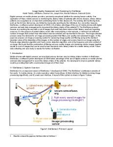
where 𝑤 = {𝑤𝑘,𝑙 | 𝑘 = −𝐾, . . . , 𝐾, 𝑙 = −𝐿, . . . , 𝐿} is a 2dimensional symmetric Gaussian weighting function and K and L are the normalized window sizes. The literature [15] shows that when calculating the local mean and variance, the performance of the algorithm is relatively stable with the change of window scale. However, when the window scale becomes very large, the performance of the algorithm will begin to decrease because the calculated mean and variance are no longer local information. 2.2. Visual Saliency. In the method proposed by Le Kang, the average value of all local quality scores for the test image is taken as the quality value for the entire image. However, such methods do not take into account human visual perception of the image, because the content of the local image block and its position in the entire image will affect the viewer’s visual perception. For example, people are less sensitive to distortion in flat areas of an image (such as blue sky) than in complex textured areas (such as edges). Each block in the image has a different effect on human-perceived image quality. We therefore use the saliency of image blocks in the following study as a weight to represent the degree of human visual perception. Figure 2 shows how to predict a saliency map.
3. Method 3.1. Input. Previous NR-IQA methods based on deep learning, such as [16, 18], consider only the information of grayscale images and ignore the distortion information contained in the color components of the image. Yet, as can be seen in Figure 3, distortion has the most significant effect on the hue component. Therefore, we use HSV as the color space and use the image hue component and grayscale information
Security and Communication Networks
(a)
3
(b)
Figure 2: Schematic detection results: (a) original image and (b) saliency map.
(a)
(b)
(c)
(d)
(e)
(f)
Figure 3: The representation of an image in the HSV color space. The first column contains the three components of the reference image in the HSV color space. The second column is the three components of the JPEG2000 distorted image in the HSV color space. (a) and (b) represent a hue component; (c) and (d) represent a saturation component; (e) and (f) represent a value component.
4
Security and Communication Networks
64
64 gray image block output
64
64 hue image block 96 feature maps
96 feature maps
convolutional layer
pooling layer
256 feature 128 feature 128 feature maps maps maps
Input Inception convolutional pooling module layer layer
192
384
fully connected concatenate layer layer
fully connected layer
Figure 4: CNN model architecture.
as the input for the CNN model to extract features related to image distortion. 3.2. CNN. In this section, we will introduce the proposed CNN model in detail. Figure 4 shows the network structure of the model. It consists of two parts. Apart from the different inputs, the other structures, including the number and size of the convolution kernels, are the same. One of the inputs is the gray scale image block and the other input is the hue image block. The size of the block is 64 × 64. For the network, the first layer is a convolutional layer with 96 convolutional kernels with size of 5 × 5 and stride of 2 pixels for each. It produces 96 feature maps with size of 30 × 30 for each. A max pooling layer follows the convolutional layer to reduce each feature map to size of 15 × 15. After the pooling layer, there is an inception module that produces 256 feature maps with size of 15 × 15 for each. The next layer is a convolutional layer with 128 convolutional kernels with size of 3 × 3 and a padding of 1 pixels. It produces 128 feature maps with size of 15 × 15 for each. Following the convolutional layer is a max pooling layer that samples feature maps to a size of 7 × 7. The sixth layer is a fully connected layer of 192 nodes. The next layer is a concatenate layer that connects two feature vectors with dimension of 192 for each layer. It has two components. The last layer is also a fully connected layer that gives the quality score of the image block. Except for the last fully connected layer, each layer is followed by a ReLUs (Rectified Linear Units) activation layer.
In addition, to prevent overfitting when training the CNN model, we apply dropout regularization with a ratio of 0.5 before the last fully connected layer. Because image quality assessment is a quantitative problem, the CNN needs continuous variable prediction. Thus, the Euclidean distance loss function is chosen as the learning loss function: E=
1 𝑁 2 ∑ 𝑦̂ − 𝑦𝑛 2 2𝑁 𝑛=1 𝑛
(4)
where 𝑦̂𝑛 is the image block quality score predicted by CNN, 𝑦𝑛 is the image block quality score, and 𝑁 is the number of blocks. 3.3. Image Quality Assessment. Through the proposed CNN model, the local image quality evaluation can be obtained. An RGB image is given, converted into a grayscale image and a hue image in the HSV color space, and then the grayscale and hue images are sampled separately. The sampled image block is then subjected to a preprocessing operation, i.e., the local contrast normalization described in (3). Figure 5 is a preprocessed gray image. Similarly, the hue image is subjected to the same sampling operation and preprocessing to obtain a corresponding hue image block. Finally, the prepared gray image block and the hue image block are inputted in pairs into the CNN model, and a series of convolution and pooling processes are performed to output the image block quality value, i.e., the local image quality evaluation.
Security and Communication Networks
5 assessment in Section 3.3, we propose a simple CNN model for evaluating the quality of denoised images, as shown in Figure 7. First, we perform a local normalization for a gray image and then sample nonoverlapping image blocks where the size is 64 × 64 pixels from normalized image. Our network consists of ten layers: 64 × 64-32 × 30 × 30-32 × 15 × 15-96 × 15 × 15-96 × 7 × 7-128 × 7 × 7-128 × 3 × 3-800-800-1. We apply a dropout regularization with a ratio of 0.5 after the second fully connected layers. Finally, we obtain average scores of all of the image blocks to represent the entire image quality score.
Figure 5: Preprocessed grayscale image blocks.
For a test image G, we obtain the corresponding saliency map S through the saliency detection model. In order to obtain the image block weight corresponding to the CNN model, we adopt a nonoverlapping sampling strategy for the saliency map S. The weight of the image block is expressed as 𝐻
c𝑘 = ∑
𝐻
∑ 𝑝𝑠,𝑘 (𝑖, 𝑗)
(5)
𝑚=−𝐻 𝑛=−𝐻
w𝑘 =
𝑐𝑘 𝑙 ∑𝑙=1 𝑐𝑘
(6)
For test image 𝐺 = [𝑃𝑔,1 , 𝑃𝑔,2 , . . . , 𝑃𝑔,𝑙 ] and saliency map 𝑆 = [𝑃𝑠,1 , 𝑃𝑠,2 , . . . , 𝑃𝑠,𝑙 ], 𝑙 is the number of blocks. There is a one-toone correspondence between 𝑃𝑔 and 𝑃𝑠 . 𝑝𝑠,𝑘 (𝑖, 𝑗) is the pixel value of the position (𝑖, 𝑗) in the significant image block 𝑃𝑠,𝑘 , and 𝑐𝑘 is the sum of the coefficients of the image block 𝑃𝑠,𝑘 . Finally, we calculate the global quality score of test image G: 𝑙
Q = ∑ 𝑤𝑘 𝑞𝑘
(7)
𝑘=1
The algorithm structure is shown in Figure 6.
3.4.2. Image Denoising Algorithm. The ROF model is one of the most effective methods for image denoising. It aims to model the problem of image denoising as a minimization of the energy function to make the image smooth while the edge can be maintained well. Generally, the total variation value of the noisy image is larger than the clear image. The effect of noise removal can be achieved by solving the minimization function of the total variance. Therefore, the ROF model for image denoising is as follows: 𝜇 2 argmin { 𝑢 − 𝑓2 + ‖𝑢‖𝑇𝑉} 2
(8)
where 𝑓 is the noise image and 𝑢 is the denoising image. The first term of the above formula is the fidelity term, so that the denoised image 𝑢 keeps as much of the information in the noise image 𝑓 as possible. The second item is the TV regular term, which allows the model to effectively preserve edges while denoising. 𝜇 > 0 is a regularization parameter. The larger 𝜇 is, the smoother the denoising image will be, resulting in blurred image. The smaller 𝜇 is, the worse the denoising effect is. Therefore, choosing a suitable 𝜇 has a great effect on the results of the denoising. There are two cases of total variance. In this section, we only consider the isotropic ROF denoising problem: 2 𝜇 2 2 √ min { (∇𝑥 𝑢) + (∇𝑦 𝑢) + 𝑢 − 𝑓2 } 2 1
(9)
Split Bregman method [22] is used to solve formula (9); assuming dx ≈ ∇x u and dy ≈ ∇y u, the image denoising problem is as follows:
3.4. Image Denoising. Nowadays, many algorithms [19–21] have achieved very good denoising effects. For example, Rudin et al. [21] proposed a classic total variation (TV) denoising algorithm in 1992, namely, the ROF model. However, an iterative denoising algorithm is always computationally intensive since it requires multiple rounds of image quality assessment to find the best parameters. To solve this problem, we propose a parameter selection framework which reduces the number of iterations of the algorithm while finding the optimal parameters, in order to save execution time.
Using Bregman iterative algorithm to solve (10), the isotropic ROF algorithm is as shown in Algorithm 1. G denotes solving the linear equations with Gauss-Seidel iteration. We focus on the influence of parameter selection on the performance of the total variation denoising algorithm.
3.4.1. No-Reference Image Quality Assessment. The assessment method for image quality will be applied to an image processing algorithm to achieve optimal parameter selection. Based on the success of the CNN model for image quality
3.4.3. The Framework of Parameter Selection. In order to study the effect of parameter selection based on image quality on denoising results, we denoise the Park image [23] with 25 different values of parameter 𝜇. The values are uniformly
𝜇 2 𝜆 2 min (𝑑𝑥 , 𝑑𝑦 )2 + 𝑢 − 𝑓2 + 𝑑𝑥 − ∇𝑥 𝑢 − 𝑏𝑥 2 2 2 𝜆 2 + 𝑑𝑦 − ∇𝑦 𝑢 − 𝑏𝑦 2 2
(10)
6
Security and Communication Networks
putput weight Test Image
Saliency map
conv
max pooling
conv
incption
max pooling
fc
Gray Image concat CNN-putput conv
max pooling
conv
incption
max pooling
fc
Hue Image
64
64
Input
96 feature maps
96 feature maps
256 feature maps
128 feature maps
128 feature maps
192
Figure 6: Algorithm architecture.
64
64 800 32 feature maps
32 feature maps
96 feature maps
800
96 128 128 feature feature feature maps maps maps
Figure 7: CNN model architecture.
sampled from 1 to 49. Figure 8(a) shows the variation of the denoised image quality in the iterative process for different parameter values. Figure 8(b) is the result of the denoised image obtained using the SSIM and CNN Q methods to evaluate different parameters. Their predicted image quality
trends are the same. It is obvious that the best denoising effect is obtained when parameter 𝜇 is 13. However, image quality assessment is performed after the completion of the whole processing of iterative convergence when the range of parameter is large. Therefore, choosing an
Security and Communication Networks
7
0.5
CNN Q
0.4 0.3 0.2 0.1 0
0
50
100
150
Iterative number mu=1 mu=13 mu=49 (a)
0.3
0.7
0.2
0.6
0.1
SSIM
CNN Q
0.8
0.5 10
20
mu
30
40
0 50
SSIM CNN Q (b)
Figure 8: (a) Iterative process of different parameter values; (b) using SSIM and CNN Q to evaluate the denoising image quality of different parameter values.
Initialize: 𝑢0 = 𝑓, 𝑑𝑥0 = 𝑑𝑦0 = 𝑏𝑥0 = 𝑏𝑦0 = 0 1: while ‖𝑢𝑘 − 𝑢𝑘−1 ‖2 > 𝑡𝑜𝑙 do 2: u𝑘+1 = 𝐺 (𝑢𝑘 ) max (𝑠𝑘 − 1/𝜆, 0) (∇𝑥 𝑢𝑘 + 𝑏𝑥𝑘 ) 3: 𝑑𝑥𝑘=1 = 𝑠𝑘 𝑘 − 1/𝜆, 0) (∇𝑦 𝑢𝑘 + 𝑏𝑦𝑘 ) max (𝑠 4: 𝑑𝑦𝑘=1 = 𝑠𝑘 5: 𝑏𝑥𝑘+1 = 𝑑𝑥𝑘 + (∇𝑥 𝑢𝑘+1 − 𝑑𝑥𝑘+1 ) 6: 𝑏𝑦𝑘+1 = 𝑑𝑦𝑘 + (∇𝑦 𝑢𝑘+1 − 𝑑𝑦𝑘+1 ) 7: end while Algorithm 1
optimum parameter in a certain range requires a very large number of iterations. Therefore, we use the changes in iteratively generated denoising image quality as a basis for determining if
if max(𝐷𝑚 , 𝐷𝑚−1 , . . . , 𝐷𝑚−𝑙 ) < 𝑇𝑞 then Converge else Continue iterating end if Algorithm 2
the iterative algorithm converges. Assuming that Dm = Q(m+1)−Q(m), Q(m) represents the quality score of the denoised image produced by the m-th iteration, and the algorithm convergence is presented in Algorithm 2. “𝑙” denotes the iterative length of the change of image quality that needs to be taken into account to ensure that the algorithm converges and produces a permissible change in image quality. The larger the “𝑙” value is, the smaller the “Tq” value becomes, indicating that the convergence condition of the algorithm is stricter.
8
Security and Communication Networks
Parameter mu={mu1 , mu2 , . . . , muk }
Start iteration
j=0 j-th iteration
j=j+1
Get q(j)
q(j)