ABSTRACT. We investigate the applicability of modified B-spline functions in digital image resampling tasks. We con- sider a modification that is based on the ...
DIGITAL IMAGE RESAMPLING BY MODIFIED B-SPLINE FUNCTIONS Atanas Gotchev1, Jussi Vesma2, Tapio Saramäki3, Karen Egiazarian3 1Tampere
Int. Center for Signal Processing, 2Telecommunications Lab, 3Signal Processing Lab Tampere University of Technology, P. O. Box 553, FIN-72101 Tampere, FINLAND, [agotchev,Jussi.Vesma,ts,karen]@cs.tut.fi ABSTRACT
We investigate the applicability of modified B-spline functions in digital image resampling tasks. We consider a modification that is based on the use of a linear combination of shifted B-splines of different degrees. By optimizing the weighting coefficients, we get interpolating functions with improved frequency responses – flatter characteristics in the passband and a higher attenuation of unwanted images of the original baseband. We realize a computationally efficient procedure, based on the use of a modified Farrow structure. In our experiments, the modified B-spline decimators and interpolators have shown a better performance and a better visual quality than their classical B-splines counterparts. 1. INTRODUCTION Image interpolation and resampling are essential tasks in many image-processing applications such as biomedical imaging, digital photography, multimedia, etc. Both tasks result in a change of the sampling rate. This change generates some artificial effects known as ringing, aliasing, imaging, blocking, and blurring [1]. Therefore, the research efforts have been concentrated on finding the most appropriate interpolating or resampling functions with an acceptable computational complexity for minimizing the above effects. Most often image interpolation is considered as fitting a continuous-time signal model with discrete data and then resampling this signal by a finer sampling step. This approach demands some assumptions on the functional space that the functions belong to. If the band-limited case is considered then the sinc (sin(x)/x) interpolator is used. Unfortunately, the sinc function decays very slowly and its approximation produces ringing and imaging artifacts. Furthermore, the most important information in images is usually carried out by the edges, which cannot be modeled as band-limited functions. An alternative assumption is that the continuous model belongs to some polynomial spline space. This gives some facilitation, especially if the splines are represented in terms of B-spline basic functions [2]. The most attractive properties of B-splines are their compact support, sufficient regularity, smooth behavior, and easy implementation [1], [2]. The spline bases, as the ones described in [1], are separable so that the 2-D resampling problem can be reduced to 1-D case.
As far as image reduction is concerned, the minimization of the aliasing effects requires prefiltering. The prefilter depends exactly on the chosen reconstruction (interpolation) method. In the case of band-limited functions, an ideal low-pass prefilter (sinc convolver) is applied. The combination of an ideal low-pass prefilter and sinc interpolation ensures the least squared reconstruction error. For the case of spline interpolation (assumption for non band-limited functions) the optimal solution leads to prefilters different from the sinc convolver [3], [4]. Despite their good properties, B-spline interpolators do not provide sufficiently precise approximation in many applications. This makes it necessary to develop new spline bases for signal representation. A new parametric class of modified B-splines has been introduced in [5]. In general, the proposed spline functions have been represented by a linear combination of weighted and shifted classic B-splines of different degrees. Later, with the similar objectives – improving the approximation properties of B-spline functions - Blu et al. [6] introduced the so-called Moms (maximum order, minimum support) functions which are generated by a linear combination of a B-spline of a certain order and its derivatives. In this paper, the modified B-splines introduced in [5] are studied for their applicability for effective image resampling. A number of digitalized images have been resampled by the prefilters obtained in the consideration that modified B-spline interpolators should be used for the reconstruction. An optimization procedure is used for finding the best weighting parameters. Experimental results show that the proposed modified B-spline interpolating functions with appropriately optimized weighting coefficients perform better than the classical Bspline interpolators and the theoretically optimized Moms. 2. MODIFIED B-SPLINE RESAMPLING FUNCTIONS 2.1. Interpolators 2.1.1. Generalized interpolation model The generalized 1-D interpolation model is considered as follows [1]:
s ( x) =
∑ c(k )ϕ ( x − k ) ,
(1)
k∈Z
where ϕ (x) is the generating (interpolation) function, the c (k ) ’s are the convolution coefficients, and s (x) is a continuous-time function that coincides at the integers with the signal data s (k). This interpolation condition determines one additional step in comparison to the ordinary interpolation. One needs to obtain the model coefficients c (k ) . Imposing s (l ) = ∑ c(k )ϕ (l − k ) we ark∈Z
rive at the interpolation scheme shown by Fig. 1. Here ϕ (k ) −1 is the convolution inverse. s(k)
c(k)
s(x)
ϕ(k)-1
ϕ(x)
modeling
interpolating
Figure 1. Generalized 1-D interpolation model. 2.1.2. Classical B-splines as interpolators For the classical B-spline case, ϕ ( x) = β n ( x ) is a central B-spline of degree n:
β n ( x) = β 0 ( x) ∗ β n −1 ( x )
(2)
1, x ∈ [− 1 / 2, 1 / 2) β 0 ( x) = . otherwise 0,
(3)
They are in the function class Cn-1, i.e., they are the most regular functions of degree n with a support of n+1 and an approximation order L=n+1 [2]. When sampled at the integers, the B-splines are symmetrical finitelength sequences. Hence, the first step in the 1-D interpolation model becomes pure IIR filtering. It can be realized efficiently by decomposing in first order filters and applying successively in forward and backward directions [6], or by an efficient FIR approximation [5]. 2.1.3. Modified B-spline case We consider a modification of the interpolation function ϕ (x) of the following form: N
ϕ ( x) = ∑ a n ( x ) ,
(4)
n =0
A similar modification, referred as o-moms, has been introduced in [6]: N
ϕ ( x) = ∑ γ k k =0
dk N β ( x) . dx k
Again, the highest degree N must be an odd integer, in order to get a well-optimized solution for γk’s [6]. 2.1.4. Comparison between classical and modified Bsplines Modified and classical B-splines, as well as the Moms can be indexed by their degree n. They have the same approximation order L=n+1 and the same support n+1 [1]. Moreover, the classical B-splines are the most regular functions of degree n. When applying for interpolation, the functions of the form of Eq. (4) and (5) offer more degrees of freedom and are very susceptible to optimization. Through adjusting the parameters γ nm , one can choose different optimization strategies. In our experiments we have been optimizing them in such a way, that the images of a certain fraction of the interval [0, Fs / 2] with Fs being the sampling rate, are attenuated as well as possible [5]. Our hypothesis has been that by this approach we do safe the smoothing properties of the splines of degree n, giving them the freedom to preserve contours by improving their frequency behavior in these areas. The o-moms themselves have been constructed in the assumption that they have to minimize the asymptotic approximation error, when the sampling step tends to zero. So, they are well applicable for the images with a very low-frequency content. They perform better than classical B-spline interpolators in the overall frequency range, but not so well as the modified B-splines around the image edges. 2.2. Decimators (prefilters) Suppose that the initial 1-D continuous-time function s has been sampled and we want to reconstruct it by interpolation model (1). Then Eq. (1) can be rewritten in the matrix form as follows: ~ (7) s = Ac , where A denotes a linear transformation in the form of an infinite matrix, taking a coefficients sequence into the reconstructed function ~ s ( x ) . The least-squared solution to the coefficients c is given by [3]: c = (A * A) −1 A * s .
where a n ( x) =
MN
∑γ
nm
β n ( x − m)
(5)
m=−M N
assuming n and N are odd integers and m depends on the support of the B-spline of the highest degree. It is required that ϕ (x) is symmetrical. Therefore, γ mn = γ −mn .
(6)
(8)
Here A* is the adjoint operator to A. In fact, this solution is a projection of the function s onto the polynomial space generated by ϕ ( x − k ) (here the sampling rate is supposed to be equal to unity) and the linear operator ( A * A) −1 A * represents the dual basis ϕ~ ( x − k ) [4]. For the case of resampling, when the initial function (image row or column) is discrete, Eq. (8) will minimize the l2
norm [3]. It can be considered to be optimal with respect to the fixed interpolator filter. The overall scheme of resizing-reconstruction by an arbitrary decimation/interpolation factor using (modified) B-splines is shown in Fig. 2. c(k)
ϕ~( x / ∆ − k ) orthogonal projection
0
−20
s(x)
ϕ(x)
interpolation
Figure 2. Decimation-interpolation task
Magnitude in dB
s(k)
B-spline values at arbitrary points. The same operation is requisite in the interpolation step of Fig. 2.
−40
−60
−80
−100 0
0.5
1
1.5
2
2.5
3
3.5
4
Frequency in F
s
2.3. Optimization strategy The main idea of using a linear combination of Bsplines is that we can improve the performance of the interpolator without increasing the complexity. When combining the cubic spline and linear splines, we preserve the support (and hence the complexity) together with the smooth behavior of the 3rd degree B-spline and try to assure more possibilities for adequate representation of edge areas. Hence our optimization task can be defined as follows: • Assume that the most important signal components are in the frequency range f ≤ α Fs 2 , with α < 1 Fs being the sampling frequency. • Let δ s be the maximum amplitude deviation of the interpolation filter from zero in the image frequencies, i.e. in the frequency range kFs (1 − α ) ≤ f ≤ kFs (1 + α ) for k=1,2,3… . • Let δ p be the maximum amplitude deviation
•
•
from unity in the passband, i.e. in the frequency range 0 ≤ f ≤ α f s 2 . In order to fulfill the partition of unity condition [1], which implies that the amplitude response is unity at zero frequency, it is required γ 10 = −2γ 11 . Given α and a weighting parameter w, find γ 10 to minimize max(δ p w , δ s ) .
An example is given in Fig. 3. Here, α =0.6 and the optimized coefficients are γ10=-0.0848 and γ11=0.0424. They assure an attenuation of images of 43.4 dB. 3. EFFICIENT REALIZATIONS The orthogonal projection given by Eq. (8) can be realized efficiently by the finite differences method developed in [8]. The algorithm is based on the evidence that the orthogonal projection in Fig. 2 is equivalent of a higher order B-spline interpolation. Then the most computationally expensive step is the calculation of the
Figure 3. Frequency responses of the modified 3rd +1st degree (solid line), 3rd degree (dashed line), o-moms (dot-dashed line) B-spline interpolators. Since the B-splines and their modifications can be considered as piece-wise polynomial-based functions, they can be very efficiently realized using a modified Farrow structure [7]. We give here an example for the case of the modification of B-splines of 3rd and 1st degrees, although other modifications are also possible. The generating function can be written as follows:
ϕ ( x) = β 3 ( x ) + γ 10 β 1 ( x ) + γ 11 β 1 ( x − 1) + γ 11 β 1 ( x + 1) (9) Replacing the continuous-time variable x by a fractional variable µ=x-m and developing Eq. (1) in a polynomial form with respect to µ, we can express s(µ) in the following matrix form: s(µ ) =
*F ,
1 6
(10)
where
[
= µ3
µ2
−1 3 G= − 3 − 6γ 11 1 + 6γ 11 c = [c m − 2
c m −1
]
µ 1 1; 3 −6
−3 3
− 6γ 10 + 6γ 11 4 + 6γ 10
3 + 6γ 10 − 6γ 11 1 + 6γ 11
cm
c m +1 ] .
; − 6γ 11 0 1 0
T
Eq. (10) represents a filter structure of four FIR filters having fixed coefficients. The only value, which has to be loaded to the interpolator, is the current fractional interval µ. The modified Farrow structure is shown in Fig. 4 where Gj(z) represents the jth row of the matrix G. 4. EXPERIMENTS In our experiments we have performed successful image decimation and reconstruction, using the B-spline interpolating functions of different degrees, the o-moms, and
the recently developed modified B-spline functions. We have compared the SNRs between the initial and reconstructed images. The modified B-spline functions with optimized weight parameters have shown a better performance (higher SNRs) and a better visual quality (better contour preservation). c(k)
G3(z)
G2(z)
G1(z)
G0(z)
s(x)
µ Figure 4. Modified Farrow structure. Some results are summarized in Table 1. They represent three successive resizing operations with factors 0.5957, 0.6074, and 0.6504 (Baboon3 and Barbara3), and five successive resizing operations with factors 0.5957, 0.6074, 0.6504, 0.6855, and 0.6072 (Barbara5). A detail of Barbara3 experiment is shown in Fig.5. 5. CONCLUSIONS We have chosen an optimization procedure in the frequency domain, which describes the joint action of 3rd and 1st degree B-splines as sufficient suppression of imaging frequencies, together with the sharp transition between passband and stopband regions. This optimization technique allows us to preserve the details, better modeled with first-degree basic functions, taking advantage also of the smoother 3rd degree B-spline. Total computational complexity is practically equal to the classical B-spline interpolator’s complexity. We have proposed a modified Farrow structure that lowers the complexity and is very appropriate for real-time applications.
[5] K. Egiazarian, T. Saramäki, H. Chugurian, and J. Astola, “Modified B-spline interpolators and filters: synthesis ans efficient implementation”, In Proc. IEEE Int Conf. ASSP, Atlanta, USA, May 1996, pp. 17431746. [6] T. Blu, P. Thevenaz, and M. Unser, “Minimum Support Interpolators with Optimum Approximation Properties”, in Proc. IEEE Int. Conf. Image Processing, Chicago, USA, October 1998, pp. WA06.10. [7] J. Vesma and T. Saramäki, “Interpolation filters with arbitrary frequency response for all-digital receivers”, in Proc. Int. Symposium Circuits and Systems, Atlanta, USA, May 1996, pp.568-571. [8] A. Munos, T. Blu, and M. Unser, “Efficient Image Resizing Using Finite Differences”, in Proc. Int. Conf. Image Processing, Kobe, Japan, October 1999, pp. 662666. [9] C. Farrow, “A continuous variable digital delay element”, in Proc. Int. Symposium Circuits and Systems, Espoo, Finland, June 1988, pp.2641-2645. SNR, [dB] Synthesizing function
β3 β 31, o-moms β 31, α=0.8
γ10 0 -0.0476 -0.1204
Baboon3 24,51 24,60 24,76
Barbara3 25,76 25,87 26,13
Barbara5 25,65 25,79 26,08
Table 1. Experimental results for successive decimations and interpolations.
6. ACNOWLEGEMENTS Authors wish to thank the Median Free Group International for helpful suggestions and nice working atmosphere during the preparation of this work. 7. REFERENCES [1] P. Thevenaz, T. Blu, and M. Unser, “Image Interpolation and Resampling”, in Handbook of Medical Image Processing, in press. [2] I. Schoenberg, “Cardinal interpolation and spline functions”, J. of Approximation theory, vol. 2, pp. 167206, 1969. [3] R. Hummel, “Sampling for spline reconstruction”, SIAM J. Appl. Math., vol. 3, No. 2, pp. 278-288, 1983. [4] M. Unser, A. Aldroubi, and M. Eden, “Polynomial Spline Signal Approximations: Filter Design and Asymptotic Equivalence with Shannon’s Sampling Theorem”, IEEE Trans. Information Theory, vol. 38, No. 1, pp- 95-103, 1992.
Figure 5. A detail of Barbara3 experiment after three successive decimations and interpolations. From left to right and from top to bottom: Initial image; restored image by β 3 interpolator; restored image by o-moms interpolator, restored image by the modified β 31-spline interpolator.