[10], conducted a comprehensive performance evaluation among several global/spatial color descriptors for CBIR and reported that correlogram achieves the ...
Directional Spatial Color Descriptor in a Perceptual Model: Proximity Grids Serkan Kiranyaz, Murat Birinci and Moncef Gabbouj1 Tampere University of Technology, Tampere, Finland {serkan.kiranyaz, murat.birinci, moncef.gabbouj}@tut.fi Abstract Most of the color features widely used in content-based image retrieval (CBIR) present severe limitations and drawbacks due to their inefficiency of modeling human visual system on color perception. Accordingly, they are not capable of characterizing both spatial and global properties of the color composition in visual scenery. In this paper, we present a perceptual color feature, which describes the global properties of the prominent colors along with a directional spatial descriptor, called as Proximity Grids. In color domain the dominant colors are extracted along with their global properties and quad-tree decomposition partitions the image so as to characterize the spatial color distribution (SCD). This approach is in accordance with the well-known Gestalt law, i.e. utilizing a top-down approach in order to model (see) the whole color composition before its parts and in this way we can avoid the problems of pixelbased approaches. The proximity grids, which cumulate the spatial co-occurrence of colors in a 2D grid, can successfully model the SCD of the prominent colors with respect to inter-color proximities and directions. Fusing both global and spatial properties forms the final descriptor, which is neither biased nor become noisy from the presence of such color elements, the socalled outliers that are not visible for humans in both spatial and color domains. Finally a penalty-trio model cumulates the differences among the color properties in a similarity distance computation during retrieval. Comparative evaluations against well-known global and spatial descriptors demonstrate the superiority of the proposed descriptor.
1. Introduction There is a wealth of research done and still going on in developing content-based multimedia indexing and retrieval systems such as MUVIS [9], QBIC [7], PicHunter [4], Photobook [16], VisualSEEk [19], Virage [22], VideoQ [3], etc. In such frameworks, database primitives are mapped into some high dimensional feature domain, which may consist of several types of descriptors. Among them careful selection of some sets to be used for a particular application may capture the semantics of the database items in a content-based multimedia retrieval (CBMR) system. In this paper we shall restrict the focus on CBIR domain, which employ only color as the descriptor for image retrieval. Recently the study of human color perception and similarity measurement within the color domain become crucial and there is a wealth of research performed in this field such as [2], [12] and [13]. One perceptual fact from these works is that human eye cannot perceive a large number of colors at the same time, nor able to distinguish similar (close) colors well. Based on this, they show that at the coarsest level of judgment, HVS primarily uses dominant colors (i.e. the few colors prominent in the scenery) to judge similarity. Henceforth, the two rules are particularly related for modeling the similarity metrics of
1
the human’s color perception. The first one indicates that the two color patterns that have similar dominant colors (DCs) are perceived as similar. The second rule states that two multicolored patterns are perceived as similar if they possess the same (dominant) color distributions regardless of their content, directionality, placement or repetitions of a structural element. Furthermore, it is obvious that humans can neither see individual pixels, nor perceive even a tiny fracture of such a massive amount of color levels, which are present in nowadays digital imaging technology and thus it is crucial to perform certain steps in order to extract the true “perceivable” elements (the true DCs and their global distributions). Under the light of these perceptual facts, in this paper, we present a systematic approach to extract such a perceptual (color) descriptor and then propose an efficient similarity metric to achieve the highest discrimination power possible for the color-based retrieval in general-purpose image databases. We adopt a top-down approach both in DC extraction and modeling their global spatial distribution. This approach is in fact phased from the well-known Gestalt rule of perception: “Humans see the whole before its parts”, therefore, the method strives to extract what is the (next) global element both in color and spatial domain, which are nothing but the DCs and their spatial distribution within the image. In order to achieve such a (compact) spatial representation within an image, starting from the entire image, quad-tree decomposition is applied to the current (parent) block only if it cannot host the majority of a particular DC, otherwise it is kept intact (non-decomposed) representing a single, homogeneous DC presence in it. So this approach tries to capture the “whole” before going through “its parts” and whenever the whole body can be perceived with a single DC, it is kept “as is”. Hence the outliers can be suppressed from the spatial distribution and furthermore, the resultant (block-wise) partitioned scheme can be efficiently used for a global modeling and due directional description of the spatial distribution via inter-proximity statistics of the DCs using Proximity Grids. Finally a penalty-trio model uses both global and spatial color properties and performs an efficient similarity distance computation.
2. Related Work Swain and Ballard [21] proposed the first color histogram, which is quite simple to implement and gives reasonable results especially in small to medium size databases. Thus several other histogram-based approaches emerged, such as [4], [6], [7], [9], [16], [18], etc. The primary feature of such histogram-based color descriptors (be it in RGB, CIE-Lab, CIE-Luv, or HSV) is that they cluster the pixels into fixed color bins, which are quantizing the entire color space using a pre-defined color palette. Yet their performance is still quite
1 This work was supported by the Academy of Finland, project No. 213462 (Finnish Centre of Excellence Program (2006 - 2011) The research leading to this work was partially supported by the COST 292 Action on Semantic Multimodal Analysis of Digital Media
limited and usually degrades drastically in large databases due to several reasons. First and the foremost, they apply staticquantization where the color palette boundaries are determined empirically or via some heuristics –yet nothing based on human color perception rules. No matter how the quantization level (number of bins) is set, pixels with such similar colors but either side of the quantization boundary, which separates two consecutive bins will be clustered into different bins and this is an inevitable source of error in all histogram-based methods. The color quadratic distance [7] proposed in the context of QBIC system provides a solution to this problem by fusing the color bin distances into the total similarity metric. This formulation allows the comparison of different histogram bins with some inter-similarity between them; however it underestimates distances because it tends to accentuate the color similarity [20]. Furthermore, Po and Wong in a recent study [17] show that it does not match the human color perception well enough and may result incorrect ranks between regions with similar salient color distributions. Hence it gives even worse results than the naïve L p metrics on some particular cases. In order to solve the problems of the color histograms applying such a static quantization scheme, various DC descriptors [1], [5], [11], [13], etc., using dynamic quantization with respect to image color content are developed. DCs, if extracted properly according to aforementioned color perception rules, can indeed represent the prominent colors in any image. They have a global representation, which is compact and accurate and they are also computationally efficient since only few colors that are usually present in a natural image and perceivable by a naked human eye are described. Although the true DCs, which are extracted via such perceptually oriented scheme with the proper metric can address the aforementioned problems of color histograms, global color properties (DCs and their coverage areas) alone are not enough for characterizing and describing the real color composition of an image since they all lack the crucial information of spatial relationship among the colors. In other words, describing “what” and “how much” color is used will not be sufficient without specifying “where” and “how” the (perceivable) color components (DCs) are distributed within the visual scenery. Especially in large image databases, this is the main source of erroneous retrievals, which makes “accidental” matches between images with “similar” global color properties; however different in the color distribution. There are several approaches to address this problem such as [6], [20], [14], etc., all of which apply fixed partitioning and use the block positions alone for matching. Therefore, such methods become strictly domain dependant solutions since they cannot provide any reliable description for SCD in general. One of the most promising approach among all SCD descriptors is the color correlogram [8], which is a table where the kth entry for the color histogram bin pair (i, j) specifies the probability of finding a pixel of color-bin j at a distance k within a maximum range d, from a pixel of color-bin i in an image I with dimensions W x H. Accordingly, Ma and Zhang [10], conducted a comprehensive performance evaluation among several global/spatial color descriptors for CBIR and reported that correlogram achieves the best retrieval performance among the others, such as color histograms, Color Coherence Vector (CCV) [15], color moments, etc. However, the computation complexity is a critical factor for the feasibility of correlogram. The naïve algorithm to compute correlogram takes O (W .H .d 2 ) , which is a massive
computation.
The
fast algorithm can reduce this
to
O(5.W .H .d ) ; however requiring O(16.W .H .d .m) memory space (in bytes) to store them. Another computational issue is the storage of the feature vector. Since the feature vector size of correlogram (in bytes) is O (16 m 2 d ) , a simplified version, the so-called autocorrelogram, which only captures the spatial correlation between the same colors and thus reduces the feature vector size to O (16 md ) bytes, is also proposed in [8]. Nowadays digital image technology offers several mega-pixel (Mpel) image resolutions. For a conservative assumption, consider a small size database with only 1000 images each of which in only 1 Mpel resolution. So without loss of generality, assume W,H~1000 respectively. In such image dimensions, any d setting less than 100 pixels would be too small for characterizing the true SCD of the image –probably describing only a thin layer of adjacent colors (i.e. colors that can be found within a small range). Assume the lowest range setting: d=100 even with such “minimal” settings, the naïve algorithm will require ~ O (1010 ) computations. Even with the fast computers, an infeasible time is required to index even a small database. The only alternative is to use the fast algorithm. With the typical quantization for RGB color histogram (i.e. 8x8x8=512 bins), the fast algorithm will speed up the process around 25 times; however, it will also require a massive memory, (> 400Gb per image) and this time neither decimation, nor drastic reduction on the range will make it feasible. Furthermore, its massive storage requirement is another serious bottleneck of the correlogram. Note that for the minimal range (d=100) and typical quantization settings (i.e. 8x8x8 RGB partitions), the amount of required space for the feature vector storage of a single image is above 400Mb. To make it work, the range value has to be reduced drastically along with using a much coarser quantization (4x4x4 bins or less). Unfortunately with such settings, recall the problems of coarse quantization of color histograms and such a diminished range setting. The only alternative is computing autocorrelogram instead of correlogram, which is eventually recommended and used in [8]; however without characterizing spatial distribution of distinct colors with respect to each other, the true SCD cannot be accurately described. Apart from such severe feasibility problems, correlogram has several limitations and drawbacks. The first and the foremost is its pixel-based structure, which characterizes the color proximities in pixel level. Such a high-resolution description not only makes it too complicated and infeasible to perform, it also becomes meaningless with respect to HVS color perception rules simply because individual pixels do not mean much for human eye. As an example, consider a correlogram description such as “the probability of finding a red pixel in a 43 pixel proximity of a blue pixel is 0.25” and so what difference does it make to have this probability in 44 or 42 pixels proximity for human perception? Furthermore, since correlogram is a pixel level descriptor working over RGB color histogram, the outliers, both in color and spatial domains will cause the aforementioned feasibility problems on computational (memory and speed) cost and storage, which makes correlogram inapplicable in many cases or significantly degraded and limited so as to make it feasible again. Finally using the probability alone, makes the descriptor insensitive from the dominance of the color or its area (weight) in the image. This is basically due to the normalization by the amount (weight or area) of color and such an important perceptual cue is lacking in correlogram’s description. This might be a desirable property to find the similar images simply “zoomed” as in [8], and hence the color areas significantly vary but the
distance probabilities do not; however it also causes severe mismatches especially in large databases since the probability of the pair-wise color distances might be same or close independent of their area in the image and hence regardless of their dominance (be them DCs or outliers).
3. The Proposed Color Descriptor Under the light of earlier discussion, the proposed color descriptor is designed to address the drawbacks and problems of the color descriptors, particularly the correlogram. In order to achieve this, it is mainly motivated from human color perception rules and therefore, global and spatial color properties are extracted and described in a way HVS perceives them. 3.1. Formation of the Color Descriptor We adopt a DC extraction algorithm similar to one in [5] where the method is entirely designed with respect to HVS color perceptual rules and configurable with few thresholds, TS (color similarity), TA (minimum area), ε D (minimum distortion) and
max N DC (maximum number of DCs). As the first
step, the true number of DCs present in the image max (i.e. 1 ≤ N DC ≤ N DC ) are extracted in CIE-Luv color domain and back-projected to the image for further analysis involving extraction of the spatial properties (SCD) of DCs. Let
Ci represents the ith DC class (cluster) with the following members: ci is the color value (centroid), and wi is the weight (unit normalized area) Due to the DC thresholds set beforehand, wi > TA , ci − c j > TS for 1 ≤ i, j ≤ N DC . During the back-projection phase, the DC, which has the closest centroid value to a particular pixel color, will be assigned to that pixel. As a natural consequence of this process, spatial outliers can emerge. They are nothing but the isolated pixel(s), which are not populated enough to be perceivable and therefore, should be eliminated before extracting the spatial color features for characterizing the SCD of the image. Due to the perceptual approach based on the Gestalt rule, “Humans see the whole before its parts”, a top down approach such as quadtree decomposition can process the “whole” first, meaning the largest blocks possible, which can be described (and perceived) by a single DC, before going into its “parts”. Due to its topdown structure, it is not degraded from the aforementioned problems that pixel-based approaches usually do and starting from the entire image where DCs are already back-projected it extracts the largest “rectangular” blocks, which makes further analysis easier and more efficient than the arbitrary shape regions. Two parameters are used to configure the quad-tree:
TW ,
which is the minimum weight (dominance) within the
current block required from a DC not to go down for further max partition and DQT , which is the depth limit indicating the maximum amount of partition (decomposition) allowed. Note that with the proper setting of
max TW and DQT ,
QT
decomposition can be carried out to reach the pixel level; however such an extreme partitioning should instead be avoided not to deal with the aforementioned problems of pixel level analysis. Using a similar analogy
TW can
be set in
accordance with TA , i.e. TW ≅ 1 − TA . Therefore, for the
typical TA setting (between 2-5%), max QT
as TW ≥ 95% . Since D
TW can be conveniently set
determines when to stop the
partitioning abruptly, it should not be set too low not to cause inhomogeneous (mixed) blocks and on the other hand, max extensive experimental results suggest that DQT > 6 is not required even for the most complex scenes since the results are max almost identical to one with DQT = 6 . Therefore, the typical max range is 4 ≤ DQT ≤ 6 . Let
B p corresponds to pth partition of
the block B where p=0 is the entire block and 1 ≤ p ≤ 4 represents the pth quadrant of the block. The 4 quadrants can be obtained simply by applying equal partitioning to the parent block or via any other partitioning scheme, which is optimized to yield most homogenous blocks possible. For simplicity we use the former case and accordingly a generic QT algorithm, QuadTree, can be expressed as follows: QuadTree (parent, depth) ¾
Let
wmax be the weight of the DC, which has
the maximum coverage in parent block. ¾ If ( wmax
0
Let B = parent For ∀p ∈ [1,..,4] do:
¾ ¾ o ¾
> TW ) then Return.
p
QuadTree ( B , depth) Return.
The QT decomposition of a (back-projected) image I can then be initiated by calling QuadTree (I, 0) and once the process is over, each QT block carries the following data: its max depth D ≤ DQT , where the partitioning is stopped, its location in the image and the major DC, which has the highest weight in the block (i.e. wmax > TW ) and perhaps some other DCs, which are eventually some spatial outliers due to their minority. In order to remove those spatial outliers, a QT backprojection of the major DC into its host block is sufficient. The final scheme where outliers in both color and spatial domains are removed and the (major) DCs are assigned (back-projected) to their blocks can be conveniently used for further (SCD) analysis to extract spatial color features. Note that QT blocks can vary in size depending on the depth, yet even the smallest (highest depth) block is large enough to be perceivable and carry a homogenous DC. So instead of performing pixel-level analysis such as in correlogram, the uniform grid of blocks in max the highest depth ( D = DQT ) can be used for characterizing the global SCD and extracting the spatial features in an efficient way. A proximity grid represents the inter-occurrence of one DC with respect to another over a 2D (proximity) grid from which both distance and direction information can be obtained. Note that inter-color distances are crucial for characterizing the SCD of an image; however, the direction information may or may not be useful depending on the content. For example, the direction information in “17% of red is 8 units (blocks) right of blue” is important for describing a national flag picture (and hence the content) but “One black and one white horse are running together on a green field” is sufficient to describe the content without any need to know the exact directional order of black, white and green.
Let the image I have NxN blocks, each of which hosts a c single DC. 2D proximity grid, Ψc j ( x, y) , is formed by i
cumulating the co-occurrence of blocks hosting
cj
(i.e.
∀b j I (b j ) = c j ) in a certain vicinity of the blocks hosting
ci (i.e. ∀bi I (bi ) = ci ) on a 2D (proximity) grid. In other words, via fixing the block bi (hosting ci ) in the center bin of the grid (i.e. x=y=0), the particular bin, which corresponds to the relative position of block b j (hosting c j ) is incremented by one and this process is repeated for all blocks hosting c j in a certain vicinity of bi . Then the process is repeated for the next block (hosting ci ) until the entire image blocks are scanned for the color pair
ci - c j . As a result the final grid bins represent
the inter-occurrences of the hosting
color ci ,
c j blocks with respect to the ones
within
a
certain
range
L
(i.e.
∀x, y ∈[−L, L], L ≤ N − 1 ). Although L can be set as N-1 for a full-range representation, it is, however, a highly redundant setting since L ≥ N 2 cannot be fit exactly for any block without exceeding the image (block) boundaries. Therefore, L < N 2 would be a reasonable choice for L.
X
X
c
Ψci j ( x, y )
This process is illustrated on a sample image shown in Figure 1. During the raster-scan of uniform blocks, the block with white DC updates only three proximity grids (white to white, brown and blue) since those DCs can only be found within the range of ± L . For illustration purposes we kept max DQT = 5 ⇒ N = 32 and L as 4. As a result proximity grid characterizes both inter-DC proximities and the relative spatial position (inter-DC direction) between two DCs. Note that c Ψc j (0,0) = 0 for i ≠ j and Ψcci (0,0) indicates the total i
i
number of blocks hosting ci . Since this is not a SCD property –rather a local DC property showing a noisy approximation of wi (weight of ci ), it can be conveniently excluded from the feature vector and the remaining (2L +1)2 −1 grid bins are (unit) normalized by the total number of blocks, the
final
cj
Ψ ci ( x, y)
descriptor,
+1+1+1+1
ci {white} ⇒ c j {brown}
ci {white} ⇒ c j {blue}
+1+1+1 +1+1+1+1 +1+1+1+1+1+1+1+1 +1+1+1+1+1+1+1+1+1 +1+1+1+1+1+1+1+1+1 +1+1+1+1+1+1+1+1+1 +1+1+1+1+1+1+1+1+1 +1+1+1+1+1+1+1+1+1 +1+1+1+1+1
ci {white} ⇒ c j {white}
Figure 1: The process of proximity grid formation for the block (X) for L=4. c
The computation of Ψc j ( x, y) can be performed in a single i pass through image blocks. Let bi = ( xi , yi ) be the next block hosting the DC
ci . Fixing the bi in the center (i.e. Ψcc (0,0) ), j
i
all the image blocks within the range L from
bi (i.e.
∀b j = ( xi + x, yi + y ) ∈ I ∀x, y ∈ [− L, L ] ) are scanned and c
the corresponding (proximity) grid bin, Ψc j ( x, y ) , for a color i
c j in a block b j = ( xi + x, yi + y ) ∈ I is incremented by one.
where
cj
Ψ ci ( x, y) ≤ 1, ∀x, y ∈ [− L, L] . Proximity grid computation takes O( 4 N 2 L2 ) , which is independent from original image dimensions, W and H, and for a full range process, ( L = N 2) , O( N 4 ) computations is max max required. For DQT = 5 ⇒ N = 32 and N DC = 8 , as the typical
settings, it requires ~ O (10 6 ) computations, which are 10000 times less when compared to correlogram with a minimal range setting (i.e. 10% of image dimension range). In fact the real speed enhancement is much more than that since the computations in correlogram involves several additions, multiplications and worst of all, divisions (which are hundreds of times costlier than additions) for probability computations whereas proximity grid computation only requires incrimination, which is less costlier than even addition operations. The memory space requirement is in 2 O(16 N DC .L2 ) and for a full range process ( L = N 2) with the typical settings, the memory required per database image will be 256Kb, an insignificant amount compared to c correlogram. Since Ψc j ( x, y) = Ψcci (− x,− y ) (symmetric i
+1+1+1+1+1+1 +1+1+1+1+1 +1
N 2 , to form
j
with respect to origin), the storage (disc) space requirement is even lesser, O(16 N DC + 1 L2 ) ; however this is the (maximum)
2
cost of computing full-range proximity grid and therefore, it is recommended to employ the typical grid dimension range (e.g. N 8 < L < N 4 ) to reduce this cost to an acceptable level. 3.2. Similarity Distance Computation via Penalty-Trio Model In a retrieval operation in MUVIS, a particular feature of the query image, Q, is used for (dis-) similarity measurement with the same feature of a database image, I. Repeating this process for all images in the database, D, and ranking the images according to their similarity distances yield the retrieval result. The proposed color descriptors of Q and I contain both global
and spatial color properties. Let
CiQ and C Ij represent the ith
I Q Q and jth ( i ≤ N DC , j ≤ N DC ) DC classes where N DC and I are number of DCs in Q and I respectively. Along with N DC
these global properties, the proposed SCD descriptors of Q and c I contain proximity grid ( Ψc j ( x, y ) ). Henceforth for the i
similarity distance computation over the proposed color
descriptor, both global and spatial color properties are used within a penalty-trio model, which basically penalizes the following properties: • Pφ : The amount of different (mismatching) DCs •
The differences of the matching DCs in: o PG : Global color properties
PSCD: SCD properties
o
So the penalty-trio over all color properties can be expresses as,
PΣ (Q, I ) = Pφ (Q, I ) + (αPG (Q, I ) + (1 − α ) PSCD (Q, I ))
(1)
where PΣ ≤ 1 is the (unit) normalized total penalty, which corresponds to (total) color similarity distance and 0 < α < 1 is the weighting factor between global and spatial color properties. Therefore, the proposed penalty-trio model computes a complete distance measure from all color properties. Color (DC) matching is the key factor here. We form two sets: matching ( S classes from
M
C Q and C I by assigning each DC, ci ∈ Ci , in
one set, which cannot match any DC, (i.e. c i − c j > TS least
one
φ
) and mismatching ( S ) DC
φ
into
M
S .
Note
directly be expressed as, Ci ∈ S φ )
computed accordingly via one-to-one matching, Due to space limitations, we skipped the details of DC fusing operation. Afterwards, the number of DCs in both (updated) M
M
sets, S Q , S I become equal (i.e. SQM = S IM = N M ) and oneto-one matching prevails. Assume without loss of generality that ith DC class in set CiQ : {ciQ , wiQ , σ iQ } ∈ S QM matches to ith DC in set CiI : {ciI , wiI , σ iI } ∈ S IM (i.e. via sorting one set with respect to other). So the penalties for global and SCD properties can be expressed as, NM
NM
PG (Q, I ) = β ∑ wiQ − wiI + (1 − β ) i =1
that
S M + S φ = C Q + C I and using the DCs in S φ , Pφ can
∑ (w
DC sets in Q (or I), matching a single DC in I (or Q) should be first fused into a single DC and then PG and PSCD can be
c j ∈ Ci , in the other
for ∀i, j ) into S and the rest (with at
match)
in color composition of the scenery or its pre-fixed parameters (thresholds), it can result over- or under-clustering. Therefore, similar color compositions can be clustered into different number of DCs and enforcing one-to-one matching misses a certain part of matching DCs from both global and spatial similarity computation and erroneous results occur. In order to provide a solution to the problem of one-to-one matching and compute PG and PSCD while considering all the DCs matching,
N M NM
L
∑∑ ∑ PSCD (Q, I ) =
i =1 j =1 x , y = − L
c Qj
∑ (c
Q i
− ciI
i =1
)
2
Td N M
≤1
(3)
c Ij
Ψ cQ ( x, y ) − Ψ c I ( x, y ) i
(2L + 1)
i
2
≤1
total amount (weight) of DCs mismatching. In an extreme case where there are no colors matching, S M = {φ} ⇒
where 0 < β < 1 , similar to α , is the weighting factor between the two global color properties: DC weights and centroids. As a result the combination of PG and PSCD represent the amount of dissimilarity occur in the color properties and the unit normalization allows the combination in a configurable way with weights α , β , which can favor one
PΣ = Pφ = 1 makes sense since color-wise two images are
color property to another. With the combination of
nothing in common and hence entirely dissimilar. In another extreme case where all DCs are matching, so S φ = {φ } ⇒ Pφ = 0 and color (dis-)similarity will only
penalty trio models a complete similarity distance between two color compositions.
Pφ (Q, I ) =
The dissimilarity (penalty,
i
2
≤1
(2)
Pφ ) increases proportional with the
emerge from global ( PG ) and spatial ( PSCD) color properties of the (matching) DCs. Typically
Pφ contributes a certain color distance as a
natural consequence of mismatching colors between Q and I, yet the rest of the distance will occur from the cumulated difference from the properties of matching colors (due to global or spatial properties). This is, however, not straightforward to compute since one DC in Q can match one or more DCs in I (or vice versa). One solution is to apply color quadratic distance [7] to fuse DC distances into the total similarity metric; however besides its serious drawbacks mentioned earlier, this formulation can be applied only to distance calculation from global DC properties and hence cannot address how to fuse SCD distances (from proximity grid each individual DC pair). Another option is enforcing oneto-one DC matching, i.e. one DC alone in Q can match to a single DC in I by choosing the best match and discarding the other matches. This, as well, induces serious errors due to the following fact: DC extraction is nothing but a dynamic clustering algorithm in color domain and due to the variations
Pφ , the
4. Experimental Results Forming the whole process as a Feature eXtraction (FeX) module into MUVIS framework [9], allows us to test the mutual performance in the context of multimedia indexing and retrieval. The experiments are performed to compare retrieval (via QBE) performances within image databases indexed by the proposed and competing (Correlogram and MPEG-7 DCD) FeX modules using the ground-truth methodology. We form a Corel database, Corel_10K, which contains 10000 medium resolution (384x256 pixels) images from diverse contents such as wild life, city, buses, horses, mountains, beach, food, African natives, etc. In order to measure the retrieval performance, we used an unbiased formulation of Normalized Modified Retrieval Rank (NMRR(q)), which is defined in MPEG-7 as the retrieval performance criteria per query (q). A MUVIS application, DbsEditor, dynamically uses the respective FeX modules for feature extraction to index Corel database with the aforementioned parameters. Afterwards, MBrowser application is used to perform similarity-based retrievals via QBE operations. A query image is chosen among the database items to be the “Example” and a particular FeX module (e.g. MPEG7 DCD ) is selected to retrieve and rank the similar (based on
color) images using only the respective (MPEG-7 DCD) features and an appropriate distance metric implemented within the FeX module. The recommended distance metrics are implemented for each FeX module, i.e. quadratic distance for MPEG-7 DCD and L1 norm for correlogram. We perform 50 QBE experiments and compute the average NMRR, ANMRR as shown in Table 1.
Table 1: ANMRR results for Corel_10K database. AutoMPEG7 Corr Proposed Corr. DCD
ANMRR
0,47
0,50
0,45
0,38
5. Conclusions The color descriptor presented in this paper characterizes the perceptual properties of the color composition in a visual scenery in order to maximize the description power. In other words, the so-called outliers, which are the unperceivable color elements, are discarded for description efficiency using a top-down approach during extracting global and spatial color properties. In this way severe problems and limitations of traditional pixel based methods are effectively avoided and in spatial domain only the perceived (visible) color components can be truly extracted using QT decomposition. During the retrieval phase, one-tomany color matching is performed in order to apply the penalty-trio model over matching (and possibly fused) DC sets. This greatly reduces the faulty mismatches and erroneous similarity distance computations. Penalty-trio computes the normalized differences in both spatial and global color properties and combines all so as to yield a complete comparison between two color compositions. The proposed descriptor is configurable, efficient, applicable even to large image databases and addresses the infeasibility problems and efficiency drawbacks of correlogram. Experimental results approve the superiority of the proposed descriptor over the competing methods in terms of discrimination power and retrieval performance.
References [1] G. P. Babu, B. M. Mehtre, and M. S. Kankanhalli, “Color Indexing for Efficient Image Retrieval”, Multimedia Tools and Applications, vol. 1, pp. 327-348, Nov. 1995. [2] E. L. van den Broek, P. M. F. Kisters, and L. G. Vuurpijl, ”The utilization of human color categorization for contentbased image retrieval”, in Proc. of Human Vision and Electronic Imaging IX, pp. 351-362, San José, CA (SPIE, 5292), 2004. [3] S.F. Chang, W. Chen, J. Meng, H. Sundaram and D. Zhong, “VideoQ: An Automated Content Based Video Search System Using Visual Cues”, In Proc. of ACM Multimedia, Seattle, 1997. [4] I. J. Cox, M. L. Miller, S. O. Omohundro, O. N. Yianilos, ”PicHunter: Bayesian Relevance Feedback for Image Retrieval”, In Proc. of ICPR’96, pp. 361-369, 1996. [5] Y. Deng, C. Kenney, M. S. Moore, and B. S. Manjunath, “Peer Group Filtering and Perceptual Color Image Quantization”, in Proc. of IEEE Int. Symposium on Circuits and Systems, ISCAS, vol. 4, pp. 21-24, 1999. [6] Y. Gong, C. H. Chuan, G. Xiaoyi, “Image Indexing and Retrieval Using Color Histograms”, Multimedia Tools and Applications, vol. 2, pp. 133-156, 1996.
[7] J. Hafner, H. S. Sawhney, W. Esquitz, M. Flickner, W. Niblack, “Efficient Color Histogram Indexing for Quadratic Form Distance Functions”, IEEE Trans. Pattern Analysis and Machine Int., vol. 17, pp. 729-736, 1995. [8] J. Huang; S.R. Kumar, M. Mitra, W.-J. Zhu, R. Zabih, “Image indexing using color correlograms”, in Proc. of Computer Vision and Pattern Recognition, pp.762-768, 17-19 Jun. 1997 [9] MUVIS. [Online] http://muvis.cs.tut.fi/ [10] W. Y. Ma and H. J. Zhang, ”Benchmarking of Image Features for Content-based Retrieval”, in Proc. Conf. Signals, Systems and Computers, pp. 253-257, 1998. [11] B. S. Manjunath, J.-R. Ohm, V. V. Vasudevan, and A. Yamada, “Color and Texture Descriptors”, IEEE Trans. On Circuits and Systems for Video Technology, vol. 11, pp. 703715, Jun. 2001. [12] A. Mojsilovic, J. Kovacevic, J. Hu, R. J. Safranek, K. Ganapathy, “Matching and Retrieval based on the Vocabulary and Grammar of Color Patterns”, in IEEE Trans. on Image Processing, vol. 9, no. 1, pp. 38-54, Jan. 2000. [13] A. Mojsilovic, J. Hu and E. Soljanin, “Extraction of Perceptually Important Colors and Similarity Measurement for Image Matching, Retrieval and Analysis”, IEEE Trans. On Image Proc., vol. 11, pp. 1238-1248, Nov. 2002. [14] B. C. Ooi, K. L. Tan, T. S. Chua, and W. Hsu, “Fast Image Retrieval Using Color Spatial Information”, The VLDB Journal, vol. 7, No. 2, pp. 115-128, 1998. [15] G. Pass, R. Zabih, and J. Miler, “Comparing Images Using Color Coherence Vectors”, in Proc. of the ACM Multimedia’96, pp. 65-72, Boston, Nov. 1996. [16] A. Pentland, R.W. Picard, S. Sclaroff, “Photobook: Tools for Content Based Manipulation of Image Databases”, In Proc. of SPIE (Storage and Retrieval for Image and Video Databases II), 2185, pp. 34-37, 1994. [17] L.-M. Po and K.-M. Wong, “A New Palette Histogram Similarity Measure for MPEG-7 Dominant Color Descriptor”, In Proc. Int. Conf. on Image Proc., ICIP 2004, pp. 15331536, 2004. [18] J.R. Smith and S. F. Chang, “Single color extraction and image query”, In Proc. of ICIP , 1995. [19] J.R. Smith and S. F. Chang, “VisualSEEk: a fully automated content-based image query system”, In Proc. of ACM Multimedia, Boston, November 1996. [20] M. Stricker and M. Orengo, “Similarity of Color Images”, in Proc. SPIE, pp. 381-392, 1995. [21] M.J. Swain and D.H. Ballard, “Color indexing”, International Journal of Computer Vision, Vol. 7, No. 1, pp. 11–32, 1991. [22] Virage. [Online] www.virage.com