Discriminant Pattern Recognition Using Transformation ... - Math Unipd

LETTER

Communicated by Laurenz Wiskott and Patrice Simard

Discriminant Pattern Recognition Using Transformation-Invariant Neurons Diego Sona Alessandro Sperduti Antonina Starita Dipartimento di Informatica, Universit`a di Pisa, 56125, Pisa, Italy To overcome the problem of invariant pattern recognition, Simard, LeCun, and Denker (1993)proposed a successful nearest-neighbor approach based on tangent distance, attaining state-of-the-art accuracy. Since this approach needs great computational and memory effort, Hastie, Simard, and S a¨ ckinger (1995)proposed an algorithm (HSS) based on singular value decomposition (SVD), for the generation of nondiscriminant tangent models. In this article we propose a different approach, based on a gradientdescent constructive algorithm, called TD-Neuron, that develops discriminant models. We present as well comparative results of our constructive algorithm versus HSS and learning vector quantization (LVQ) algorithms. SpeciŽcally, we tested the HSS algorithm using both the original version based on the two-sided tangent distance and a new version based on the one-sided tangent distance. Empirical results over the NIST-3 database show that the TD-Neuron is superior to both SVD- and LVQ-based algorithms, since it reaches a better trade-off between error and rejection. 1 Introduction

In several pattern recognition systems the principal and most desired feature is robustness against transformations of patterns. Simard, LeCun, and Denker (1993) partially solved this problem by proposing the tangent distance as a classiŽcation function invariant to small transformations. They used the concept in a nearest-neighbor algorithm, achieving state-of-the-art accuracy on isolated handwritten character recognition. However, this approach has a quite high computational complexity due to the large number of Euclidean and tangent distances that need to be calculated. Different researchers have shown how such complexity can be reduced at the cost of increased space complexity. Simard (1994) proposed a Žltering method based on multiresolution and a hierarchy of distances, while Sperduti and Stork (1995) devised a graph-based method for rapid and accurate search through prototypes. Different approaches to the problem, aiming at the reduction of classiŽcation time and space requirements, while trying to preserve the same c 2000 Massachusetts Institute of Technology Neural Computation 12, 1355– 1370 (2000) °

1356

D. Sona, A. Sperduti, and A. Starita

accuracy, have been studied. SpeciŽcally, Hastie, Simard, and S¨ackinger (1995) developed rich models for representing large subsets of the prototypes through a singular value decomposition (SVD)–based algorithm, while Schwenk and Milgram (1995b) proposed a modular classiŽcation system (Diabolo) based on several autoassociative multilayer perceptrons, which use tangent distance as the error reconstruction measure. A different but related approach has been pursued by Hinton, Dayan, and Revow (1997), who propose two different methods for modeling the manifolds of data. Both methods are based on locally linear low-dimensional approximations to the underlying data manifolds. All the above models are nondiscriminant.1 Although nondiscriminant models have some advantages over discriminant models, (Hinton et al., 1997), the amount of computation during recognition is usually higher for nondiscriminant models, especially if a good trade-off between error and rejection is required. On the other hand, discriminant models take more time to be trained. In several applications, however, it is more convenient to spend extra time for training, which is usually performed only once or a few times, so as to have a faster recognition process, which is repeated millions of times. In this cases, discriminant models should be preferred. In this article, we discuss a constructive algorithm for the generation of discriminant tangent models.2 The proposed algorithm, which is an improved version of the algorithm previously presented in Sona, Sperduti, and Starita (1997), is based on the deŽnition of the TD-Neuron (TD stands for “tangent distance”) where the net input is computed by using the one-sided tangent distance instead of the standard dot product. Using this deŽnition, we have devised a constructive algorithm, which we compare here with HSS and learning vector quantization (LVQ) algorithms. In particular, we report results obtained for the HSS algorithm using both the original version based on the two-sided tangent distance and a new version based on the one-sided tangent distance. For comparison, we also present the results of the LVQ2.1 algorithm, which turned out to be the best among the LVQ algorithms. The one-sided version of the HSS algorithm was derived in order to have a fair comparison against TD-Neuron, which exploits the one-sided tangent distance. Empirical results over the NIST-3 database of handwritten digits show that the TD-Neuron is superior to both HSS algorithms and LVQ algorithms since it reaches a better trade-off between error and rejection. More surprising, our results show that the one-sided version of the HSS algorithm is superior to the two-sided version, which performs poorly when introducing a rejection class. An additional advantage of the proposed algorithm is the constructive approach.

1

Schwenk and Milgram (1995a) proposed a discriminant version of Diablo as well. In the sense that the model for each class is generated taking into account negative examples also, that is, examples of patterns belonging to the other classes. 2

Discriminant Pattern Recognition

1357

In Sections 2 and 3, we give an overview of tangent distance and tangent distance models, respectively, and deŽne a novel version of the HSS algorithm, based on one-sided tangent distance. A new formulation for discriminant tangent distance models is proposed in section 4, while the proposed TD-Neuron model is presented in section 5, which also includes details on the training algorithm. Comparative empirical results on a handwritten digit recognition task between our algorithm, HSS algorithms, LVQ, and nearest-neighbor algorithms with Euclidean distance are presented in section 6. Finally, a discussion of the results and conclusions are reported in section 7. 2 Tangent Distance Overview

Consider a pattern recognition problem where invariance for a set of n different transformations is required. Given an image X i , the function X i ( µ ) is a manifold of at most n dimensions, representing the set of patterns that can be obtained by transforming the original image through the chosen transformations, where µ is the amount of transformations and X i D X i ( 0 ). The ideal would be to use the transformation-invariant distance, DI ( X i , X j ) D min kX i (® ) ¡ X j ( µ )k.

®, µ

However, the formalization of the manifold equation and, in particular, the computation of the distance between the two manifolds, is very hard. For this reason, Simard et al. (1993) proposed an approach based on the local linear approximation of the manifold by Q i(µ ) D X i C X

n X jD1

j

T Xi hj ,

j where T Xi are n different tangent vectors at the point X i ( 0 ), which can easily be computed by Žnite difference. The distance between the two manifolds is then approximated by the so-called tangent distance (Simard et al., 1993):

Q i ( ®) ¡ X Q j (µ )k. DT ( X i , X j ) D min kX

®, µ

(2.1)

Of course, the approximation is accurate only for local transformations; however, in character recognition problems, global invariance may not be desired, since it can cause confusion between patterns such as n and u. The tangent distance deŽned by equation 2.1 is called two-sided tangent distance, since it is computed between two subspaces. There exists also a less computationally expensive version, one-sided tangent distance (Schwenk

1358

D. Sona, A. Sperduti, and A. Starita

& Milgram, 1995a), where the distance is computed between a subspace and a pattern in the following way: Q i (® ) ¡ X j k. (X i , X j ) D min kX D1-sided T

(2.2)

®

3 Tangent Distance Models

The main drawback of tangent distance is its high computational requirement, if compared with Euclidean distance. For this reason, several authors have tried to devise compact models, based on tangent distance, that can summarize relevant information conveyed by a set of patterns. To address this problem, Hastie et al. (1995) proposed an algorithm for the generation of rich models representing large subsets of patterns. Given a set of patterns fX 1 , . . . , X NC g of class C, they proposed the tangent subspace model,

M (µ) D W C

n X

T ihi ,

iD1

where W is the centroid and the set fT i g constitutes the associated invariant subspace of dimension n. According to this deŽnition, for each class C, the model M C can be computed as NC X

min kM ( µp ) ¡ X p (®p )k2 , M C D arg min M pD1 µp ®p

(3.1)

minimizing the error function over W and T i . The above deŽnition constitutes a difŽcult optimization problem; however, it can be solved for a Žxed value of n (i.e., the subspace dimension) by an iterative algorithm based on singular value decomposition, as proposed by Hastie et al. (1995). If the problem is formulated using the one-sided tangent distance, then equation 3.1 becomes NC X

min kM (µp ) ¡ X p k2 , M C D arg min M pD1 µp

(3.2)

which can be easily solved by principal component analysis theory, also called Karhunen-Lo´eve expansion. In fact, equation 3.2 can be minimized by choosing W as the average over all available samples X p and T i as the most representative eigenvectors (principal components) of the covariance matrix S , where

S D

NC 1 X ( X p ¡ W )( X p ¡ W )T . NC pD1

Discriminant Pattern Recognition

1359

We will refer to the two versions of the algorithms as HSS, and when necessary we will specify which one is used (one-sided or two-sided). By construction, the HSS algorithms return nondiscriminant models. In fact, they use only the evidence provided by positive examples of the target class. Moreover, the two-sided HSS algorithm can be used only if a priori knowledge on invariant transformations is present. If this knowledge is not present, the introduction of invariance with respect to an arbitrary transformation can be risky, since this can remove information relevant for the classiŽcation task. In this situation, it is preferable to use the one-sided version, which does not commit to any speciŽc transformation. 4 A General Formulation

There are good reasons for using discriminant models. Although Schwenk and Milgram (1995a) suggested how to modify the learning rule of Diablo to obtain discriminant models, they never proposed a formalization of discriminant models using tangent distance. In this section, we present a general formulation that allows the user to develop discriminant or nondiscriminant tangent models. To be able to devise discriminant models, equation 3.1 must be modiŽed in such a way to take into account that all available data must be used during the generation process. The basic idea is to deŽne a model for class C that minimizes the tangent distances from patterns belonging to C and maximizes the tangent distances from patterns not in C (i.e., in C). Mathematically this can be expressed, for each class C, by 2 3 NC X

NC X

M C D arg min 4 DT ( M , X pC ) ¡ l DT ( M , X pC )5 , M pD1 pD1

(4.1)

where M is the generic model fW , T i , . . . , T n g, NC is the number of patterns

X pC belonging to the class C, and NC is the number of patterns X pC not belonging to C. Note that the second sum is multiplied by a constant l, which identiŽes how much discriminant the model should be. If l D 0, equation 4.1 becomes equal to equation 3.1 (or 3.2 when considering the one-sided tangent distance). On the other hand, if l is large, the resulting model may not be a good descriptive model for class C. In any case, no bounded solution to equation 4.1 may exist if the term associated with l is not bounded. 5 TD-Neuron

The TD-Neuron is so called because it can be considered as a neural computational unit that computes (as net input) the square of the one-sided tangent distance of the input vector X k from a prototype model deŽned by a set of

1360

D. Sona, A. Sperduti, and A. Starita

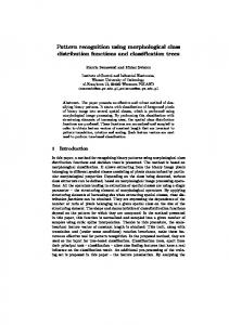
Figure 1: Geometric interpretation of equation 5.2. Note that W and Ti span the invariance manifold, d is the Euclidean distance between the pattern X and the centroid W, and net D ( D1T-sided )2 is the one-sided tangent distance.

internal parameters (weights). SpeciŽcally, it is characterized by a set of n C 1 vectors of the same dimension as the input vectors. One vector (W ) is used as the reference vector (centroid), while the remaining vectors fT 1 , . . . , T n g are used as tangent vectors. Moreover, the set of tangent vectors constitutes an orthonormal basis. This set of parameters is organized in such a way as to form a tangent model. Formally, the net input of a TD-Neuron for a pattern k is netk D min kM ( µ ) ¡ X k k2 C b,

µ

(5.1)

where b is the offset. A good model should return small net input for patterns belonging to the learned class. Since the tangent vectors constitute an orthonormal basis, equation 5.1 can exactly and easily be computed by using the projections of the input vector over the model subspace (see Figure 1):

netk D k X k ¡ W k2 ¡ | {z }

dk

n X iD1

[(X k ¡ W )t T i ]2 C b

Discriminant Pattern Recognition

D dtk dk ¡

n X iD1

1361

[ dtk T i ]2 C b, | {z }

(5.2)

c ik

where, for the sake of notation, dk denotes the difference between the input pattern X k and the centroid W , and the projection of dk over the ith tangent vector is denoted by c ik . Note that the right side of equation 5.2 mainly involves dot products, just as in a standard neuron. The output of the TD-Neuron is then computed by transforming the net through a nonlinear monotone function f . In our experiments, we have used the symmetric sigmoidal function ok D

2 ¡ 1. 1 C enetk

(5.3)

We have used a monotonic decreasing function so that the output corresponding to patterns belonging to the target class will be close to 1. 5.1 Training the TD-Neuron. A discriminant model based on the TDNeuron can be obtained by adapting equation 4.1. Given a training set f(X 1 , t1 ), . . . , ( X N , tN )g, where

»

ti D

1 ¡1

if X i 2 C if X i 2 C

is the ith desired output for the TD-Neuron, and N D NC C NC is the total number of patterns in the training set, an error function can be deŽned as

ED

N 1X ( tk ¡ o k ) 2 , 2 D1

(5.4)

k

where ok is the output of the TD-Neuron for the kth input pattern. Equation 5.4 can be written into a form similar to equation 4.1 by making explicit the target values ti , by splitting the sum in such a way to group together patterns belonging to C and patterns belonging to C, and by weighting the negative examples with a constant l ¸ 0:

2 3 NC NC X 1 X 2 2 (1 ¡ ok ) C l (1 C oj ) 5 . ED 4 2 kD1 jD1

In our experiments we have chosen l D

NC , NC

(5.5)

thus balancing the strength

of patterns belonging to C and those belonging to C.

1362

D. Sona, A. Sperduti, and A. Starita

Using equations 5.2 and 5.3, it is trivial to compute the changes for the centroid, the tangent vectors, and the offset by using a gradient-descent approach over equation 5.5: " !#

D W D ¡g D T i D ¡g

¡ @E ¢ @W

D ¡2 g

@T i

D ¡2 g

¡ @E ¢

D b D ¡gb

¡ @E ¢ @b

D gb

N X

kD1

N £ X kD1

N X

kD1

(

(tk ¡ ok ) fk0 dk ¡ ( tk ¡ ok ) fk0 c ik dk

[(tk ¡ ok ) fk0 ]

¤

n X

c ik T i

(5.6)

iD1

(5.7)

(5.8)

ok where g and gb are learning parameters, and fk0 D @@net . k Before training the TD-Neuron by gradient descent, however, the tangent subspace dimension must be decided. To solve this problem, we developed a constructive algorithm that adds tangent vectors one by one, according to computational needs. This idea is also justiŽed by the observation that using equations 5.6 through 5.8 leads to the sequential convergence of the tangent vectors according to their relative importance. This means that in the Žrst approximation, all the tangent vectors remain random vectors while the centroid converges Žrst. Then one of the tangent vectors converges to the most relevant transformation (while the remaining tangent vectors are still immature), and so on until all the tangent vectors converge, one by one, to less and less relevant transformations. This behavior suggests starting the training using only the centroid (i.e., without tangent vectors) and then adding tangent vectors as needed. Under this learning scheme, since there are no tangents when the centroid is computed, equation 5.6 becomes

D W D ¡g

¡ @E ¢ @W

D ¡2g

N X kD1

[(tk ¡ ok ) fk0 dk ].

(5.9)

The constructive algorithm has two phases (see Table 1). First is the centroid computation, based on the iterative use of equations 5.8 and 5.9. Then the centroid is frozen, and one by one all tangent vectors T i are trained using equations 5.7 and 5.8. At each iteration in the learning phase, the tangent vector T i must be orthonormalized with respect to the already computed tangent vectors. 3 If after a Žxed number of iterations (we have used 300 iterations) the total error variation is less than a Žxed threshold (0.01%) and no change in the classiŽcation performance over training set occurs, a new tangent vector is added. The tangent vectors are iteratively added until changes in the classiŽcation accuracy become irrelevant. 3

The computational complexity of the orthonormalization is linear in the number of already computed tangent vectors.

Discriminant Pattern Recognition

1363

Table 1: Constructive Algorithm for the TD-Neuron. Initialize the centroid W. Update b and W by equations 5.8 and 5.9 until they converge. Freeze W. REPEAT .

Initialize a new tangent vector Ti . Update Ti and b with equations 5.7 and 5.8, and orthonormalize Ti with respect to f T1 , . . . , Ti¡1 g until it converges. Freeze Ti . UNTIL new Ti gives little accuracy changes.

The initialization of internal vectors of the TD-Neuron can be done in many different ways. On the basis of empirical evidence, we have concluded that the learning phase of the centroid can be considerably reduced by initializing the centroid with the mean value of the patterns belonging to the positive class. We have also devised a “good” initialization algorithm for tangent vectors (see Table 2) that tries to minimize the drop in the net input for all the patterns due to the increase in the tangent subspace dimension (see Figure 2). This is obtained by introducing a new tangent vector that mainly spans the residual subspace between the patterns in the positive class and the current model. In this way, patterns that are in the negative class will be only mildly affected by the new introduced tangent vector. We have also devised a “better ” initialization algorithm based on principal components of difference vectors for all classes. However, the observed training speed-up is not justiŽed by the additional computational overhead due to SVD computation needed at each tangent vector insertion. In our experiments, we have also used a simple form of regularization over the parameters (weight decay with penalty equal to 0.997, i.e., all paTable 2: Initialization Procedure for the Tangent Vectors. • For each class c 2 (C [ C), compute the mean value of differences between patterns and model: dc D

1 Nc

P Nc

p D1

(Xp ¡ M(h )).

• Orthonormalize the vector dc of the class C with respect to the mean values of differences of all other classes belonging to C, and return it as the new initial tangent vector.

1364

D. Sona, A. Sperduti, and A. Starita

Figure 2: Total error variation during learning phase for pattern 0. At each new tangent insertion, there is a reduction of the distance between patterns and the model (also for patterns belonging to class C). This affects the output of the neuron for all patterns, increasing the total output squared error.

rameters are multiplied by the penalty before adding the gradient), obtaining a better convergence. 6 Results

In order to obtain comparable results, we had to use the same number of parameters for all algorithms. In particular, for tangent-based algorithms, the number of vectors is given by the number of tangent vectors incremented by 1 (the centroid). For this reason, the LVQ algorithms are compared to tangent distance-based algorithms using a number of reference vectors equal to the number of tangent vectors plus 1. Furthermore, with the two-sided HSS algorithm, we also have to consider the tangent vectors corresponding to the input patterns. SpeciŽcally, we used six transformations (tangent vectors) for each input pattern: clockwise and counterclockwise rotations and translation in the four cardinal directions.4 We tested our constructive algorithm versus the two versions of the HSS algorithm and LVQ algorithms in the LVQ PAK package (Kohonen, Hynni4

We preferred to approximate the exact tangents by Žnite differences; in this way, the local shape of the manifold is interpolated in a better way.

Discriminant Pattern Recognition

1365

nen, Kangas, Laaksonen, & Torkkola, 1996) (optimized-learning-rate LVQ1, original LVQ1, LVQ2.1, LVQ3), using 10,704 binary digits taken from the NIST-3 data set. The binary 128 £ 128 digits were transformed into 64-gray level 16 £16 images by a simple local counting procedure.5 The only preprocessing transformation performed was the elimination of empty borders. The training set consisted of 5000 randomly chosen digits; the remaining digits were used in the test set. For each tangent distance algorithm, a single tangent model for each class of digit was computed. With the LVQ algorithms, a set of reference vectors was used for each class; the number of reference vectors was chosen so as to have as many parameters as in the tangent distance algorithms. In particular, we tested all algorithms based on tangent distance using a different number of vectors for each experiment, starting from 1 vector per class (centroid without tangent vectors) up to 16 vectors per class (centroid plus 15 tangent vectors). The number of reference vectors for LVQ algorithms has been chosen accordingly. Concerning LVQ algorithms, here we report just the results obtained by using LVQ2.1 with 1-NN based on Euclidean distance as the classiŽcation rule, since this algorithm reached the best performance over an extended set of experiments involving LVQ algorithms with different settings for the learning parameters. The classiŽcation of the test digits was performed using the label of the closest model for HSS, the 1-NN rule for LVQ algorithms, and the highest output for the TD-Neuron algorithm. For the sake of comparison, we also performed a classiŽcation using the nearest-neighbor rule (1-NN) with the Euclidean distance as classiŽcation metric. In this case, we classiŽed each pattern by looking at the label of the nearest vector in the learning set. In Figure 3 we report the results obtained on the test set for different numbers of tangent vectors for all models. The best classiŽcation result (96.84%) was given by 1-NN with Euclidean distance, followed by the two-sided HSS with 9 tangent vectors (96.6%). 6 With the same number of parameters (15 tangent vectors), the TD-Neuron and the one-sided HSS gave a performance rate of 96.51% and 96.42%, respectively. Finally, LVQ2.1 obtained a performance rate of 96.48% using 15 vectors per class. From these results, it can be noted that the two-sided HSS algorithm does overŽt the data after the ninth tangent vector; this is not true for the remaining algorithms. Nevertheless, all the models reach a similar performance with the same number of parameters, which is slightly below the performance attained by the 1-NN classiŽer using Euclidean distance. However, both the tangent models and LVQ algorithms have the advantage of being less demanding in both space and response time than 1-NN.

5 The original image is partitioned into 16 £ 16 windows and the number of pixel with value equal to 1 is used as the gray value for the corresponding pixel in the new image. 6 There are also six tangent vectors corresponding to the input pattern.

1366

D. Sona, A. Sperduti, and A. Starita

Figure 3: Results obtained on the test set by models generated by both versions of HSS, LVQ2.1, TD-Neuron, and 1-NN with Euclidean distance.

It is interesting that the recognition performance of the TD-Neuron system is basically monotone in the number of parameters (tangent vectors), while all other methods present overŽtting and high variance in the results. Although from Figure 3 it seems that the tangent models and LVQ2.1 are equivalent, when introducing a rejection criterion the model generated by the TD-Neuron outperforms the other algorithms (see Figure 4). We used the same rejection criterion for all algorithms. A pattern is rejected when the difference between the Žrst- and the second-best outputs belonging to different classes is less than a Žxed threshold.7 Furthermore, introducing the rejection criterion also leads to the surprising result that the one-sided version of HSS performs better than the two-sided version. In order to assess whether the better performance exhibited by the TDNeuron was due to the speciŽc rejection criterion or the discriminant capability of the model, we performed some experiments using a different rejection criterion: reject when the best output value is smaller (TD-Neuron) or greater (HSS, LVQ and 1-NN) than a threshold. In Figure 5 we report the curves obtained for the best models—TD-Neuron and one-sided HSS— with, for comparison, the corresponding curves of Figure 4. These results demonstrate that the improvement shown by the TD-Neuron is not tight to a speciŽc rejection criterion. Moreover, removing the

7

Obviously the threshold is different for each algorithm.

Discriminant Pattern Recognition

1367

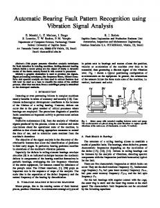
Figure 4: Error-rejection curves for all algorithms: one-sided HSS with 15 tangent vectors, two-sided HSS with 9 and 15 tangent vectors, TD-Neuron with 9 and 15 tangent vectors, LVQ2.1 with 15 reference vectors, and 1-NN with Euclidean distance. The boxed diagram shows a detail of the curves demonstrating that the TD-Neuron with 15 tangent vectors has the best trade-off between error and rejection.

sigmoidal function from the TD-Neuron during the test phase, the rejection curves does not change signiŽcantly for both rejection criteria. Thus, we can conclude that the improvement of the TD-Neuron is mainly due to the discriminant training procedure. In Figure 6, four examples of TD-Neuron models are reported. In the left-most column, the centroids of patterns 0, 1, 2, and 3 are shown. The remaining columns contain the Žrst (and most important) four tangent vectors for each model. 7 Discussion and Conclusion

We introduced the TD-Neuron, which implements the one-sided version of the tangent distance, and gave a constructive learning algorithm for building a tangent subspace with discriminant capabilities. There are many advantages to using the proposed computational model versus the HSS model and LVQ algorithms. SpeciŽcally, we believe that the proposed approach is particularly useful in applications where it is very important to have a classiŽcation system that is both discriminant and fast in recognition.

1368

D. Sona, A. Sperduti, and A. Starita

Figure 5: Detail of error-rejection curves of one-sided HSS and TD-Neuron for two different rejection criteria: threshold on the output absolute value (abs) and threshold on the difference between the best and the second-best output models (diff). The curves for the TD-Neuron model with removed nonlinear output are individuated by the additional label (linear).

We also compared the TD-Neuron constructive algorithm to two different versions of the HSS algorithm, the LVQ2.1 algorithm and the 1-NN classiŽcation criterion. The obtained results over the NIST-3 database of handwritten digits show that the TD-Neuron is superior to the HSS algorithms based on singular value decomposition and the LVQ algorithms, since it reaches a better trade-off between error and rejection. Moreover, we have assessed that the better trade-off is mainly due to the discriminant capabilities of our model. Concerning the proposed neural formulation, we believe that the nonlinear sigmoidal transformation is useful since removing it and using the ( )) for training would drastically reduce the size of the inverted target (o¡1 k tk space of solutions in the weight space. In fact, very high or very low values for the net input would not minimize the error function with the inverted target, while being fully acceptable in the proposed model. Moreover, the nonlinearity increases the stability of learning because of the saturated output. During the model generation, for a Žxed number of tangent vectors, the HSS algorithm is faster than ours because it needs only a fraction of the training examples (only one class). However, our algorithm is remarkably more efŽcient than HSS algorithms when a family of tangent models, with an increasing number of tangent vectors, must be generated. Also the LVQ

Discriminant Pattern Recognition

1369

Figure 6: Tangent models obtained by the TD-Neuron for digits 0, 1, 2, and 3. The centroids are shown in the left-most column; the remaining columns show the Žrst four tangent vectors.

algorithms are faster than TD-Neuron, but they have as a drawback a poor rejection performance. An additional advantage of the TD-Neuron model is that because the training algorithm is based on a gradient-descent technique, several TDNeurons can be arranged to form a hidden layer in a feedforward network with standard output neurons, which can be trained by a trivial extension of backpropagation. This may lead to a remarkable increase in the transformation-invariant features of the system. Furthermore, it should be possible to extract information easily from the network regarding the most important features used during classiŽcation (see Figure 6). References Hastie, T., Simard, P. Y., & S¨ackinger, E. (1995). Learning prototype models for tangent distance. In G. Tesauro, D. S. Touretzky, & T. K. Leen (Eds.), Advances in neural information processing systems, 7 (pp. 999–1006). Cambridge, MA: MIT Press. Hinton, G. E., Dayan, P., & Revow, M. (1997). Modeling the manifold of images of handwritten digits. IEEE Transactions on Neural Networks, 8, 65–74.

1370

D. Sona, A. Sperduti, and A. Starita

Kohonen, T., Hynninen, J., Kangas, J., Laaksonen, J., & Torkkola, K. (1996). LVQ PAK: The learning vector quantization program package (Tech. Rep. No. A30). Espoo, Finland: Helsinki University of Technology, Laboratory of Computer and Information Science. Available online at: http://www.cis.hut.Ž/ nnrc/nnrcc-programs.html. Schwenk, H., & Milgram, M. (1995a). Learning discriminant tangent models for handwritten character recognition. In International Conference on ArtiŽcial Neural Networks (pp. 985–988). Berlin: Springer-Verlag. Schwenk, H., & Milgram, M. (1995b).Transformation invariant autoassociation with application to handwritten character recognition. In G. Tesauro, D. S. Touretzky, & T. K. Leen (Eds.), Advances in neural information processing systems, 7 (pp. 991–998). Cambridge, MA: MIT Press. Simard, P. Y. (1994). EfŽcient computation of complex distance metrics using hierarchical Žltering. In J. D. Cowan, G. Tesauro, and J. Alspector (Eds.), Advances in neural information processing systems, 6 (pp. 168–175). San Mateo, CA: Morgan Kaufmann. Simard, P. Y., LeCun, Y., & Denker, J. (1993). EfŽcient pattern recognition using a new transformation distance. In S. J. Hanson, J. D. Cowan, & C. L. Giles (Eds.), Advances in neural information processing systems, 5 (pp. 50–58). San Mateo, CA: Morgan Kaufmann. Sona, D., Sperduti, A., & Starita, A. (1997). A constructive learning algorithm for discriminant tangent models. In M. C. Mozer, M. I. Jordan, & T. Petsche (Eds.), Advances in neural information processing systems, 9 (pp. 786–792). Cambridge, MA: MIT Press. Sperduti, A., & Stork, D. G. (1995). A rapid graph-based method for arbitrary transformation-invariant pattern classiŽcation. In G. Tesauro, D. S. Touretzky, and T. K. Leen (Eds.), Advances in neural information processing systems, 7 (pp. 665–672). Cambridge, MA: MIT Press. Received April 7, 1998; accepted April 8, 1999.