criminative training, log-linear model, conditional random field. 1. INTRODUCTION. State-of-the-art speech recognition systems are based on discrimi-.
DISCRIMINATIVE HMMS, LOG-LINEAR MODELS, AND CRFS: WHAT IS THE DIFFERENCE? G. Heigold, S. Wiesler, M. Nußbaum-Thom, P. Lehnen, R. Schl¨uter, and H. Ney Human Language Technology and Pattern Recognition Computer Science Department, RWTH Aachen University, Aachen, Germany {heigold,wiesler,nussbaum,lehnen,schlueter,ney}@cs.rwth-aachen.de ABSTRACT Recently, there have been many papers studying discriminative acoustic modeling techniques like conditional random fields or discriminative training of conventional Gaussian HMMs. This paper will give an overview of the recent work and progress. We will strictly distinguish between the type of acoustic models on the one hand and the training criterion on the other hand. We will address two issues in more detail: the relation between conventional Gaussian HMMs and conditional random fields and the advantages of formulating the training criterion as a convex optimization problem. Experimental results for various speech tasks will be presented to carefully evaluate the different concepts and approaches, including both a digit string and large vocabulary continuous speech recognition tasks. Index Terms— speech recognition, hidden Markov model, discriminative training, log-linear model, conditional random field 1. INTRODUCTION State-of-the-art speech recognition systems are based on discriminative Gaussian HMMs (GHMMs). The major points of criticism of this conventional approach are the indirect parameterization of the posterior model including many parameter constraints, the nonconvexity of the conventional training criteria such that the optimization can get stuck in local optima, and the insufficient flexibility of the HMMs to incorporate additional dependencies and knowledge sources. The log-linear framework addresses these issues in a principled way. Examples for this framework include the log-linear model, the maximum entropy Markov model (MEMM) [1], the conditional random field (CRF) [2, 3], the hidden CRF (HCRF) [4, 5], and the conditional augmented (C-Aug) models [6]. In the log-linear approach, the posterior is directly modeled, the traditional training criterion is convex (except for HCRFs and C-Aug models), and it is easy to incorporate additional knowledge (although possibly at the cost of increased complexity) [7]. Various approaches to direct acoustic modeling have been investigated. HCRFs [4] are closest to GHMMs. Linear-chain HCRFs [4, 5] differ from conventional GHMMs mainly in the model parameterization. The training criterion for HCRFs is non-convex like for GHMMs. If all hidden variables are eliminated (cf. mixtures) or suppressed (cf. alignments), the HCRF reduces to a CRF [2, 3] and the optimization problem is convex. MEMMs [1] are similar to CRFs but the posterior is based on a different decomposition and different dependence assumptions. Alternatively, a hybrid architecture [8] with log-linear models to represent the HMM state posteriors can be used. All these convex approaches have in common that the decision boundary is linear and thus, the choice of features is essential for a
good separation of the data. The features considered so far in the literature can be roughly divided into simple generic features (cf. kernel) [1, 2, 5, 9], and more sophisticated features to overcome the limitations of conventional GHMMs (e.g. detector features) [3, 7, 10]. More sophisticated features tend to be more powerful than the simple generic features, possibly at the risk of outsourcing the main work into a separate preprocessing step. A pseudo log-linear approach was proposed in [6]. This (non-convex) approach also estimates some parameters of the features and thus, may alleviate the feature selection problem. The remainder of this paper is organized as follows. Section 2 introduces the models under consideration. It also formulates an equivalence relation for Gaussian and log-linear HMMs. Section 3 defines the different training criteria used in this paper. The focus will be on convex optimization techniques for speech recognition. Section 4 provides experimental results to study numerical issues of the parameterization of the models and the utility of convex optimization in speech recognition. Section 5 offers concluding remarks. 2. MODELS Assume a sequence of feature vectors x1T = (x1 , . . . , xT ) ∈ T D and a word sequence W = w1N = (w1 , . . . , wN ). Conventional speech recognition systems are decomposed into the language model and the acoustic model. The language model typically is an m-gram language model while the acoustic model is based on GHMMs. The acoustic model introduces the HMM state sequences sT1 = (s1 , . . . , sT ) to further decompose the acoustic model into the transition and the emission models. The latter model is traditionally represented by Gaussian mixture models. Under these assumptions, the joint probability of x1T and W reads pGHMM,θ (x1T , W) = (1) N T XY Y p(wn |wn−1 ) p(s |st−1 , W) N(xt |µ st W , Σ) . | {z } T t=1 | t {z } | {z } n=1 language model s1
transition model
emission model
For simplicity, a bigram language model and single Gaussians N(x|µ sW , Σ) with mean µ sW ∈ D and a globally pooled covariance matrix Σ ∈ D×D are used. The model parameters of this GHMM are θ := {p(w|v) ∈ + , p(s|s0 , W) ∈ + , µ sW ∈ D , Σ ∈ D×D } subject to the usual constraints, e.g. normalization of (conditional) probabilities and positive-definiteness of covariance matrix. The joint probability in Equation (1) induces the string posterior by Bayes rule pGHMM,θ (W|x1T )
=
pGHMM,θ (x1T , W) . P pGHMM,θ (x1T , V) V
(2)
HCRFs are CRFs with hidden variables. Log-linear HMMs (LHMMs) are linear-chain HCRFs sharing the model structure with GHMMs where a log-linear parameterization for the generative submodels are used [4] pLHMM,Λ (W|x1T ) = (3) N T XY 1 Y exp(αw w ) exp(α s s W ) exp(α st W + λ>st W xt ) . ZΛ (x1T ) n=1 | {zn−1 n} T t=1 | {zt−1 t } | {z } language model
s1
transition model
emission model
ZΛ (x1T ).
Unlike the The normalization constant is denoted by GHMM parameters, the LHMM parameters are unconstrained, Λ := {αvw ∈ , α s0 sW ∈ , α sW ∈ , λ sW ∈ D }. It was shown in [4] that the GHMM in Equation (1) can be transformed into an LHMM in Equation (3) with identical posteriors. Due to the parameter constraints of GHMMs, it is in general not straightforward to transform the LHMM in Equation (3) into a valid GHMM in Equation (1). Using the ambiguity of the LHMM parameters and the propagation of the normalization constants, the parameter constraints of GHMMs can be imposed on the LHMM such that this transformation is always possible [11]. This implies that the LHMM posterior model in Equation (3) and the posterior model induced by GHMMs in Equation (2) are equivalent, i.e., the associated sets of posteriors are identical [11]. The equivalence relation was experimentally verified on a simple concept tagging task including a bigram concept model [11]. This result can be extended to Gaussian mixture models by redefining the HMM state sequence network to include the density indices, and to density-specific covariance matrices by adding second order features to the LHMM. The equivalence relation for GHMMs and LHMMs implies that all posteriorbased algorithms perform equally for either posterior model. The discriminative training criteria are an example for posterior-based algorithms, which are discussed next. 3. TRAINING CRITERIA The above models are usually optimized by maximizing the mutual information, i.e., the log-posteriors (MMI). Depending on the precise definition of the posteriors, different variants of MMI can be derived. To simplify notation, the language model, the transition model, and the emission model in Equations (1) and (3) are denoted by the (pseudo) probabilities h(W), gΛ (s0 , s), and fΛ (x, s), respectively. The explicit dependence of f, g on W is dropped because it is not used. This convention leads to the decision rule T Y ˆ . h(W) f (xt , st )g(st−1 , st ) W = arg max max W sT 1 t=1
It is independent of the model and the training criterion. Conventional lattice-based MMI training uses word lattices D to approximate the normalization constant for the string posterior. In addition, the maximum approximation is assumed such that each hypothesis in the word lattice uniquely defines an HMM state sequence. The numerator lattice N is the set of HMM state sequences representing the correct word sequence. These assumptions lead to the string posterior used for MMI training T P Q h(W(sT1 )) fΛ (xt , st )g(st−1 , st ) p(lattice) (W|x1T ) Λ
=
sT1 ∈N
P sT1 ∈D
t=1
h(W(sT1 )) sT1
T Q t=1
numerator of the posterior, and the incomplete sum for the normalization constant in combination with realignment. This conventional training criterion can be made convex, i.e., the HCRF is cast into a CRF, by replacing the normalization constant with the sum over the complete set of HMM state sequences S and by using only the best HMM state sequence sˆT1 representing W in the numerator (to be determined by some existing acoustic model)
.
(4)
fΛ (xt , st )g(st−1 , st )
The word sequence associated with is denoted by W(sT1 ). This choice of the posterior results in a non-convex training criterion, both for GHMMs and HCRFs. This is due to the sum in the
p(Λf ool−proo f ) (W|x1T ) =
h(W( sˆT1 )) P sT1 ∈S
T Q t=1
h(W(sT1 ))
fΛ (xt , sˆt )gΛ ( sˆt−1 , sˆt )
T Q t=1
.
(5)
fΛ (xt , st )gΛ (st−1 , st )
This training criterion is referred to as fool-proof MMI. It is convex because it has the same functional structure as a CRF and allows for the optimization of all model parameters, (hopefully) without any approximations and heuristics. Due to the summation over all HMM state sequences, this approach is feasible only for small tasks (e.g. digit strings). For larger tasks, we adopt the hybrid approach [8] to optimize the emission parameters in Equation (3). Here, log-linear models instead of neural networks or support vector machines are taken as the static classifiers. All other parameters cannot be optimized in this approach. This simplification considerably speeds up the training. Similar to fool-proof MMI, the best HMM state sequence sˆT1 is assumed to be known and kept fixed during training. The symbol posterior includes the HMM state prior p(s) (e.g. relative frequencies) p(Λf rame) ( sˆt |xt )
=
p( sˆt ) fΛ (xt , sˆt ) P . p(s) fΛ (xt , s)
(6)
s
The induced frame-based MMI training criterion is convex. Several refinements to MMI are considered for the experiments in Section 4. First, `2 -regularization is used. Furthermore, the posteriors can be scaled by some γ ∈ + , and a margin term scaled with some ρ ∈ + can be incorporated into standard MMI. These modifications are implemented by replacing the posterior in Equation (6) with, for instance, [p( sˆt ) fΛ (xt , sˆt ) exp(−ρδ( sˆt , sˆt ))]γ f rame) . p(Λ,γρ ( sˆt |xt ) = P [p(s) fΛ (xt , s) exp(−ρδ(s, sˆt ))]γ s
This variant of MMI is called modified/margin-based MMI (MMMI). For lattice-based (Equation (4)) and fool-proof (Equation (5)) MMI, the posterior can be modified in a similar way to derive the respective M-MMI training criterion. For segment-based MMI, the Hamming accuracy instead of the Kronecker delta is used in the margin term. The convexity is not affected by the margin term. It was shown in [12] that for ρ = 1, the resulting training criterion Fγ(M−MMI) converges to the optimization problem of SVMs using γ→∞
the hinge loss function F (S V M) , Fγ(M−MMI) → F (S V M) . Finally, other (in general non-convex) training criteria can be used for the optimization as well, e.g. minimum phone error (MPE). 4. EXPERIMENTAL RESULTS This section provides experimental comparisons of discriminative HMMs, log-linear models, and CRFs for different speech tasks. Unless otherwise stated, the training criteria are optimized with Rprop [13]. 4.1. Tasks & Setups Special about the RWTH maximum likelihood (ML) GHMM baseline models is that they use globally pooled variances. This allows us to produce rather good ML baseline systems with a fairly high number of Gaussian densities.
from scratch
German digit strings. The SieTill corpus consists of continuously spoken German digits recorded over the telephone line from adult speakers. The recognition system is based on gender-dependent whole-word HMMs. The front-end consists of conventional cepstral features (MFCC) without derivatives. A sliding window of size five is used to include temporal context. The feature vector is projected to 25 dimensions by means of a linear discriminant analysis (LDA). See [14] for further details. The corpus statistics and setup are summarized in Table 1. American English read speech. The Wall Street Journal (WSJ) corpora include American English read speech recorded under clean conditions. Since the official WSJ0 corpus does not provide a development set, 410 sentences were extracted from ten new speakers of the North American Business (NAB) task and used as the development set. The same setup as in [9] is used for the experiments. The front-end consists of MFCC features which are normalized by a fast variant of vocal tract length normalization (VTLN). A trigram language model is used for recognition. More details on the corpus statistics and the setup can be found in Table 1. Mandarin broadcasts. This large vocabulary continuous speech recognition task consists of Mandarin broadcasts news (BN) and conversations (BC). The experiments are based on the same setup as described in [12] and summarized in Table 1. The BNBC Cn system uses PLP features augmented with a voicing feature. Nine consecutive frames are concatenated. A tonal feature with its first and second derivatives and neural network (NN) based features are added. The feature vector is then projected to 45 dimensions by means of speaker adaptive training (SAT) and constrained maximum likelihood linear regression (CMLLR). The PLP features are warped using VTLN. For recognition, a 4-gram language model is used. 4.2. Parameterization & numerical issues GHMM vs. LHMM. It was shown in theory that GHMMs and LHMMs are equivalent, see Section 2. Nevertheless, LHMMs may outperform GHMMs in practice [4] due to numerical issues or the approximate equivalence (e.g. if only the emission model is reestimated). Table 2 provides an experimental comparison of GHMMs and LHMMs for the SieTill and the BNBC Cn tasks. The ML GHMM baseline systems were optimized with expectationmaximization (EM). These models were used to initialize the discriminative training for GHMMs and LHMMs. The discriminative training was done using extended Baum-Welch (EBW, only GHMMs) and Rprop (GHMMs and LHMMs). So far, we have not observed any consistent differences between GHMMs and LHMMs in practice. Density-specific variances. Unlike most other groups, we use a single globally pooled diagonal covariance matrix. Could we do better with density-specific diagonal covariance matrices? LHMMs with first order features xd and second order features xd2 are equivalent to GHMMs with density-specific diagonal covariance matrices (see Section 2). This observation allows us to test GHMMs with
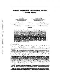
5 4.5 from ML 4 WER [%]
Table 2. Word error rates (WER) for SieTill and BNBC Cn test corpora. M-MMI and MPE is used for SieTill and BNBC Cn. WER [%] SieTill BNBC Cn Model Criterion Optim. Test Eval06 Eval07 GHMM ML EM 1.8 17.9 11.9 M-MMI EBW 1.7 17.0 11.2 or Rprop 1.6 16.5 11.1 LHMM MPE 1.6 16.2 10.8
frame-based M-MMI lattice-based M-MMI fool-proof M-MMI
3.5 3 2.5 from frame 2 1.5 0
50
100
150 200 iteration index
250
300
Fig. 1. Word error rate (WER) vs. iteration index on SieTill test corpus. Convergence is not reached after 200 iterations in general. specific covariance matrices without changing our software. The experimental results on BNBC Cn suggest that second order features do not help regarding WER but tended to converge faster than the system with first order features only. 4.3. Convex optimization Implementation checking. The definition of a fool-proof training algorithm as discussed in Section 3 allows for the optimization of all model parameters from scratch in a principled way. Here, we check how well the theoretical expectations carry over to practice. Figure 1 illustrates the convergence behavior of the different training criteria for different initializations of the training. The convergence rate tends to be lower for lattice-based MMI than for framebased and fool-proof MMI, in particular when initialized from ML. The word error rates (WERs) after convergence are: frame-based M-MMI: 1.9% (from scratch), 1.9% (from ML, single densities); lattice-based M-MMI: 4.5% (from scratch), 2.0% (from ML, single densities), 1.8% (from frame-based M-MMI); fool-proof M-MMI: 1.8% (from scratch), 1.6% (from frame-based M-MMI). Due to the assumptions made to derive the convex training criteria (see Section 3), special attention is directed to the following issues. First, the dependence on the model initialization. It appears from Figure 1 that frame-based MMI is independent of the initialization. In contrast, fool-proof MMI shows some weak dependence on the initialization. This might indicate some problems with the numerical stability of fool-proof MMI, e.g. flat optimum. As expected, lattice-based MMI which is non-convex strongly depends on the choice of the initialization. Second, the correlation of the training criterion and test WER because the assumptions (e.g. the discrimination of HMM state sequences rather than word sequences) may affect the performance of the training criterion. Frame-based MMI tends to perform slightly worse than lattice-based and fool-proof MMI which perform equally. Finally, the sensitivity to the HMM state alignment. This might be an issue in particular if the log-linear model/CRF cannot be initialized with the corresponding GHMM as e.g. in [2]. The experiments do not suggest that this is a critical issue. Feasibility and utility of higher order features. Table 3 studies the effect of higher order features, again on the simple German digit string recognition task. The systems including higher order features up to degree one, two, and three have 11k, 151k, and 1,407k parameters, respectively. The error rate for a discriminative GHMM with 715k parameters is also shown in Table 3 for comparison. Higher order features beyond degree three are not feasible. For larger tasks like for example WSJ0, already the use of third order features leads to rather high training times while the second order features are limited regarding WER. So, additional features are considered next.
Identifier (description) SieTill (German digit strings) WSJ0 (American read speech) BNBC Cn (Mandarin BN&BC)
Table 1. Speech corpora and setups. Vocabulary size Audio data [h] #States/#Dens. 11 11.3 (Train)/ 11.4 (Test) 430/430-27k 5k 15 (Train)/0.4 (Test) 1,500/220k 60k 1,500 (Train) 4,500/1,200k 2.2 (Eval06)/2.9 (Eval07)
Table 3. Word error rates (WERs) on SieTill test corpus for higher order features, frame-based M-MMI (’frame’, convex) vs. latticebased M-MMI (’lattice’, non-convex). Model Criterion xd xd xd0 xd xd0 xd00 Log-linear model frame 3.0 1.9 1.8 Log-linear model lattice 2.7 1.8 1.5 GHMM (27k dens.) lattice 1.6 N/A N/A Set up of a log-linear model from scratch. Finally, a log-linear model is set up for the WSJ0 task [9]. The emission features include cluster features (cf. radial basis function kernel) [2, 9] in addition to the higher order features (cf. polynomial kernel). Assuming clusters µl and cluster priors p(l) from a preprocessing step, the cluster feaP tures are defined as p(l)N(x|µl , Σ)/ l0 p(l0 )N(x|µl0 , Σ). The cluster features have the advantage of being sparse, i.e., only a few cluster features are active (i.e., above some small positive threshold) at the same time. This makes the accumulation of the sufficient statistics considerably more efficient, even for a large number of features. The baseline model uses first order features and 130 monophonebased HMM states only. Then, the model complexity is increased step by step by using second order features, cluster features including temporal context, and CART-tied HMM states in addition. The results are shown in Table 4. The log-linear system was trained from scratch, starting with the alignment from the linear segmentation. To train the final system, a few realignments were required. Table 4. WER for log-linear models on the WSJ0 test corpus. Feature setup WER [%] First order features 22.7 +second order features 10.3 +210 cluster features + temporal context of size 9 6.2 +1,500 CART-tied HMM states 3.9 +realignment 3.6 GHMM (ML/MMI) 3.6/3.0 5. CONCLUSION Several aspects in the context of direct acoustic modeling were studied. Gaussian and log-linear HMMs are equivalent. In spite of this, the log-linear parameterization might be numerically more stable as it avoids the estimation of covariance matrices, for instance. An experimental comparison of these models for a digit string recognition task and a large vocabulary speech recognition task suggested that this is not the case. Nevertheless, the log-linear framework is attractive due to its simple and flexible parameterization which will considerably simplify the incorporation of additional dependencies and knowledge sources in the future. The convexity of the training criteria is another issue often addressed in numerical optimization. Under a few assumptions, the conventional training criterion in speech recognition can be made convex. First experimental results along this line are encouraging as for the convergence behavior, including the stability and the initialization but are less efficient than the conventional training criteria. Finally, a log-linear model for a continuous speech recognition task was set up from scratch (i.e., no existing GHMM used at all) to evaluate the effectiveness of the direct modeling approach.
Features/Setup 25 LDA(MFCC) 33 LDA(MFCC)+VTLN 45 SAT/CMLLR(PLP+voicing +3 tones+32 NN)+VTLN
6. ACKNOWLEDGMENTS This work was partly realized as part of the Quaero Programme, funded by OSEO, French State agency for innovation, and it was partly funded by the European Union under the integrated project LUNA (FP6-033549). 7. REFERENCES [1] H.-K. J. Kuo and Y. Gao, “Maximum entropy direct models for speech recognition,” IEEE Transactions on Audio, Speech and Language Processing, vol. 14, no. 3, 2006. [2] Y. H. Abdel-Haleem, Conditional random fields for continuous speech recognition, Ph.D. thesis, Faculty of Engineering, University of Sheffield, Sheffield, UK, 2006. [3] J. Morris and E. Fosler-Lussier, “CRANDEM: conditional random fields for word recognition,” in Interspeech, Brighton, England, Sept. 2009. [4] A. Gunawardana, M. Mahajan, A. Acero, and J.C. Platt, “Hidden conditional random fields for phone classification,” in Interspeech, Lisbon, Portugal, Sept. 2005. [5] D. Yu, L. Deng, and A. Acero, “Using continuous features in the maximum entropy model,” Pattern Recognition Letters, 2009. [6] M.I. Layton and M.J.F. Gales, “Augmented statistical models for speech recognition,” in ICASSP, Toulouse, France, May 2006. [7] G. Heigold, G. Zweig X. Li, , and P. Nguyen, “A flat direct model for speech recognition,” in ICASSP, Taipei, Taiwan, Apr. 2009. [8] T. Robinson, M. Hochberg, and S. Renals, “The use of recurrent networks in continuous speech recognition,” in Automatic Speech and Speaker Recognition, K. K. Paliwal C.-H. Lee, F. K. Soong, Ed. Kluwer Academic Publishers, Norwell, MA, USA, 1996. [9] S. Wiesler, M. Nußbaum-Thom, G. Heigold, R. Schl¨uter, and H. Ney, “Investigations on features for log-linear acoustic models in continuous speech recognition,” in ASRU, Merano, Italy, Dec. 2009. [10] G. Zweig and P. Nguyen, “Maximum mutual information multi-phone units in direct modeling,” in Interspeech, Brighton, England, Sept. 2009. [11] G. Heigold, P. Lehnen, R. Schl¨uter, and H. Ney, “On the equivalence of Gaussian and log-linear HMMs,” in Interspeech, Brisbane, Australia, Sept. 2008. [12] G. Heigold, T. Deselaers, R. Schl¨uter, and H. Ney, “Modified MMI/MPE: A direct evaluation of the margin in speech recognition,” in ICML, Helsinki, Finland, July 2008. [13] M. Riedmiller and H. Braun, “A direct adaptive method for faster backpropagation learning: The Rprop algorithm,” in ICNN, San Francisco, CA, USA, 1993. [14] G. Heigold, D. Rybach, R. Schl¨uter, and H. Ney, “Investigations on convex optimization using log-linear HMMs for digit string recognition,” in Interspeech, Brighton, England, Sept. 2009.