Distance-Constraint Reachability Computation in ... - VLDB Endowment

Distance-Constraint Reachability Computation in ∗ Uncertain Graphs Ruoming Jin† † Kent State University Kent, OH, USA {jin, lliu}@cs.kent.edu

Lin Liu†

Bolin Ding‡ ‡ UIUC Urbana, IL, USA [email protected]

Haixun Wang§ § Microsoft Research Asia Beijing, China [email protected]

ABSTRACT Driven by the emerging network applications, querying and mining uncertain graphs has become increasingly important. In this paper, we investigate a fundamental problem concerning uncertain graphs, which we call the distance-constraint reachability (DCR) problem: Given two vertices s and t, what is the probability that the distance from s to t is less than or equal to a user-defined threshold d in the uncertain graph? Since this problem is #P-Complete, we focus on efficiently and accurately approximating DCR online. Our main results include two new estimators for the probabilistic reachability. One is a Horvitz-Thomson type estimator based on the unequal probabilistic sampling scheme, and the other is a novel recursive sampling estimator, which effectively combines a deterministic recursive computational procedure with a sampling process to boost the estimation accuracy. Both estimators can produce much smaller variance than the direct sampling estimator, which considers each trial to be either 1 or 0. We also present methods to make these estimators more computationally efficient. The comprehensive experiment evaluation on both real and synthetic datasets demonstrates the efficiency and accuracy of our new estimators.

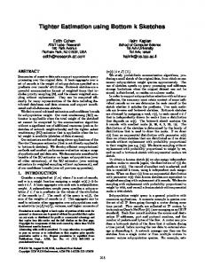
(a) Uncertain Graph G .

(b) G1 with 0.0009072.

(c) G2 with 0.0009072.

(d) G3 with 0.0006048.

Figure 1: Running Example. vertex can reach another one, is the basis for a variety of databases (XML/RDF) and network applications (e.g., social and biological networks) [8, 22]. For uncertain graphs, reachability is not a simple Yes/No question, but instead, a probabilistic one. Specifically, reachability from vertex s to vertex t is expressed as the overall probability of those possible graphs of G in which s can reach t. For uncertain graph G in Figure 1, we can see that s can reach t in its possible graphs G1 and G2 but not in G3 ; if we enumerate all the possible graphs of G and add up the weights of those possible graphs where s can reach t, we get s can reach t with probability 0.5104. The simple reachability in uncertain graphs has been widely studied in the context of network reliability and system engineering [5]. In this paper, we investigate a more generalized and informative distance-constraint reachability (DCR) query problem, that is: Given two vertices s and t in an uncertain graph G, what is the probability that the distance from s to t is less than or equal to a user-defined threshold d? Basically, the distance-constraint reachability (DCR) between two vertices requires them not only to be connected in the possible graphs, but also to be close enough. For the example in Figure 1, if the threshold d is selected to be 2, then, t is considered to be unreachable from 2 in G2 (under this distance constraint). Clearly, DCR query enables a more informative categorization and interrogation of the reachability between any two vertices. At the same time, the simple reachability also becomes a special case of the distance-constraint reachability (considering the case where the threshold d is larger than the length of the longest path, or simply the sum of all edge weights in G). Distance-constraint reachability plays an important and even critical role in a wide range of applications. In a variety of real-world emerging communication networks, DCR is essential for analyzing their reliability and communication quality. For instance, in peerto-peer (P2P) networks, such as Freenet and Gnutella [4, 11], the communication between two nodes is only allowed if they are separated by a small number of intermediate hops (to avoid congestion). In such situation, as the uncertain graph naturally models the link failure probability, the DCR query serves as the basic tool to in-

1. INTRODUCTION Querying and mining uncertain graphs has become an increasingly important research topic [13, 24, 25]. In the most common uncertain graph model, edges are independent of one another, and each edge is associated with a probability that indicates the likelihood of its existence [13, 24]. This gives rise to using the possible world semantics to model uncertain graphs [13, 1]. A possible graph of an uncertain graph G is a possible instance of G. A possible graph contains a subset of edges of G, and it has a weight which is the product of the probabilities of all the edges it has. For example, Figure 1 illustrates an uncertain graph G, and three of its possible graphs G1 , G2 and G3 , each with a weight. A fundamental question for uncertain graphs is to categorize and compute reachability between any two vertices. In a deterministic directed graph, the reachability query, which asks whether one ∗

R. Jin and L. Liu were partially supported by the National Science Foundation, under CAREER grant IIS-0953950. Permission to make digital or hard copies of all or part of this work for personal or classroom use is granted without fee provided that copies are not made or distributed for profit or commercial advantage and that copies bear this notice and the full citation on the first page. To copy otherwise, to republish, to post on servers or to redistribute to lists, requires prior specific permission and/or a fee. Articles from this volume were invited to present their results at The 37th International Conference on Very Large Data Bases, August 29th - September 3rd 2011, Seattle, Washington. Proceedings of the VLDB Endowment, Vol. 4, No. 9 Copyright 2011 VLDB Endowment 2150-8097/11/06... $ 10.00.

551

d, we say vertex t is d-reachable from s if the distance from s to t in G is less than or equal to d.

terrogate the probability whether one node can communicate with another, and to study the network reliability in general. Indeed, such diameter-constrained (or hop-constrained) reliability has been proposed in the context of communication network reliability [12] though its computation remains difficult. Recently, there have been efforts to model the road network as an uncertain graph due to the unexpected traffic jam [7]. Here, each link in the road network can be weighted using the distance or the travel time between them. In addition, a probability can be assigned to model the likelihood of a traffic jam. Given this, one of the basic problems is to determine the probability whether the travel distance (or travel time) from one point to another is less than or equal to a threshold considering the uncertainty issue. Clearly, this directly corresponds to a DCR query. The DCR query can also be applied to trust analysis in social networks. Specifically, in a trust network, one person can trust another with a probabilistic trust score. When two persons are not directly connected, the trust between them can be modeled by their distance (the number of hops between them). In particular, a real world study [17] finds that people tend to trust others if they are connected through some trust relationship; however, the number of hops between them must be small. Thus, given a trust radius, which constrains how far away can a trusted person be, the likelihood that the distance between one person to another is within this radius can be used to evaluate the trust between those non-adjacent pairs. In the uncertain graph terminology, this is a DCR query.

D EFINITION 1. (s-t distance-constraint reachability) Computing s-t distance-constraint reachability in an uncertain graph G is to compute the probability of the possible graphs G, in which vertex t is d-reachable from s, where d is the distance constraint. Specifically, let ( 1, if dis(s, t|G) ≤ d d Is,t (G) = 0, otherwise Then, the s-t distance-constraint reachability in uncertain graph G with respect to parameter d is defined as X d (1) Rds,t (G) = Is,t (G) · Pr[G] . G⊑G

Note that the problem of computing s-t distance-constraint reachability is a generalization of computing s-t reachability without the distance-constraint, which is often referred to as the two-point reliability problem [14]. Simply speaking, it computes the total sampling probability of possible graphs G ⊑ G, in which vertex t is reachable from vertex s. Using the aforementioned distanceconstraint reachabilityPnotation, we may simply choose an upper bound such as W = e∈E w(e) (the total weight of the graph as an example), and then RW s,t (G) becomes simple s-t reachability. Computational Complexity and Estimation Criteria The simple s-t reachability problem is known to be #P-Complete [21, 2], even for special cases, e.g., planar graphs and DAGs, and so is its generalization, s-t distance-constraint reachability. Thus, we cannot expect the existence of a polynomial-time algorithm to find the exact value of Rds,t (G) unless P =N P . The distance-constraint reachability problem is much harder than the simple s-t reachability problem as we have to consider the shortest path distance between s and t in all possible graphs. Indeed, the existing s-t reachability computing approaches have mainly focused on the small graphs (in the order of tens of vertices) and cannot be directly extended to our problem. Given this, the key problem this paper addresses is how to efficiently and accurately approximate the s-t distance-constraint reachability online. Now, let us look at the key criteria for evaluating the quality of b an approximate approach (or the quality of an estimator). Let R d b be a general estimator for Rs,t (G). Intuitively, R should be as close to Rds,t (G) as possible. Mathematically, this property can be b − Rds,t (G))2 , captured by the mean squared error (MSE), E(R which measures the expected difference between an estimator and the true value. It can also be decomposed into two parts:

1.1 Problem Statement Uncertain Graph Model: Consider an uncertain directed graph G = (V, E, p, w), where V is the set of vertices, E is the set of edges, p : E → (0, 1] is a function that assigns each edge e a probability that indicates the likelihood of e’s existance, and w : E → (0, ∞) associates each edge a weight (length). Note that we assume the existence of an edge e is independent of any other edges. In our example (Figure 1), we assume each edge has unit-length (unit-weight). Let G = (VG , EG ) be the possible graph which is realized by sampling each edge in G according to the probability p(e) (denoted as G ⊑ G). Clearly, we have EG ⊆ E and the possible graph G has Pr[G] sampling probability: Y Y Pr[G] = p(e) (1 − p(e)). e∈EG

e∈E\EG

m

There are a total of 2 possible graphs (for each edge e, there b or not). In our example (Figure 1), are two cases: e exists in G graph G has 29 possible graphs, and as an example for the graph sampling probability, we have

b − Rds,t (G))2 E(R

Pr[G1 ] = p(s, a)p(a, b)p(a, t)p(s, c)(1 − p(s, b))(1 − p(b, t)) × (1 − p(s, c))(1 − p(b, c))(1 − p(c, b)) = 0.0009072

= =

b + (E(R) b − Rds,t (G))2 V ar(R) b + (BiasR) b 2 V ar(R)

An estimator is unbiased if the expectation of the estimator is b = 0), i.e., E(R) b = Rds,t (G) (for equal to the true value (BiasR b measures the our problem). The variance of estimator V ar(R) average deviation from its expectation. For an unbiased estimator, the variance is simply the MSE. In other words, the variance of an unbiased estimator is the indicator for measuring its accuracy. In addition, the variance is also frequently used for constructing the confidence interval of an estimate for approximation and the smaller the variance, the more accurate confidence interval estimate we have [18]. All estimators studied in this paper will be proven to be the unbiased estimators of Rds,t (G). Thus, the key criterion to discriminate them is their variance [18, 6].

Distance-Constraint Reachability: A path from vertex v0 to vertex vp in G is a vertex (or edge) sequence (v0 , v1 , · · · , vp ), such that (vi , vi+1 ) is an edge in EG (0 ≤ i ≤ p − 1). A path is simple if no vertex appears more than once in the sequence. To study distance-constraint reachability in uncertain graph, only simple paths need to be considered. Given two vertices s and t in G, a path starting from s and ending at t is referred to as an s-t-path. We say vertex t is reachable from vertex s in G if there is an s-t-path in G. The distance or length of an s-t-path is the sum of the lengths of all the edges on the path. The distance from s to t in G, denoted as dis(s, t|G), is the distance or length of the shortest path from s to t, i.e., minimal length of all s-t-paths. Given distance-constraint

552

2.2

Besides the accuracy of the estimator, the computational efficiency of the estimator is also important. This is especially important for online answering s-t distance-constraint reachability query. In sum, in this paper, our goal is to develop an unbiased estimator of Rds,t (G) with minimal variance and low computational cost. Minimal DCR Equivalent Subgraph: Before we proceed, we note that given vertices s and t, only subsets of vertices and edges in G are needed to compute the s-t distance-constraint reachability. Specifically, given vertices s and t, the minimal equivalent DCR subgraph Gs = (Vs , Es , p, w) ⊆ G where Vs

=

{v ∈ V |dis(s, v|G) + dis(v, t|G) ≤ d},

Es

=

{e = (u, v) ∈ E|dist(s, u|G) + w(e) + dis(v, t|G) ≤ d}.

Path-Based Approach

In this subsection, we introduce the paths (or cuts) based approach for estimating Rds,t (G). To facilitate our discussion, we first formally introduce d-path from s to t. A s-t path in G with length less than or equal to distance constraint d is referred to as d-path between s and t. The d-path is closely related to the s-t distanceconstraint reachability: If vertex t is d-reachable from vertex s in a graph G, i.e., dis(s, t|G) ≤ d, then, there is a d-path between s and t. If not, i.e., dis(s, t|G) > d, then, for any s-t path in G, its length is higher than d (there is no d-path). Given this, the complete set of all d-paths in G (the complete possible graph with respect to G which includes all the edges in G), denoted as P = {P1 , P2 , · · · , PL }, can be used for computing the s-t distance-constraint reachability:

Here, G is the complete possible graph with respect to G which includes all the nodes and edges in G. Basically, Vs and Es contain those vertices and edges that appear on some s-t paths whose distance is less than or equal to d. Clearly, we have Rds,t (Gs ) = Rds,t (G). A fast linear method can help extract the minimal equivalent DCR subgraph (See Appendix A). Since we only need to work on Gs , in the remainder of the paper, we simply use G for Gs when no confusion can arise.

Rds,t (G) = Pr[P1 ∨ P2 · · · ∨ PL ] = −

X

L

X

Pr[Pi ]

Pr[Pi ∩ Pj ] + · · · + (−1) πPr[P1 ∩ P2 · · · ∩ PL ]

i6=j

Given this, we can apply the Monte-Carlo algorithm proposed in [9] to estimating Pr[P1 ∨ P2 · · · ∨ PL ] within absolute error ǫ with probability at least 1 − δ. In sum, the path-based estimation approach contains two steps: 1) Enumerating all d-paths from s to t in G (See Subsection E.1); 2) Estimating Pr[P1 ∨ P2 · · · ∨ PL ] using the Monte-Carlo algorithm [9]. b P , which is an unbiased estimator This estimator, denoted as R of Rds,t (G) [9], has the following variance as [6]:

2. BASIC MONTE-CARLO METHODS In this section, we will introduce two basic Monte-Carlo methods for estimating Rds,t (G), the s-t distance-constraint reachability.

2.1 Direct Sampling Approach A basic approach to approximate the s-t distance-constraint reachability is using sampling: 1) we first sample n possible graphs, G1 , G2 , · · · , Gn of G according to edge probability p; and 2) we then compute the shortest path distance in each sample graph Gi , b B) and thus Ids,t (Gi ). Given this, the basic sampling estimator (R is: Pn d i=1 Is,t (Gi ) bB = Rds,t (G) ≈ R n b B is an unbiased estimator of The basic sampling estimator R b B ) = Rds,t (G). the s-t distance-constraint reachability, i.e., E(R Its variance can be simply written as [6]

L X b P ) = 1 Rds,t (G)( V ar(R Pr[Pi ] − Rds,t (G)) n i=1

P Thus, depending on whether L i=1 Pr[Pi ] is bigger than or less b than 1, the variance of RP can be bigger or smaller than that of b B . The key issue of this approach is the computational requireR ment to enumerate and store all d-paths between s and t. This can be both computationally and memory expensive (the number of dpaths can be exponential). Can we derive a faster and more accurate estimator for Rds,t (G) b B and R b P ? In the next section, we than these two estimators, R provide a positive answer to this question.

b B (1 − R b B) b B ) = 1 Rds,t (G)(1 − Rds,t (G)) ≈ 1 R V ar(R n n The basic sampling method can be rather computationally expensive. Even when we only need to work on the minimal DCR equivalent subgraph Gs , its size can be still large, and in order to generate a possible graph G, we have to toss the coin for each edge in Es . In addition, in each sampled graph G, we have to invoke the shortest path distance computation to compute Ids,t (G), which again is costly. We may speedup the basic sampling methods by extending the shortest-path distance method, like Dijkstra’s or A∗ [15] algorithm for sampling estimation. Recall that in both algorithms, when a new vertex v is visited, we have to immediately visit all its neighbors (corresponding to visiting all outgoing edges in v) in order to maintain their corresponding estimated shortest-path distance from the source vertex s. Given this, we may not need to sample all edges at the beginning, but instead, only sample an edge when it will be used in the computational procedure. Specifically, only when a vertex is just visited, we will sample all its adjacent (outgoing) edges; then, we perform the distance update operations for the end vertices of those sampled edges in the graph; we will stop this process either when the targeted vertex t is reached or when the minimal shortest-distance for any unvisited vertex is more than threshold d. A similar procedure on Dijkstra’s algorithm is applied in [13] for discovering the K nearest neighbors in an uncertain graph.

3.

NEW SAMPLING ESTIMATORS

In this section, we will introduce new estimators based on unequal probability sampling (UPS) and an optimal recursive sampling estimator. To achieve that, we will first introduce a divideand-conquer strategy which serves as the basis of the fast computation of s-t distance constraint reachability (Subsection 3.1).

3.1

A Divide-and-Conquer Exact Algorithm

Computing the exact s-t distance-constraint reachability (Rds,t (G)) is the basis to fast and accurately approximate it. The naive algorithm to compute Rds,t (G) is to enumerate G ⊑ G, and in each G, compute shortest path distance between s and t to test whether d(s, time of this algorithm is “ t|G) ≤ d. The total running ” O 2|E| (|E| + |V | log |V |) assuming Dijkstra algorithm is used

for distance computation1 . Here, we introduce a much faster exact algorithm to compute Rds,t (G). Though this algorithm still has the exponential computational complexity, it significantly reduces our search space by avoiding enumerating 2m possible graphs of G. The basic idea is to recursively partition all (2m ) possible graphs 1

553

Here, G is actually the minimal DCR equivalent subgraph Gs .

of G into the groups so that the reachability of these groups can be computed easily. To specify the grouping of possible graphs, we introduce the following notation:

will invoke the procedure R(G, ∅, ∅). Based on the factorization lemma (Lemma 1), this procedure first partitions the entire set of possible graphs of uncertain graph G into two parts (prefix groups) using any edge e in G:

D EFINITION 2. ((E1 , E2 )-prefix group) The (E1 , E2 )-prefix group of possible graphs from uncertain graph G, which is denoted as G(E1 , E2 ), includes all the possible graphs of G which contains all edges in edge set E1 ⊆ E and does not contain any edge in edge set E2 ⊆ E, i.e., G(E1 , E2 ) = {G ⊑ G|E1 ⊆ EG ∧ E2 ∩ EG = ∅}. We refer to E1 and E2 as the inclusion edge set and the exclusion edge set, respectively.

Rds,t (G(∅, ∅)) = p(e)Rds,t (G({e}, ∅))+(1−p(e))Rds,t (G(∅, {e})). Then, it applies the same approach to partition each prefix group recursively (Line 6 − 7) until either E1 contains a d-path or E2 contains a d-cut (Line 1 − 5) in the prefix group G(E1 , E2 ). The computational process of the recursive procedure R can be represented in a full binary enumeration tree (Figure 2 (a)). In the tree, each node corresponds to a prefix group G(E1 , E2 ) (also an invoke of the procedure R). Each internal node has two children, one corresponding to including an uncertain edge e, another excluding it. In other words, the prefix group is partitioned into two new prefix groups: G(E1 ∪ {e}, E2 ) and G(E1 , E2 ∪ {e}). Further, we may consider each edge in the tree is weighted with probability p(e) for edge inclusion and 1 − p(e) for edge exclusion. In addition, the leaf node can be classified into two categories, L which contains all the leaf nodes with E1 containing a d-path, and L which contains the remaining leaf nodes, i.e., all those leaf nodes with E2 include a d-cut. Note that any uncertain edge e can be selected for each prefix group (in Line 6) without affecting the correctness of the recursive procedure. However, it does affect its computational complexity, which is determined by average recursive depth (average prefixlength), i.e., the average number of edges |E1 ∪ E2 | we have to select in order to determine whether t is d-reachable from s for all the possible graphs in the prefix group. If the average recursive depth is a, then, a total of O(2a ) prefix groups need to be enumerated, which can be significantly smaller than the complete O(2m ) possible graphs of G. An uncertain edge selection approach in Section E is provided to minimize the average recursive depth.

Note that for a nonempty prefix group, the inclusion edge set E1 and the exclusion edge set E2 are disjoint (E1 ∩ E2 = ∅). In Figure 1, if we want to specify those possible graphs which all include edge (s, a) and do not contain edges (s, b) and (b, t), then, we may refer those graphs as ({(s, a)}, {(s, b), (b, t)})-prefix group. To facilitate our discussion, we introduce the generating probability of the prefix group G(E1 , E2 ) as: Y Y (1 − p(e)) p(e) Pr[G(E1 , E2 )] = e∈E1

e∈E2

This indicates the overall sampling probability of any possible graph in the prefix group. Given this, the s-t distance-constraint reachability of a (E1 , E2 )prefix group is defined as X Pr[G] Rds,t (G(E1 , E2 )) = Ids,t (G) · (2) Pr[G(E1 , E2 )] G∈(G(E1 ,E2 ))

Basically, it is the overall likelihood that t is d-reachable from s conditional on the fixed prefix G(E1 , E2 ). It is easily derived that Rds,t (G) = Rds,t (G(∅, ∅)). The following lemma characterizes the s-t distance-constraint reachability of (E1 , E2 )-groups and forms the basis for its efficient computation. Its proof is omitted for simplicity. L EMMA 1. (Factorization Lemma) For any (E1 , E2 )-prefix group of uncertain G and any uncertain edge e ∈ E\(E1 ∪ E2 ), Rds,t (G(E1 , E2 ))

=

p(e)Rds,t (G(E1 ∪ {e}, E2 ))

+

(1 − p(e))Rds,t (G(E1 , E2 ∪ {e})).

3.2

Unequal Probability Sampling Framework

Now, we study an estimation framework of Rds,t (G) using the unequal probability sampling scheme [18] based on Algorithm 1. Unequal Probability Sampling (UPS) Framework: To estimate Rds,t (G), we apply the unequal sampling scheme: 1) each leaf node in the enumeration tree (Figure 2 (a)) is associated with a leaf weight: the generating probability of the corresponding prefix group, Pr[G(E1 , E2 )]; and 2) each leaf node G(E1 , E2 ) in the enumeration tree is sampled with a leaf sampling probability q(G(E1 , E2 )), where the sum of all leaf sampling probability (q(G(E1 , E2 )) is 1. Note that in the UPS framework, the leaf sampling probability q can be different from the leaf weight. Given this, we now study the well-known unequal sampling estimator, the Hansen-Hurwitz estimator [18]: assuming we sampled n leaf nodes, 1, 2, · · · , n, in the enumeration tree, and let P ri be the weight associated with the i-th sampled leaf node and let qi be the leaf sampling probability, then the Hansen-Hurwitz estimator b HH ) for Rds,t (G) is: (denoted as R

In addition, for any (E1 , E2 )-prefix group of uncertain G, if E1 contains a d-path from s to t, then, Rds,t (G(E1 , E2 )) = 1; if E2 contains a d-cut 2 between s and t, then, Rds,t (G(E1 , E2 )) = 0. Also, E1 containing a d-path and E2 containing a d-cut cannot be both true at the same time though both can be false at the same time. Algorithm 1 R(G, E1 , E2 ) Parameter: G: Uncertain Graph; Parameter: E1 : Inclusion Edge List; Parameter: E2 : Exclusion Edge List; 1: if E1 contains a d-path from s to t then 2: return 1; 3: else if E2 contains a d-cut from s to t then 4: return 0; 5: end if 6: select an edge e ∈ E\(E1 ∪ E2 ) {Find a remaining uncertain edge} 7: return p(e)R(G, E1 ∪ {e}, E2 ) + (1 − p(e))R(G, E1 , E2 ∪ {e})

n X P ri Ids,t (G) b HH = 1 R n i=1 qi

(3)

In other words, we may consider each leaf node in L contributes P ri and each leaf node in L contributes 0 to the estimation. It is b HH ) is an unbiased easy to show the Hansen-Hurwitz estimator (R d estimator for Rs,t (G), and its variance can be derived as

Algorithm 1 describes the divide-and-conquer computation procedure for Rds,t (G) based on Lemmas 1. To compute Rds,t (G), we 2

b HH ) = V ar(R

An edge set Cd of G is a d-cut between s and t if G\Cd has a distance greater than d, i.e., dis(s, t|G\Cd ) > d.

554

X P ri 1 X − Rds,t (G))2 + ( qi Rds,t (G)2 ) qi ( n i∈L qi i∈L

(a) Enumeration Tree of Recursive Computation of Rds,t (G). (b) Divide and Conquer. Figure 2: Divide-and-Conquer method. Applying the Lagrange method, we can easily find that the opb HH ) is timal sampling probability for minimal variance V ar(R b HH ) = achieved when qi = P ri , and the minimal variance is V ar(R d d 1 R (G)(1 − R (G)). In other words, the best leaf sampling s,t s,t n b HH is the one equal probability q to minimize the variance of R to the leaf weight in L! Note that this is consistent with the general UPS theory which suggests the sampling probability should be proportional to the corresponding sampling weight [18]. Given this, we can sample a leaf node in the enumeration tree as follows: Simply tossing a coin at each internal node in the enumeration tree to determine whether the uncertain edge e (also corresponding to Line 6 in Algorithm 1) should be included (in E1 ) with probability q(e) = p(e) or excluded (in E2 ) with probability 1 − p(e); continuing this process until a leaf node is reached. Basically, we perform a random walk starting from the root node and stopping at the leaf node in the enumeration tree (Figure 2 (a)), and at each internal node, we randomly goes to its left (selecting the edge e) with probability p(e) or goes to its right (excluding edge e) with probability 1 − p(e). Such random walk sampling can guarantee that the leaf sampling probability is equal to the corresponding leaf weight! Due to space limitation, the pseudocode of the random b HH is sketched in Appendix C. walk sampling scheme for R Interestingly, we note this UPS estimator is equivalent to the direct sampling estimator, as each leaf node is counted as either 1 or b HH = R b B . In other words, the di0 (like Bernoulli trial): R rect sampling scheme is simply a special (and optimal) case of the Hassen-Hurvitz estimator! This leads to the following observation: b HH ) or direct samfor any optimal Hassen-Hurvitz estimator (R b B ), their variance is only determined by n and pling estimator (R has no relationship to the enumeration tree size. This seems to be rather counter-intuitive as the smaller the tree-size (or the smaller number of the leaf nodes), the better chance (information) we have for estimating Rds,t (G). A Better UPS Estimator: Now, we introduce another UPS estib HT ), which can provide mator, the Horvitz-Thomson estimator (R b HH and the smaller variance than the Hansen-Hurvitz estimator R b direct sampling estimator RB under mild conditions. Assuming we sampled n leaf nodes in the enumeration tree and among them there are l distinctive ones 1, 2, · · · , l (l is also referred to as the effective sample size), let the leaf inclusion probability πi be probability to include leaf i in the sample, which is define as πi = 1 − (1 − qi )n where qi is the leaf sampling probability. The Horvitz-Thomson estimator for Rds,t (G) is: ˆ HT = R

l X P ri Ids,t (G) i=1

πi

ˆ HT ) is an unbiased estimator for the popuThomson estimator (R lation total (Rds,t (G)). Its variance can be derived as follows [18], where πij is the probability that both leafs i and j are included in the sample: πij = 1 − (1 − qi )n − (1 − qj )n + (1 − qi − qj )n : b HT ) V ar(R

=

X „ 1 − πi «

P ri2 πi X „ πij − πi πj « P ri P rj . πi πj i,j∈L,i6=j i∈L

+

Using Taylor expansions and Lagrange method, we can find the minimal variance can be approximated when qi = P ri . This basically suggests the similar leaf sampling strategy (the random walk from the root to the leaf) for the Hansen-Hurwitz estimator can be applied to the Horvitz-Thomson estimator as well. However, different from the Hansen-Hurwitz estimator, the Horvitz-Thomson estimator utilizes each distinctive leaf once. Though in general the variances between the Hansen-Hurwitz estimator and the HorvitzThomson estimator are not analytically comparable, in our treebased sampling framework and under reasonable approximation, we are able to prove the latter one has smaller variance. b HT ) ≤ V ar(R b HH )) When for any samT HEOREM 1. (V ar(R 2 b HH )−V ar(R b HT )=Ω(P ple leaf node i, nP ri ≪ 1, V ar(R i∈L P ri ).

The proof of this theorem can be found in Appendix B. This result suggests that for small sample size n and/or when the generating probability of the leaf node is very small, then the HorvitzThomson estimator is guaranteed to have smaller variance. In Section 4, the experimental results will further demonstrate the effectiveness of this estimator. A reason for this estimator to be effective is that it directly works on the distinctive leaf nodes which partly reflect the tree structure. In the next subsection, we will introduce a novel recursive estimator which more aggressively utilizes the tree structure to minimize the variance.

3.3

Optimal Recursive Sampling Estimator

In this subsection, we explore how to reduce the variance based on the factorization lemma (Lemma 1). Then, we will describe a novel recursive approximation procedure which combines the deterministic procedure with the sampling process to minimize the estimator variance. Variance Reduction: Recall that for the root node in the enumeration tree, we have the following results based on the the factorization lemma (Lemma 1): Rds,t (G) = p(e)Rds,t (G({e}, ∅)) + (1 − p(e))Rds,t (G(∅, {e}))

.

To facilitate our discussion, let τ = Rds,t (G), τ1 = Rds,t (G({e}, ∅)) and τ2 = Rds,t (G(∅, {e})).

Note that if qi is very small, then πi ≈ nqi . The Horvitz-

555

Algorithm 2 OptEstR(G, E1 , E2 , n)

Now, instead of directly sampling all the leaf nodes from the root (like suggested in last subsection), we consider to estimate both τ1 and τ2 independently, and then combine them together to estimate τ . Specifically, for n total leaf samples, we deterministically allocate n1 of them to the left subtree (including edge e, τ1 ), and n2 of them to the right subtree (excluding edge e, τ2 ); then, we can apply b HH , or equivthe aforementioned sampling estimators, such as R b b b alently RB ), to both subtrees. Let R1 and R2 be the estimators for τ1 (left subtree) and τ2 (right subtree), respectively. Thus, the combined estimator for Rds,t (G) is b = p(e)R b 1 + (1 − p(e))R b2 R

Parameter: E1 : Inclusion Edge List; Parameter: E2 : Exclusion Edge List; Parameter: n: sample size; 1: if n ≤ threshold {Stop recursive sample allocation} then b HH (G, E1 , E2 , n); {apply non-recursive sampling esti2: return R mator} 3: end if 4: if E1 contains a d-path from s to t then 5: return 1; 6: else if E2 contains a d-cut from s to t then 7: return 0; 8: end if 9: select an edge e ∈ E\(E1 ∪ E2 ) {Find a remaining uncertain edge} 10: return p(e)OptEstR(G, E1 ∪ {e}, E2 , ⌊np(e)⌋)+ (1 − p(e))OptEstR(G, E1 , E2 ∪ {e}, n − ⌊np(e)⌋);

(4)

b 1 and R b2 Clearly, this combined estimator is unbiased as both R are unbiased estimators for τ1 and τ2 , respectively. Why this might be a better way to estimate Rds,t (G)? Intuitively, this is because we eliminate the “uncertainty” of edge e from the estimation equation. Of course, the important question is how such elimination can benefit us, and to answer this, we need address this problem: what are the optimal sample allocation strategy to minimize the overall estimator variance? The variance of the combined estimator depends on the variance of the two individual estimators (they are independent and their covariance is 0):

Table 1: Relative Error (in %)

15-25 26-35 35-45 45-55

bB R 1.00 1.00 1.00 1.00

bD R B 3.00 2.80 1.75 1.42

bP R 0.98 1.50 1.17 1.59

b HT R 0.90 1.08 1.77 1.39

b RHH R 0.96 0.90 1.36 1.33

b RHT R 0.71 0.72 1.33 1.30

Table 2: Relative Variance Efficiency

b = p(e)2 V ar(R b 1 ) + (1 − p(e))2 V ar(R b 2) V ar(R) τ (1 − τ ) τ (1 − τ2 ) 1 1 2 = p(e)2 + (1 − p(e))2 n1 n2

When τ1 and τ2 are known, we clearly can find the optimal sample allocation (n1 and n2 are functions of τ1 and τ2 ) for minimizb However, in this problem, such prior knowledge is ing V ar(R). clearly unavailable. Given this, can we still allocate samples to reduce the variance? An interesting discovery we made is when the sample size allocation is proportional to the edge inclusion probability, i.e., n1 = p(e)n and n2 = (1 − p(e))n, the variance of the b HH ) = τ (1−τ ) original optimal Hassen-Hurvitz estimator V ar(R n can be reduced!

bD R B 0.81 0.77 0.58 0.73

bP R 0.15 0.44 0.58 0.82

b HT R 0.12 0.23 0.45 0.80

b RHH R 0.12 0.27 0.23 0.44

b RHT R 0.08 0.17 0.20 0.43

Table 3: Query Time (in ms) 15-25 26-35 35-45 45-55

R∗ 2 53 1828 91748

bB R 314 358 314 344

bD R B 314 345 313 345

bP R 532 564 535 565

b HT R 193 233 234 251

b RHH R 11 20 23 23

b RHT R 15 34 42 45

sample size is very small, all the non-recursive sampling estimab HT , R b HH , and R b B , all become equivalent. tors, including R The computational complexity of this recursive sampling estimator is O(na), where a is the average recursive depth or the average length from the root node to the leaf node in the enumeration tree. But it tends to be more computationally efficient than the UPS b HH and R b HT . This is because the recursively samestimators R pling estimator visits the upper-part of the enumeration tree (for the recursive sample size allocation) only once and does not need perform any coin-toss for the each node at this part of the tree. However, the UPS estimators have to perform coin-toss for each node and may repetitively revisit the same node in the upper-level of the tree, where this new estimator visits each node only once. Finally, we note that the analytically comparison between the varib HT and the recursively ance of the Horvitz-Thomson estimator R b is not conclusive (See further analysis in Appendix D), estimator R though the experimental evaluation demonstrates the superiority of the new sampling estimator (Section 4).

T HEOREM 2. (Variance Reduction) When, n1 = p(e)n and b ≤ V ar(R b HH ), and more specifically, n2 = (1−p(e))n, V ar(R) the variance is reduced by b HH ) − V ar(R) b = V ar(R

15-25 26-35 36-45 46-55

bB R 3.42 2.52 2.30 1.79

p(e)(1 − p(e))(τ1 − τ2 )2 . n

For its simplicity, we omit the proof for the above theorem. Recall τ1 is the overall probability of those leaf nodes in the left subtree (G({e}, ∅)) and in L, i.e., when edge e is included and t is d-reachable from s and τ2 is the overall probability of those possible graphs where e is excluded. Clearly, when edge e is included, the probability for t is d-reachable from s is greater. Especially, this theorem suggests the bigger the impact for edge e being included or excluded, the greater the variance reduction effect (directly proportional to (τ1 −τ2 )2 ). In addition, this sample size allocation method can be generalized and applied at the root node of any subtree in the enumeration tree for reducing the variance. Recursive Sampling Estimator: Given this, we introduce our reb R , which is outlined in Algorithm 2. cursive sampling estimator R Basically, it follows the exact computational recursive procedure (Algorithm 1) and recursively split the sample size n to ⌊np(e)⌋ and n − ⌊np(e)⌋ for estimating Rds,t (G(E1 ∪ {e}, E2 )) and Rds,t (G(E1 , E2 ∪ {e})), respectively (Line 10). In addition, when the sample size n is smaller than the threshold (typically the threshold is very small, less than 5), we can avoid the recursive allocation by perform the direct sampling (Line 1 and 2). Note that when the

4.

EXPERIMENTAL EVALUATION

In the experimental study, we will focus on studying the accuracy and computational efficiency of different sampling estimators on both synthetic and real datasets. Specifically, the sampling estimab B : this is the direct sampling estimator using A∗ tors include: 1) R algorithm for searching shortest path distance [15]. The sampling process is also combined with the search process to maximize its bD computational efficiency; 2) R B : we apply a state-of-the-art varib B to ance reduction method, Dagger Sampling [10, 6], on top of R b boost the estimation accuracy; 3) RP : this is the path-based esti-

556

mator based on [9] which needs to enumerate all the d-paths from b HT : this is the Horvitz-Thomson estimator based on the s to t; 4) R b RHH : this is the unequal probabilistic sampling framework; 5) R optimal recursive sampling estimator OptEstR and when the number of samples in the recursive sampling process is less than the b HH threshold (set to be 5), the non-recursive sampling estimator R b RHT : this is the opti(Hansen-Hurwitz estimator) is used; 6) R mal recursive sampling estimator OptEstR and when the number of samples in the recursive sampling process is less than the threshold b HT (Horvitz-Thomson (5), the non-recursive sampling estimator R estimator) is used. For all the last three estimators, they all utilize the FindDPath procedure to select the next edge in the recursive b HH computation procedure. In addition, we omit the results for R (Hansen-Hurwitz estimator) because it is equivalent to the direct b B. sampling estimator R To compare the accuracy of these different sampling estimators, we utilize two criteria: the relative error and the estimation variance. For the relative error, we apply R∗ procedure to compute the exact distance-constraint reachability. Let R be the exact result and b be the estimation result. Then, the relative error ǫ is computed as R b ǫ = |R−R| . For the estimation variance, for each query, we will run R each estimator K times, and thus, we have 100 different estimating b1 ,R b2 , · · · , R bK (in this work, we set K = 100). The results: R PK b i −R)2 (R . Here R estimation variance σ is estimated as: σ = i=1K−1 PK b is the estimation average ( i=1 Ri )/K. The computational efficiency is evaluated by the running time of each estimator. All algorithms are implemented by using C++ and the Standard Template Libaray (STL) and were conducted on a 2.0GHz Dual Core AMD Opteron CUP with 4.0GB RAM running Linux.

Table 4: Relative Error with Real Graphs (in %) bB R bD R bP b HT b RHH R b RHT R R R B 4.40 3.23 1.66 1.71 1.94 1.74 3.85 3.47 1.36 2.22 2.21 1.73 3.62 3.22 1.40 1.92 2.08 1.64 Table 5: Query Time with Real Graphs (in Seconds) bB bD bP b HT b RHH R b RHT R R R R R B DBLP 51.65 55.50 5915.12 26.08 5.93 10.08 Yeast PPI 1.15 1.97 4959.37 0.50 0.11 0.21 Fly PPI 2.55 4.77 215.98 1.13 0.45 0.67 DBLP Yeast PPI Fly PPI

4.1 Experimental Results on Synthetic Datasets We first report the experimental results on synthetic uncertain graphs. Here, the graph topologies are generated by either Erd¨osR´enyi random graph model or power law graph generator [3]. The edge weight is randomly generated between 1 to 100 according to uniform distribution. The edge probability is randomly generated between 0 to 1 according to uniform distribution. Random Graph: In this experiment, we generate an Erd¨os-R´enyi random graph with 5000 vertices and edge density 10. We report the relative error, estimation variance, and the query time with respect to the edge number of minimal DCR equivalent subgraph size Gs . Recall Gs is the uncertain subgraph which will be used for the sampling estimator. We partition the queries into four groups 15−25, 26−35, 36−45 and 46−55. This is because for any graph with edge number no larger than 15, the exact computation can be done very efficiently; and when the graph size is larger than 55, it becomes too expensive to compute the exact distance-constraint reachability. Since in this experiment, we would like to report the relative error, we limit ourselves to the smaller Gs . For each of the four groups, we generate 1000 random queries. In addition, the sample size is set to be 1000 for each estimator. Table 1 shows the relative errors of six different estimators. OverbRHH and R bRHT are the clear all, the two recursive estimators R b b winners and RRHT is slightly better than RRHH . They can cut bB by more than the relative error of the direct sampling estimator R half. The Dagger sampling method can only reduce the relative erbB by less than 10%. The path-based sampling estimator ror of R b bHT are comparable though the latter is slightly better. RP and R They can reduce the relative error of the direct sampling estimator by around 45%. However, as we will see the path-based sampling is much more computationally expensive as it has to enumerate all

the d-paths from the source vertex s to the destination vertex t. Table 2 reports the relative variance efficiency of different approaches using the variance of σRbB as the baseline. In the second bB , we have the value to be 1, and the second colcolumn under R D bB umn under R , the values are σRbD /σRbB . The relative variance efB ficiency is consistent with the results on relative error. The Dagger D bB bP , the Horvitzsampling estimator R , the path-based estimator R b Thomson estimator RHT on average has only 72%, 50% and 40% b RHH of the baseline variance; the recursive sampling operators R b and RRHT reduces the variance by almost 5 times (with 26% and 22% of the baseline variance)! Table 3 shows the computational time of different sampling operators. First, we can see that when the extracted subgraph Gs is fairly small (less than 35 edges), the exact recursive algorithm R∗ is quite fast (even faster than most of the sampling approach). However, when the subgraph grows, the exact computational cost grows exponentially. Second, the path-based method is the slowest one as we expected (it is on average 1.65 times slower than the direct sampling approach with A∗ search); and the unequal sampling esb HT is around 1.5 times faster than the direct sampling timator R estimator. Finally, very impressively, the two recursively estimab RHH is on tors are much faster than other estimators: especially, R an average 20 times faster than the direct sampling estimator and b RHT is around 10 times faster! R Note that additional experimental results on how sample size affect the estimation accuracy and performance, and on the scalability of different estimators are reported in Appendix F.

4.2

Experimental Results on Real Data

We study different estimators on three real uncertain graphs: DBLP and two Protein-Protein Interaction (PPI) networks. The DBLP is a coauthor graph with 226, 000 vertices and 1, 400, 000 edges (provided by authors in [13]). The Yeast PPI network has almost 5499 vertices and 63796 edges and Fly PPI network 7518 vertices and 51660 edges. They are constructed by combining data from BioGrid [20] and MIPS [19]. In this experiment, we ran 1000 random queries with sample size 1000. Table 4 and 5 report the relative error and the running time of the different approaches, respectively. In order to report the relative error, we limit the extracted subgraphs with number of edges from 20 to 50. In Table bP, R b HT , R b RHH and R b RHT reduced the 4, we can see that the R b B and R bD b relative errors by half of the R B estimators; and RP is slightly better than our methods. However, as shown in Table 5, the b P is several hundred times slower than the R b HT query time of R b RHT and even 1000 times slower than R b RHH estimator. and R

5.

RELATED WORK

Managing and mining uncertain graphs has recently attracted much attention in the database and data mining research community [13, 23, 24, 25]. Especially, Potamias et. al. recently studied the k-Nearest Neighbors in uncertain graphs [13]. They provide a list of alternative shortest-path distance measures in the uncertain

557

graph in order to discover the k closest vertices to a given vertex. They also combine sampling with Dijkstra’s single source shortestpath distance algorithm for estimation. The estimator used in [13] is based on direct sampling. Our work on distance-constraint reachability query is a generalization of the two point reliability problem, or the simple s-t reachability problem [14]. There has been an extensive study on computing the two points reliability exactly and no known exact methods can handle networks with one hundred vertices except for certain special topologies [14]. Note that the recursive method proposed in this paper can be considered as a generalization of [16] for the two point reliability problem. Monte-Carlo methods have been studied to estimate the two point reliability on large graphs [6]. From the users’ point of view, the quality of a Monte-Carlo method is measured by both its computational efficiency and its accuracy (estimator variance). The basic method is based on directly sampling, b B estimator used in this paper. Since its variance just like the R is quite high, researchers have developed methods in trying to improve its accuracy. However, most of the methods for variance reduction need the per-computation of path or cut sets [6, 9], which bP estimator is an clearly are too expensive for online query. The R extension of this type of efforts. Though the methods proposed in this paper even target on the general distance-constraint reachability, they can be applied to the simple reachability. To the best of b HT and the reour knowledge, the Horvitz-Thomson estimator R b R have not been studied or discovered for the cursive estimator R simple reachability. Finally, we note that the approaches developed in this paper can be applied to answer reachability problems with other types of constraints. For instance, in [23], the authors studied to discover the shortest paths in uncertain graph with the condition that each such shortest path has probability no less than certain threshold. Inspired by this, in Appendix G, we describe a simple extension of DCR (Distance-Constraint Reachability) query and discuss how our approaches can be applied to the new problem.

[4] I. Clarke, O. Sandberg, B. Wiley, and T. W. Hong. Freenet: a distributed anonymous information storage and retrieval system. In International workshop on Designing privacy enhancing technologies: design issues in anonymity and unobservability, pages 46–66, 2001. [5] C. J. Colbourn. The Combinatorics of Network Reliability. Oxford University Press, Inc., 1987. [6] G. S. Fishman. A comparison of four monte carlo methods for estimating the probability of s-t connectedness. IEEE Transactions on Reliability, 35(2):145–155, 1986. [7] M. Hua and J. Pei. Probabilistic path queries in road networks: traffic uncertainty aware path selection. In EDBT, pages 347–358, 2010. [8] R. Jin, Y. Xiang, N. Ruan, and D. Fuhry. 3-hop: a high-compression indexing scheme for reachability query. In SIGMOD Conference, pages 813–826, 2009. [9] R. M. Karp and M. G. Luby. A new monte-carlo method for estimating the failure probability of an n-component system. Technical report, Berkeley, CA, USA, 1983. [10] H. Kumamoto, K. Tanaka, I. Koichi, and H. E. J. Dagger-sampling monte carlo for system unavailability evaluation. IEEE Transactions on Reliability, 29(2):122–125. [11] G. Pandurangan, P. Raghavan, and E. Upfal. Building low-diameter p2p networks. In FOCS, pages 492–499, 2001. [12] L. Petingi. Combinatorial and computational properties of a diameter constrained network reliability model. In Proceedings of the WSEAS International Conference on Applied Computing Conference, ACC’08, 2008. [13] M. Potamias, F. Bonchi, A. Gionis, and G. Kollios. k-nearest neighbors in uncertain graphs. PVLDB, 3(1):997–1008, 2010. [14] G. Rubino. Network reliability evaluation, pages 275–302. Gordon and Breach Science Publishers, Inc., Newark, NJ, USA, 1999. [15] S. J. Russell and P. Norvig. Artificial Intelligence: A Modern Approach. Pearson Education, 2003. [16] A. Satyanarayana and R. K. Wood. A linear-time algorithm for computing k-terminal reliability in series-parallel networks. SIAM Journal on Computing, 14(4):818–832, 1985. [17] G. Swamynathan, C. Wilson, B. Boe, K. Almeroth, and B. Y. Zhao. Do social networks improve e-commerce?: a study on social marketplaces. In WOSP ’08. [18] S. Thompson. Sampling, Second Edition. New York: Wiley., 2002. [19] http://mips.helmholtz-muenchen.de/genre/proj/ mpact/. [20] http://thebiogrid.org/. [21] L. G. Valiant. The complexity of enumeration and reliability problems. SIAM Journal on Computing, 8(3):410–421, 1979. [22] H. Yildirim, V. Chaoji, and M. J. Zaki. Grail: Scalable reachability index for large graphs. PVLDB, 3(1):276–284, 2010. [23] Y. Yuan, L. Chen, and G. Wang. Efficiently answering probability threshold-based shortest path queries over uncertain graphs. In DASFAA (1)’10, pages 155–170, 2010. [24] Z. Zou, H. Gao, and J. Li. Discovering frequent subgraphs over uncertain graph databases under probabilistic semantics. KDD ’10, pages 633–642, 2010. [25] Z. Zou, J. Li, H. Gao, and S. Zhang. Finding top-k maximal cliques in an uncertain graph. In ICDE, pages 649–652, 2010.

6. CONCLUSIONS In this paper, we study a novel s-t distance-constraint reachability problem in uncertain graphs. We not only develop an efficient exact computation algorithm, but also present different sampling methods to approximate the reachability. Specifically, we introduce a unified unequal probabilistic sampling estimation framework and a novel Monte-Carlo method which effectively combines the deterministic recursive computational procedure and sampling process. Both can significantly reduce the estimation variance. Especially, the recursive sampling estimator is accurate and computationally efficient! It can on average reduce both variance and running time by an order of magnitude comparing with the direct sampling estimators. In the future work, we would like to investigate how the estimation method can be applied into other graph mining and query problem in uncertain graphs.

7. REFERENCES

[1] C. C. Aggarwal, editor. Managing and Mining Uncertain Data. Advances in Database Systems. Springer, 2009. [2] M. O. Ball. Computational complexity of network reliability analysis: An overview. IEEE Transactions on Reliability, 35:230–239, 1986. [3] A. L. Barabasi and R. Albert. Emergence of scaling in random networks. Science, 286(5439):509–512, 1999.

558

APPENDIX A. COMPUTING MINIMAL DCR EQUIVALENT SUBGRAPH

≈

X

(

i∈L

Given vertices s and t, only subsets of vertices and edges in G are needed to compute the s-t distance-constraint reachability. Intuitively, those edges and vertices have to be on some s-t paths whose distance is less than or equal to d. Because if they are not, their existence will not affect the s-t distance-constraint reachability in the possible graph G. Thus, we can simply exclude them from G when generating the possible graph. Formally, we have the following observations:

1 nqi (1 −

n−1 qi ) 2

− 1)P ri2 −

X X

i∈L j∈L,6=i

1 P ri P rj n

X

=

X 1 1 n−1 ( + − 1)P ri2 − P ri (τ − P ri ) nqi 2n − n(n − 1)qi n i∈L i∈L

≈

X

i∈L

=

(

1 n−1 1 X 1 + − 1)P ri2 − τ 2 + P r2 nqi 2n n n i∈L i

X (n − 1)P r 2 τ − τ2 i − n 2n i∈L

2 b HH ) − V ar(R b HT )=Ω(P Thus, V ar(R i∈L P ri ), and then we b HT ) ≤ V ar(R b HH ). 2 have V ar(R

L EMMA 2. Let G be the complete possible graph with respect to G which includes all the nodes and edges in G. Given vertices s and t, let the the minimal equivalent DCR subgraph Gs = (Vs , Es , p, w) ⊆ G be:

C.

SAMPLING ENUMERATION TREE FOR b HH ) HANSEN-HURWITZ ESTIMATOR (R

Vs

=

{v ∈ V |dis(s, v|G) + dis(v, t|G) ≤ d},

Algorithm 3 SamplingR(G, E1 , E2 , P r, q)

Es

=

{e = (u, v) ∈ E|dist(s, u|G) + w(e) + dis(v, t|G) ≤ d}.

Parameter: G: Uncertain Graph; Parameter: E1 : Inclusion Edge List; Parameter: E2 : Exclusion Edge List; Parameter: P r: leaf weight; Parameter: q: leaf sampling probability; 1: if E1 contains a d-path from s to t then b HH , P r/q = 1} 2: return P r/q; {for optimal R 3: else if E2 contains a d-cut from s to t then 4: return 0; 5: end if 6: select an edge e ∈ E\(E1 ∪ E2 ) {Find a remaining uncertain edge} 7: Random Toss a Coin with Head Probability q(e); for optimal b HH , q(e) = p(e); R 8: if Head {Case I (including e):} then 9: return SamplingR(G, E1 ∪ {e}, E2 , p(e)P r, q(e)q); 10: else if Tail {Case II (excluding e):} then 11: return R(G, E1 , E2 ∪ {e}, (1 − p(e))P r, (1 − q(e))q) 12: end if

Basically, Vs and Es contain those vertices and edges that appear on some s-t paths whose distance is less than or equal to d. Given this, we have Gs is the minimal subgraph of G such that Rds,t (Gs ) = Rds,t (G)

(∗)

Here, the minimal subgraph mean that we cannot further remove any vertices or edges in Gs to still hold (∗). The proof is omitted for simplicity. This result suggests that we can directly work on Gs instead of G for the s-t distance-constraint reachability computation. The lemma also directly suggests a simple method (Bread-First-Search from s) to extract Gs from G if we precompute the distance matrix on G. If the distance matrix is not available, we can perform an online discovery: 1. Starting from s, run the single-source Dijkstra algorithm within diameter d (discover all vertices from s with distance less than or equal to d); 2. In the induced subgraph computed in the first step, run the reverse single-source Dijkstra algorithm from vertex t within diameter d (discover those vertices in the first step to t with distance no higher than d); 3. Starting from s again, using a BFS to visit those vertices generated in the second step to compute Vs and Es . Note that the first two steps have already computed dis(s, u|G) and dis(u, t|G) for any vertices generated in the second step.

b HT AND R b COMPARISON BETWEEN R In the following, we compare the variance (estimation accuracy) b HT to that of recursive estimator of Horvitz-Thomson estimator R b R. We utilize our earlier results for variance comparison to the b HH . Hansen-Hurwitz estimator. R

D.

From Theorem 1, we have (nP ri ≪ 1) X (n − 1)P r 2 1X i b HH ) − V ar(R b HT ) ≈ V ar(R ≈ P ri2 . 2n 2 i∈L i∈L

B. PROOF OF THEOREM 1.

From Theorem 2, we have

Proof Sketch:Let τ = Rds,t (G). When qi = P ri , we have

2 b HH ) − V ar(R) b = p(e)(1 − p(e))(τ1 − τ2 ) . V ar(R n Putting these together, we have

X X τ (1 − τ ) b HH ) = 1 ( qi (τ )2 ) = qi (1 − τ )2 + V ar(R . n i∈L n i∈L

b HT ) − V ar(R) b ≈ V ar(R

The variance of Horvitz-Thomson estimator can be simplified by considering

2

1 −τ2 ) in general is not correlated with the Since p(e)(1−p(e))(τ n size of minimal DCR equivalent subgraph, P the variance difference P is mainly determined by i∈L P ri2 . When i∈L P ri2 is relatively 2 b HT ) will be smaller than V ar(R). b When P large, V ar(R i∈L P ri b b is relatively small, V ar(RHT ) will be larger than V ar(R). In addition, when the size of the uncertain subgraph with respect to the P query 2is small, P ri tends to be relatively large and so does As the subgraph size increases, P ri becomes smaller i∈L P ri . P and so does i∈L P ri2 .

n(n − 1) 2 qi ; πij ≈ n(n − 1)qi qj . πi ≈ nqi − 2 b HT ) In addition, when qi = P ri and nqi = nP ri ≪ 1, V ar(R =

p(e)(1 − p(e))(τ1 − τ2 )2 1X − P r2 . n 2 i∈L i

X X πij − πi πj X 1 − πi P ri2 + P ri P rj πi πi πj i∈L j∈L,j6=i i∈L

559

sketched in Algorithm 4. Starting from vertex s, we will start to explore its first neighbor (its next neighbor will be explored only if there is no d-path which can be find going through the earlier ones, Line 5), and then recursively visit the neighbors of this neighbor. Pruning Search Space: To reduce the number of edges which need to visited, we design a pruning technique which can determine whether an edge (v, v ′ ) should be expanded at a given time (Line 5). The condition is based on whether the new edge (v, v ′ ) has the potential to be on a d-path. Note that all the vertices in G (including all edges in G) satisfy dis(s, v|G) + dis(v, t|G) < d which suggests that every vertex has the potential to be on a d-path in G. However, for G ⊆ G, since some edges are not selected in the resulting graph G, some vertices may not appear in any dpath. To perform the pruning, we maintain two values gdis(s, v) and gdis(v, t) associated with each vertex v, which records the current shortest path distance from s to v on the partial graph visited by DFS so far (gdis(s, v)) and the lower bound estimate on the shortest path distance from v to t (gdis(v, t)). Initially, gdis(s, v) has an infinite value (∞) for each vertex except vertex s (gdis(s, s) = 0), and gdis(v, t) = dis(v, t|G). The maintenance of g(s, v ′ ) is straightforward (Line 6): if the new path from s to v ′ has smaller length, we update g(s, v ′ ). The g(v, t) is defined recursively and is updated (at traceback) when we have visited each of its neighbors (Line 10): g(v, t) is chosen as the minimal one of the weights between v to its neighbors v ′ plus their estimated shortest distance to t, i.e., g(v, t) = minv′ ∈N (v) w(v, v ′ ) +g(v ′ , t). For the currently visited vertex v, we will check each of its neighbors v ′ according to the increasing order of the edge weight w(v, v ′ ). This order can help minimize the number of times to revisit any given node. If any of the neighbors v ′ can be visited, i.e., edge (v, v ′ ) may be part of a d-path, it has to satisfy two conditions (Line 5): a) it decreases the gdis(s, v ′ ), i.e., the new path from s to v ′ has smaller length than the earlier ones; and b) the new path from s to v ′ together with the updated lower bound of the shortest-path distance from v ′ to t is no higher than d. Basically these two conditions are the necessary ones for the new edge (v, v ′ ) may occur in a d-path. The FindDPath algorithm has the following property:

The experimental results in Tables 1 and 2 (Section 4) also provide evidence to support the above analysis. We can see that when the minimal DCR uncertain subgraph size (the number of edges) is less than 35, the relative error and variance of Horvitzb HT are significantly smaller than those of the Thomson estimator R b HH . Recall in Theorem 1, the variHansen-Hurwitz estimator R ance of the difference between them is approximately on the order P of i∈L P ri2 . In this case, the relative error and variance of the b RHH (R b in above discussion) are compararecursive estimator R ble to or even higher than those of the Horvitz-Thomson estimator b HT . However, as the minimal DCR uncertain subgraph size inR creases (higher than 35), the advantage of the recursive estimator becomes quite apparent.

E. CONSTRUCTING FAST EXACT AND APPROXIMATION ALGORITHM In this section, we will discuss a method for edge selection and quickly test the distance-constraint reachability. Then we will combine this method with our aforementioned recursive algorithm to construct both exact and approximate algorithms. E.1 Recognizing d-path or d-cut In this subsection, we focus on the following problem: given a resulting graph G of G, how can we quickly determine whether t is d-reachable from s or not? Specifically, we would like to visit as few number of edges in G as possible for this task. This is because later we will apply the developed procedure for this task to selecting the next edge in the recursive computation procedure (Algorithm 1 and 2). A straightforward solution to this problem is to utilize Dijkstra or A∗ algorithm to compute the shortest-path distance from s to t in G. However, in these types of algorithms, when we visit a new vertex v in G, we have to immediately visit all its neighbors (corresponding to visiting all outgoing edges in v) in order to maintain the estimated shortest-path distance from s to them so far. This “eager” strategy thus requires us to visit a large number of edges in G and it is also the essential step in the shortest-path distance computation. Fortunately, in our problem, we do not need to compute the exact distance between s and t. Indeed, we only need to determined whether there is a d-path from s to t or not.

L EMMA 3. If Algorithm 4 returns a path, it is the d-path from s to t defined in the order of DFS procedure; if it does not return a path, there is no d-path from s to t. Also, if we allow this procedure to continue search after its discovery of the first d-path, this procedure can eventually enumerate all the d-path from s to t in G.

Algorithm 4 FindDPath(G, v, path, plen) Parameter: G: Graph Defined by Selected Existence Edges; Parameter: v: the current vertex; Parameter: path: the current active path; Parameter: plen: the current active path length; 1: if v = t {Find a d-path} then 2: return path; 3: end if 4: for each v ′ ∈ N (v) {visit v ′ from closest to farthest} do 5: if (plen + w(v, v ′ ) < gdis(s, v ′ )) {(a) gdis(s, v ′ ) is reduced} ∧(gdis(v ′ , t) + plen + w(v, v ′ ) ≤ d) {(b) estimated total length no larger than d} then 6: gdis(s, v ′ ) ← plen + w(v, v ′ ); {update gdis(s, v ′ ) } 7: FindDPath(G,v ′ , path ∪ {v ′ }, plen + w(v, v ′ )); 8: end if 9: end for 10: gdis(v, t) ← minv′ ∈N (v) {w(v, v ′ ) + g(v ′ , t)}; {update gdis(v, t)}

We note that we can utilize this algorithm to enumerate all the dpaths in G, which is the first step in the path-based estimator for the Rds,t (G) (Subsection 2.2). In the next subsection, we will fuse this algorithm with Algorithm 1 for a fast exact computation of Rds,t (G).

E.2

The Complete Algorithm

In this subsection, we will combine recursive computation procedures R(Algorithm 1) and FindDPath(Algorithm 4) together to calculate Rds,t (G) efficiently. The combination of OptEstR with FindDPath is similar and thus is omitted for simplicity. Recall in procedure R, the first key problem is how to select an uncertain edge e for any G(E1 , E2 ) prefix group of possible graphs. To solve this problem, we choose the edge e to be the one which needs to be visited once all edges in E1 (and E2 ) have been visited in the process of identifying the first d-path according to the FindDPath procedure. Note that the edges in the exclusion set E2 are explicitly marked as the “forbidden” edges when they are in the line to be

Given this, we design a DFS fashion procedure to discover the d-path from s to t. This DFS procedure is “lazy” compared with the Dijkstra or A∗ algorithm. Basically, a new edge is needed to expand only if it should be visited along the depth-first-search process and it is promising to be on a d-path. The DFS procedure is

560

Algorithm 6 R∗ (G, E1 , E2 , Sv , Si )

visited for identifying the d-path, i.e., they cannot be utilized during the search process. In other words, we may also consider edge e is the next edge to be visited for the G(E1 , E2 ) prefix group. A major difficulty to implementing the aforementioned edge selection strategy is that we have to couple two recursive procedures (R and FindDPath) together. To solve this problem, we use two stacks Sv and Si to simulate the DFS process for FindDPath: stack Sv records the current active vertices (the active path) of the FindDPath for the partial group (G, E1 , E2 ), and Si records the index of the next edge in the line to be visited for the corresponding vertex in stack Sv . To start with the search, we always store vertex s in the bottom of stack Sv and put index 1 in Si as the first edge of s needs to be visited first. Using stacks Sv , Si , the procedure NextEdge describes how we can get the next uncertain edge to be visited according to the FindDPath procedure (Algorithm 5). Basically, we apply the stacks and iterations (Line 1, 3) to simulate the recursive process. Specifically, the top of stack Sv records the current active vertex v (Line 2) and we iterate on each of its remaining neighbors from Si .top() to |N (v)| to search for the next candidate edge, which has the potential to be a d-path(condition (a) and (b), Line 5 in FindDPath and in NextEdge). Note that we do not consider those edges which have been determined to be excluded from the resulting graph e ∈ / E2 (Line 5). However, edge e = (v, v ′ ) may be selected more than once and after the first time is being visited, this edge is not uncertain any more, i.e., e ∈ E1 (Line 6). In this case, we will continue the search process by adding v ′ to stack Sv and planning to visit its first edge (Line 7). For any vertex v, if we exhaust all its outgoing edges (or neighbors), we have to trace back (pop up the vertices in the stack) to find the next edge (Line 13). Finally, when there are no edges that can be selected to further extend the search (Sv is empty, Line 1), empty edge ∅ is returned. The complete algorithm using the NextEdge procedure is illustrated in R∗ (Algorithm 5). Here, we not only utilize the NextEdge procedure for selecting the next edge e, but also use it to answer whether E1 contains a d-path or E2 contains a d-cut for Algorithm 1: if the top element of stack Sv is vertex t, then we basically find a d-path from s to t using edges in E1 ; if the returned edge e is ∅ which suggests that there is no way to further extend the search, then we can determine there is no d-path from s to t. Line 1−7 are based on these two conditions to determine whether the recursion can be stopped. The enumeration process in Figure 2(b) illustrates the compete algorithm (R∗ ) which uses the DFS procedure for selecting next edge. The correctness of the R∗ is easily established by Lemma 1 and 3, and

Parameter: Sv : Vertex Stack for DFS; Parameter: Si : Edge Index Stack for DFS; 1: if Sv .top() = t {Condition 1: E1 contains a d-path} then 2: return 1; 3: end if 4: (e, x, Xlist, Ylist) ← NextEdge(G, E1 , E2 , Sv , Si ) (∗) 5: if e = ∅ {Condition 2: E2 contains a d-cut} then 6: return 0 7: end if 8: store and then update gdis(s, v ′ ) with x; (*) 9: R1 ← R∗ (G, E1 ∪ {e},E2 ,Sv .push(w), Si .push(1)); ′ 10: restore gis(s, v ); (*) 11: R2 ← R∗ (G, E1 ,E2 ∪ {e},Sv ,Si ); 12: restore gdis(s, v) and gdis(v, t) for those vertices in Xlist and Y list, respectively; (*) 13: return p(e)R1 +(1 − p(e))R2 ; Procedure NextEdge(G, E1 , E2 , Sv , Si ) 1: while !Sv .empty() do 2: v ← Sv .top(); 3: Xlist ← ∅; Ylist ← ∅; (∗) 4: for i from Si .top() to |N (v)| do 5: v ′ ← v[i] {v’s i-th neighbor}; e = (v, v ′ ); Si .top() + +; 6: if e ∈ / E2 ∧ plen(Sv )+w(v, v ′ ) < gdis(s, v ′ )∧gdis(v ′ , t)+ plen(Sv ) + w(v, v ′ ) ≤ d {conditions (a) and (b)} then 7: if e ∈ E1 {Determined earlier} then 8: Xlist ← Xlist ∪ {(v′ , dis(s, v′ )} {for v ′ ∈ / Xlist}; dis(s, v′ ) ← plen(Sv ) + w(v, v′ ) (∗) 9: Sv .push(v ′ ); Si .push(1); goto 2; 10: else 11: return (e, plen(Sv ) + w(v, v′ ), Xlist, Ylist) (∗) 12: end if 13: end if 14: end for 15: Ylist ← Ylist ∪ {(v, dis(v, t))} {for v not in Y list}; dis(v, t) ← min(v,v′ )∈E1 w(v, v′ ) + gdis(v′ , t) (∗) 16: Sv .pop(), Si .pop() {DFS trace back}; 17: end while 18: return ∅

Algorithm 5 R∗ (G, E1 , E2 , Sv , Si ) Parameter: Sv : Vertex Stack for DFS; Parameter: Si : Edge Index Stack for DFS; 1: if Sv .top() = t {Condition 1: E1 contains a d-path} then 2: return 1; 3: end if 4: e ← NextEdge(G, E1 , E2 , Sv , Si ) 5: if e = ∅ {Condition 2: E2 contains a d-cut} then 6: return 0 7: end if 8: return p(e)R∗ (G, E1 ∪ {e},E2 ,Sv .push(w), Si .push(1)) +(1 − p(e))R∗ (G, E1 ,E2 ∪ {e},Sv ,Si ); Procedure NextEdge(G, E1 , E2 , Sv , Si ) 1: while !Sv .empty() do 2: v ← Sv .top(); 3: for i from Si .top() to |N (v)| do 4: v ′ ← v[i] {v’s i-th neighbor}; e = (v, v ′ ); Si .top() + +; 5: if e ∈ / E2 {not in excluding edge list} ∧ plen(Sv )+w(v, v ′ ) < gdis(s, v ′ )∧gdis(v ′ , t)+plen(Sv )+w(v, v ′ ) ≤ d {conditions (a) and (b)} then 6: if e ∈ E1 {Determined earlier} then 7: Sv .push(v ′ ); Si .push(1); goto 2; 8: else 9: return e 10: end if 11: end if 12: end for 13: Sv .pop(), Si .pop() {DFS trace back}; 14: end while 15: return ∅

Rds,t (G) = R∗ (G, ∅, ∅, Sv .push(s), Si .push(1)), where stacks Sv and Si are empty initially. The total computational complexity of R∗ can be written as O(2a L), where a is the average height of enumeration tree generated by R∗ and L is the average number of edges (vertices) visited by FindDPath procedure for determining whether there is a d-path in E1 or a d-cut in E2 . Note that a is the lower bound of L as some edges in the inclusion set (E1 ) can be visited more than once by the NextEdge procedure (Line 7 in NextEdge). Finally, in Algorithm 5, for simplification, we omit the details on how to handle the two cost functions g(s, v) and g(v, t) associated with each vertex v in order to prune the search process. Their updates also need a stack-like mechanism to maintain, which are similar to Sv and Si . The complete description of R∗ which includes the details of maintaining these two cost functions can be found in Algorithm 6 where the (*) lines maintain g(s, v) and g(v, t).

561

edges and on a power-law graph with 1m vertices and around 2m edges. Specifically, we group all the queries into five categories based on the number of edges in Gs : 100k − 300k, 300k − 500k, 500k − 700k, 700k − 900k and 900k − 1.1m and each category has 1000 queries. Further, for each estimator, the sample size is 1000. Table 6 reports the query time for large queries on the random graph. In general, we observe that the query time increases with the size of the subgraphs. However, for most of estimators b P , the query time has shown to have sub-linear growth except for R b P increases with respect to the subgraph size. The query time of R exponentially due to its computational cost to enumerate all the d-paths, which becomes very expensive as the number of edges inb RHH and R b RHT were 10 times faster creases. The estimators R b B and R bD than the estimators R . Table 7 reports the query time for B large queries on the power-law graph. Similarly, we observe that generally the query time increases as the subgraph size increases. b P estimator scales poorly and cannot process the However, the R subgraph with number of edges is higher than 300k (the cost of computing and storing all d-paths is too large). It is almost 100 b RHH and R b RHT estitimes slower than all other methods. The R b B and R bD mators are almost 5 times faster than the R B estimators,

Table 6: Scalability: Query Time with Random Graphs (in Seconds) 100k-300k 300k-500k 500k-700k 700k-900k 900k-1.1m

Table 7:

Relative Variance

100k-300k 300k-500k 500k-700k 700k-900k 900k-1.1m

bB R bD bP b HT b RHH R b RHT R R R R B 503 550 677 148 38 71 649 645 1978 174 51 92 691 745 4783 199 59 106 742 756 211 64 119 809 215 64 115 Query Time with Power-Law Graphs (in Seconds) bB R bD bP b HT b RHH R b RHT R R R R B 245 287 15312 123 36 59 353 437 162 61 92 456 682 210 102 151 473 675 234 117 159 497 780 243 122 168

1 0.9 0.8 0.7 0.6 0.5 0.4 0.3 0.2 0.1 0 400

RB RDB RP RHT RRHH RRHT

600

800 1000 1200 Sample Size

1400

1600

G.

Figure 3: Relative Variance Varying Sample Size. 1.4

Query Time(in sec)

1.2 1 0.8

AN EXTENSION OF DCR QUERY

Here, we consider strengthening the DCR (Distance-Constraint Reachability) query with an additional constraint introduced in [23]. Recall that a s-t path in G with length less than or equal to distance constraint d is referred to as a d-path between s and t. If there is a d-path between s and t, then vertex t is d-reachable from vertex s in graph G, i.e., dis(s, t|G) ≤ d. If there is no d-path from s to t, then, t is not d-reachable from s (dis(s, t|G) > d). However, even when there is a d-path P between s and t, if this path has very small probability Pr[P ], we may not be able to utilize such a path, i.e., we cannot take such a route from s to t because of its low probability. Note that the probability of a path P is simply the product of all its edge existence probabilities. Given this, we introduce the ǫ-d-path from s to t to be a path P with its length no higher than d and its probability no less than ǫ (Pr[P ] ≥ ǫ).

RB RDB RP RHT RRHH RRHT

0.6 0.4 0.2 0 400 600 800 1000 1200 1400 1600 1800 2000 Sample Size

Figure 4: Running Time Varying Sample Size.

F. EXPERIMENTAL RESULTS ON SAMPLE SIZE AND SCALABILITY Varying Sample Size: In this experiment, we study how sample size affect the estimation accuracy and performance. Here, we vary the sample size from 200 to 2000 and run different sampling estimators on the same uncertain graph as in the first experiment. Figure F illustrates the relative variance efficiency of different sampling estimator with respect to different sample size. In general, we can see that most of the sampling operators tend to have better variance efficiency as the sample size increases compared with the baseline direct sampling estimator. However, such trend does not hold for the path-based estimator. Based on their variance analysis, we can see both path-based estimator and the direct sampling estimator reduce the variance in the similar rate when the sample size increases. Again, the two recursively sampling estimators are the clear winner as they can reduce the baseline variance by almost 10 times! Figure F shows the computational time of different sampling estimators. In general, as the sample size increases, their running time also increases. However, we can see that the increase of the recursive sampling estimator is the smallest. Scalability: To study the scalability of different estimators, we generate queries with very large minimal equivalent DCR subgraphs Gs with the number of edges ranging from 100, 000 (100k) to 1, 100, 000 (1.1m) on a random graph with 1m vertices and 13m

D EFINITION 3. (Distance Constraint ǫ-Path Reachability) ( 1, if there is a ǫ-d-path from s to t in G d Iǫ (G) = 0, otherwise Then, the Distance-constraint ǫ-path reachability (DCPR) in uncertain graph G with respect to parameter d is defined as Rdǫ (G) =

X

Idǫ (G) · Pr[G] .

(5)

G⊑G

Basically, if a possible graph G ⊑ G is considered to be distanceconstraint ǫ-path reachable from s to t, it must contain a d-path with probability no less than ǫ (ǫ-d-path). Given this, we note that Algorithm 1 (exact), Algorithm 3 (unequal sampling estimator), and Algorithm 2 (recursive sampling estimator) all can be easily extended to handle the DCPR query. Basically, a straightforward test can determine whether the inclusion edge list E1 contains a ǫ-dpath or E2 contains a ǫ-d-cut (defined similarly as d-cut) and these algorithms can easily adopt to the new test condition. More specifically, we can simply extend FindDPath to incorporate the additional constraint for the path probability. Thus, we can see that our approaches can be extended to the more constrained DCPR query. Finally, we note that the estimation accuracy results (Theorem 1 and 2) also hold for the new queries.

562