Distributed Adaptive CCAWCA CFAR Detector

Distributed Adaptive CCAWCA CFAR Detector Panzhi Liu School of Electronic and Information Engineering Xi’an Jiaotong University Xi’an 710049 [email protected]

Chongzhao Han School of Electronic and Information Engineering Xi’an Jiaotong University Xi’an 710049 [email protected]

Abstract - In the sense of likelihood ratio test (LRT), a new type of distributed constant false alarm rate (CFAR) scheme-CCAWCA(censored cell-averaging –R-weighted cell averaging) CFAR detector is presented. Its characteristic is that censored cell-averaging (CCA) CFAR algorithms are used in local processors to form the estimation of SNR of local observations, and then the estimation transmitted to the data fusion center (DFC). Finally, the fusion center makes the final decision based on the weighted cell averaging (WCA). Since the weights are adjusted according to different SNR adaptively, the proposed detector can be available in the case that the target echo and noise/clutter have different level for every sensor. In addition, it does not need a priori knowledge about the interference in order to perform well. Furthermore, unlike the OS-CFAF the tolerance of interfering targets is restricted in appointed k value's. Under Swerling 2 assumption, the analytic expression of detection probability and false alarm probability are derived. Keywords: Radar, Automatic Censoring Technique, CFAR, Detection Probability, False Alarm Probability, Distributed Detection.

1

Introduction

In the past several years, a considerable amount of work on single sensor constant false alarm rate (CFAR) signal detection has been done. The detection of signals becomes complex when radar returns from nonstationary background noise (or noise plus clutter). The use of multiple sensors is widely increasing in surveillance systems. One of the main goals of using multiple sensors is to improve performance such as reliability and speed. Also, we can achieve a larger area of coverage. In multiple sensor systems, one possibility is to make the sensors transmit complete observations to a central processor. This option requires a large number of communication channels; thus distributed signal processing is preferred in many situations. In such distributed detection systems, some of the processings of the signal is done at each sensor and the locally available

Yi Yang School of Electronic and Information Engineering Xi’An Jiaotong University Xi’An 710049 [email protected]

Ming Lei School of Electronic and Information Engineering Xi’an Jiaotong University Xi’an 710049 [email protected]

partial results can be processed further to obtain global results. Some work on distributed detection has been reported in the literature [1-11]. In literature [1-5], distributed Bayesian detection has been considered. The Neyman-Pearson approach to distributed detection has been considered in literature [6-8]. Decision problems for various network topologies have been treated in literature [9-11]. Recently, some work on CFAR detection using decentralized processing has been reported in the literature [12-18]. Barkat and Varshney[12] develop the theory of cell-averaging CFAR(CA-CFAR) detection using multiple sensors and data fusion, where detection decisions are transmitted from each CA-CFAR detector to the data fusion center. The overall decision is obtained at the data fusion center based on some known “k/N” fusion rule. Elias-Fuste et al.[13]have extended [12] and analyzed the performance of CFAR detection systems with distributed sensors and data fusion in a homogeneous Gaussian background noise. In their configuration, the system consists of N CFAR detectors employing different algorithms, namely cell-averaging (CA) CFAR and ordered statistics (OS)CFAR detectors. They maximize the global probability of detection for a given fixed global probability of false alarm by optimizing both the threshold levels of the local detectors and the k/N decision rule at the data fusion center. But for the local OS-CFAR detectors, they use some predetermined order numbers rather than finding the optimum settings. In [14], Himons and Barket propose a distributed CFAR processor with data fusion for correlated targets in nonhomogeneous clutter. Uner and Varshney[15] analyze the case that employs OS-CFAR detectors. However, it is necessary to find more effective local processing measures to improve the distributed detections. The reference [16] propose a scheme called S+OS based on the local test statistics (LTS), which involves more information of local observations than that of binary decision. Distributed OS-CFAR detectors with the AND or the OR fusion rule is considered by Wner and Varshney [17]. The problem of distributed CA-CFAR detection of dependent signal returns is studied by Blum and Kassam[18]. The common ground amoung all of these distributed CFAR detection

schemes is that the final decision based on individual decisions of each sensor emerges from a counting rule such as AND or OR. In addition, compared with distributed detection based binary local decision, the distributed detection based on LTS (local test statistic) is always better. It can be explained in two ways. Firstly, the LTS usually involves much more information of original observation than binary local decision does. Secondly, LTS can be regarded as the results of multilevel-quantization when the number of quantization level approaches to infinity. Generally speaking, multilevel-quantization is better than binary quantization. Therefore, it can be thought intuitively that the distributed detection based on LTS is always better than that based on binary local decision. Finally, optimal fusion can be used to obtain further improvement of distributed detection based on LTS, such as fusion based on likelihood ratio test by the use of Neyman–Pearson or Bayesian criterion.

2

square-law detector

cell sum cell-sum

comparator

spike sum cell under test threshold table

Pfa

R cells- j spikes cell reset

spike averager

The subscripts within parentheses mean the variables xi , i = 1, 2," , N 0 . The procedure in some of the cells can be represented in the following form: (1) The sum of the xk is formed: N0

S N0 = ∑ x( k )

(1)

k =1

Outputs in each cell are then compared with a threshold.

b1 = α 0 S N0

(2) Outputs, which exceed this threshold, are discarded from the sum and a new sum: N1

S N1 = ∑ xki , N1 = N 0 − j1

(3)

i =1

outputs and k1 , k2 ," , k N0 is a sequence of the cell indices

threshold

cell buffer

sequence is denoted as: x(1) ≤ x(2) ≤ " ≤ x( N 0 ) .

is formed. Here j1 is the total number of the discarded

Adaptive CCA CFAR

The CFAR detection methods mentioned above imply a priori knowledge of the number k of the interfering targets present in the window; otherwise the procedure is not closed (a statistical criterion for termination of the censoring is absent). So we utilize the adaptive censored cell-averaging CFAR. To obtain the average background level (threshold), it is natural to attempt to remove the interference from the reference sequence. And therefore, a censoring scheme is proposed whereby samples exceeding an adaptive threshold are excluded from the reference set. The threshold is then recomputed based on the censored sample set. The iterative procedure is repeated until no reference cell sample exceeds the computed threshold, which then forms the detection threshold for the ‘primary’ target, we thereby detect not only the ‘primary’ target, but also the interferences which themselves may be targets. input

Pfa(0) in the window of length N 0 . This rank ordered

spike counter

1," , N0 , such that the last j1 cells correspond to the discarded outputs. (2) Similarly, we introduce a threshold coefficient α1 , (1)

which provides a false rate Pfa in the window formed by the N1 cells counted in (3). Then the outputs of these remaining cells are compared with a threshold. b2 = α1 S N1 (4) And some more cells are discarded so that the remaining N 2 = N 0 − j1 − j2 cell outputs form a sum: N2

S N 2 = ∑ xkl

(5)

l =1

The procedure is continued until no spikes (exceeding threshold) are detected. Obviously, this algorithm is always convergent, and therefore the absence of spikes after several steps is the criterion for termination of the procedure. The probabilities Pfa( m ) are the single-bin false-alarm rates at each iteration state. The total average number of false alarms is

∑

m

Pfa( m ) N m and thus the overall false

alarm probability per bin is given by Pfa =

∑ P N ∑ N m

(m) fa

m

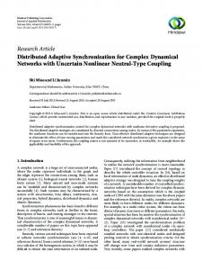
Fig.1 Block diagram of multistep CFAR procedure Fig.1 shows the block diagram of the adaptive CFAR procedure introduced above. Let x1 , x2 , " , xN be the powers in N 0 cells in a reference window and α 0 a threshold coefficient providing a specified false alarm rate

m

.

m

The simplest way to keep the rate of false alarms constant is to make all Pfa( m ) be equal to the updated value of Pfa . Square-law detectors enter a buffer, which stores the cell powers that are simultaneously summed by the cell averager. The result is multiplied by the threshold coefficient, which is obtained from the threshold table for specified N and Pfa . The threshold thus obtained is then compared with each power stored in the buffer. If the

power in the cell under test does not exceed the threshold, the comparator proceeds to the next cell; otherwise, a spike is declared and the detection procedure is initialized. The detection procedure consists of three stages: (1) summation of the spike powers, (2) spike counting and (3) zero insertion (into the buffer instead of the spike power). When all the cell powers in the buffer have passed the comparator the first cycle of the CFAR procedure is completed. If the output of the spike counter is not zero, the next cycle starts by subtracting the sum of the spike powers from the total sum. Then the detection proceeds in the same fashion as that on the first cycle. The only difference is that the number of cells remaining after the spikes rejection determines the threshold coefficient. The procedure is terminated when no spike is detected at the current cycle. As the result of the procedure all targets that are present in the reference window may be detected. Under the condition of Gaussian noise background, the output of square-law detector follows the exponential distribution .As shown in Fig.1, the outputs of the test cell under test, which is the one in the middle of the tapped delay line, is denoted by x0 . The outputs of the cells surrounding the test cell, {xi }, i = 1, 2," , N 0 are combined to yield an estimate z of the noise level in the test cell, that is, z = f ( x1 , x2 ,", xN0 ) (6) Where the operator f denotes the processing of the received observations. The outputs of the cell under test x0 is then compared with the adaptive threshold Tz according to: > X 0 Tz < (7) Where the scaling constant T is selected so that the preassigned probability of false alarm is achieved. Hypothesis H1 denotes the presence of a target in the test cell, while hypothesis H 0 is the null hypothesis. The probability of false alarm may be written as a contour integral 1 −1 (8) PF = − v∫ ω φ X |H (ω )φ X ( −T ω ) 2π i c 0 0

Where λi denotes the parameters of the distribution from which the observation xi is generated. Notice that we use uppercase letters to denote the corresponding observations. The value of λi depends on the contents of the ith cell. If the ith cell contains thermal noise only, λi is normalized to λ0 . If it is immersed in the clutter, λi = λ0 (1 + C ) where C denotes the ratio of average clutter power to thermal noise power at the receiver input. If it is a cell in the homogenous region and it contains a target return then λi = λ0 (1 + Si ) ; Si denotes the ratio of target return average signal power to thermal noise power at the receiver input. However, if it is a cell in the clutter and it contains a target return then λi = λ0 (1 + C + Si ) . Therefore, the MGF of the output of the test cell under hypothesis H0 is given by:

φX0

(11) When the censoring procedure decides that the test cell is in the clear, we censor the higher N − k ordered samples, that is x( k +1) ,", x( N0 ) . The lower k ordered samples are added together to form the estimated of the noise level in the test cell, that is: k

z = ∑ x( i )

(12)

i =1

The MGF of the estimated Z of the noise level in the test cell is obtained [19].

−1  N  k  N − j +1  φ Z (ω ) =   ∏  ω +   k  j =1  k − j +1 

(13)

Thus, the probability of false alarm and detection probability is obtained from (11) and (13) to be:

−1  N  k  N − j +1  PF =   ∏  T +   k  j =1  k − j +1 

 N  k  T N − j +1  Pd =   ∏  +  k  j =1  µ j k − j +1 

contour encloses all the poles of φ X 0 |H0 (ω ) that lie in the

(9)

(10)

PF = φZ [T (1 + C )]

moment-generating function (MGF) of the random variable X . The integration contour c is crossing the real ωaxis at ω1 = c1 and is closed in an infinite semicircle in the left half ω -plane. c1 is chosen so that the integration

f X i ( x ) = (1 λi ) exp ( − x λi )

(ω ) = 1 [1 + ω (1 + C )]

Note that if the test cell is in the homogenous background C = 0 . Consequently, the point at which the integration contour c in (8) is crossing the real ω -axis is such that −1 (1 + c ) < c1 < 0 . Solving the integral in (8), we obtain that

Where φ X ( ω ) = E  exp ( −ω x )  is defined to be the

left half ω -plane. We assume that the cell outputs are observations from statistically independent random variables. That is, the probability density function (PDF) of output of the ith cell is given by

H0

3

(13)

−1 (13)

Distributed CFAR Detector

In this section, the distributed adaptive censored cell-averaging (CCAWCA-CFAR) CFAR detector for a network is defined and appropriate parameters are developed. For a two-sensor network, the equations for the detector in homogeneous background are derived.

Consider the N-sensor distributed network as shown in Fig.2. Here, Yi = {Yij } is observation (excluding the test sample), where i = 1, 2," , N indicates the number of the sensors, and j = 1, 2," , N i , represents the sample number in the range cells available to the ith sensor. In general, Ni1 needs not be equal to Ni 2 . It is assumed that all the sensors scan the same search environment. The sample in the test cell for the ith sensor is denoted by X 0i , In each local CCA-CFAR detector, a few of the largest reference cells are censored and the remaining ones are averaged to estimate the total noise power l =1

Phenom enon H Y 2 ,X 02

Sens or 1 CCA- CFAR S 1 (Z 1 ,X 01 )

Y N ,X 0N

…

Sens or 1 CCA- CFAR

…

…

S 2 (Z 2 ,X 02 )

and

hypothesis

means

no

target,

and

λ1i = λ0i (1 + CNR ) represents the signal-plus-noise power, where SNR is the ratio of signal power to noise. Under H 0 ,

∏ f X ( x0 i | H1 ) H1 0i i =1 > T LR = 2 < L ∏ f X ( x0 i | H 0 ) H 0 0i

Sens or 1 CCA- CFAR S N (Z N ,X 0N )

T

Com parator

i =1

H1  1  1 1  1  > T' − + − X X   01   02 <  λ01 λ11   λ02 λ12  H0

λ01

H1

Fig.2 Distributed CCAWCA CFAR Detector

N

Z = G ( S1 , S 2 , " , S N ) = ∑ Wi X 0 i / Z i . i =1

Fusion center decides the presence or the absence of a target in the test cell by comparing Z with T , where T is an appropriate scaling factor. It is assumed that Yi1 , Yi 2 ," , YiM and YiM +1 ," , YiNi are I.I.D random variables that follow an exponential distribution. In the case of homogeneous noise, E[Yij ] = λ0i , where λ0i is the noise power of the ith sensor. We denote the corresponding density and cumulative distribution function as f ( y ) and F ( y ) , respectively, and let CNR represents the clutter-to-noise power ratio. In the case of nonhomogenrous background, the expected value of Yij is λ0i or λ0i (1 + CNR ) , depending on whether the sample Yij is from noise-only region or from clutter. Assuming a Swerling II fluctuating target, the test sample

(18)

Further simplifying (18) yields

X 01

Then the ratio statistic Si = X 0i Z i from the ith sensor is sent to the fusion center. At the fusion center, the global test statistic Z can be computed by WCA, i.e.

(17)

Where TL is an appropriate threshold. Simplifying (16) gets

Fus i on Cent er U 0 H0

H0

2

G(S 1 , S 2 ,… , S N ) Z

Where hypothesis H1 represents the presence of a target

in clutter background, λ1i equals to λ0i (1 + CNR ) . For convenience and without loss generality, we study performance of the CCAWCA detector in the case of two sensors. At the fusion center, applying a likelihood ratio test (LRT) to the case described by (16) yields

Nim

Z i = ∑ xikl , N im = N i − ji1 − " − jim .

Y 1 ,X 01

x0i , also has an exponential distribution with mean λ1i . The mean λ1i is unknown and depends on the target presence/absence, the clutter level, and the target strength: λ or λ (1+CNR ) under H 0 λ1i =  0i 0i (16)  λ1i＝λ0i (1+ SNR ) under H1

Where w =

H X 02 > 1 +w T λ02 < H0

(19)

λ − λ0i r1 + 1 r , L = 1 ，and ri = 1i r1 + L r2 λ0i Si = X 0 i Z i

Using Si denotes Where Z i =

(20)

Rm

∑x

(21)

ki

k1

From (18) and 19), we get Z = S1 + WS 2 , Since the MGF of the Z i can be represented as [19]

 N i  ki  Ni − ji +1    ∏  s +  ki  ji =1  ki − ji +1 

M Zi ( s ) = 

(22)

Then the probability density function (PDF) of Z i can be denoted as N +1

fZi (zi ) =

− i zi (−1)ki Ni ! ki −1 ki +1 z e , Z>0 (23) i ki !( Ni −ki )!(ki −1)!(ki +1)ki

And the PDF of the test statistic Si at the fusion center is

∞ f Si ( s ) = ∫0 zf ( x0i , zi )dz ∞ = ∫0 zf X 0 i ( sz ) f Zi ( z )dz

F2 = Hypergeometric 2 F1 (24)

−1

( − k 2 ,1 + k1 ;1 − k 2 ;

Substituting (21) and (23) into (24) yields:

 at  s f Si ( s) = + ct  − (1 + ri )  (1 + ri )  Where ati =

, Z>0 (25)

( Ni − ki ) !( ki − 1)!(kii − 1) k

i

, cti =

Pfa = at1at2

ki + 1

Thus, we can evaluate the detection probability of the CCAWCA detector by (26) through (25):

∫∫

S1 +WS 2 >T

f s1 ,s2 ( s1 , s2 )ds1ds2 (27)

Substituting (24) and (25) into (27) yields： at1 s1 −1− k Pd = (− + ct1 ) 1 ∫∫ S1 +WS2 >T (1 + r1 ) (1 + r1 )

× =

at 2 (1 + r1 ) at 1

s2

+ ct 2 )

(1 + r2 )

at 2

(−

∫∫

(1 + r1 ) (1 + r1 ) S1 +WS 2 >T × (−

=

(−

s2 (1 + r2 )

at 1

+ ct 2 )

−1− k2

at 2

µ1 (1 + λ1 ) µ1 (1 + λ1 )

Where: A = A2 = k1k 2 ( A3 = −

−1− k 2

(1 + r1 )

k1 + 1

T

k

W µ2 (1 + λ2 )

µ1 µ2 (1 + λ1 )(1 + λ2 ) k1k 2

(

(28) A1 = A2 + A2 +

N2 + 1 k2 + 1

k

) 2 dy

×

)

−1

)

at 2 (ct1 + at1T ) − at1Wct 2

)(ct 2 + at 2TW

−1 −1− k 2

)

F1 = Hypergeometric 2 F 1 (− k2 ,1 + k1 ;1 − k2 ;

, B1 = B2 + B3

N +1 k T N + 1 k2 B2 = k1k 2 ( 1 ) 1 ( + 2 ) µ2 k 2 + 1 k1 + 1

µ1 µ 2 k1k 2

k

k

{(ct1 ) 1 (ct 2 ) 2 F1

at 2 (ct1 + at1T + at1T ) )(ct 2 + at 2T ) −1−k2 F2 } at 2 (ct1 + at1T ) − at1ct 2

at 1Wc2 (ct 1 + at1T ) + at1Wct 2

)

( −k 2 ,1 + k1 ;1 − k 2 ;

4

−1 − k1

at 2 ( ct1 + at1T + at1TW

µ1µ 2 k1 k 2 ct1 ct 2 k1k 2

( − k 2 ,1 + k1 ;1 − k 2 ;

{(ct1 )k1 (ct 2 ) k2 F1 − (ct 2 + at 2TW −1 ) ×(ct1 + at1T + at1TW

Where: B =

F1 = Hypergeometric 2 F 1

−1− k1

× ( A − A1 )

k

) 1(

ds1ds2

at 1c2 (ct1 + at 2T ) + at1ct 2

)

F2 = Hypergeometric 2 F 1

ct11 ct 22 k1k 2 N1 + 1

S1+WS2 >T

−1−k2

(−s2 + ct2 )

−k −(ct 2 + at 2T )(ct1 + at1T + at1T ) 1

ds1ds2

µ1 µ2 (1 + λ1 )(1 + λ2 ) k

−1−k1

(−s1 + ct1)

(29)

(

+ ct 1 )

∫∫

= at1at 2 × (B − B1)

B3 = −

ds1ds2

s1

( ct1 + at1T ) at 2 + at1Wct 2

.

setting d1 = 1 , d 2 = 1 , W = 1 i.e.：

Ni + 1

Assuming S1 and S 2 are independent each other, the joint PDF between S1 and S2 can be represented as: f S1 , S2 ( s1 , s2 ) = f S1 ( s1 ) f S2 ( s2 ) (26)

Pd = Pr ( S > T ) =

)

We can directly obtain the false alarm probability Pfa by

−1− ki

k

( −1) i N i !

at1W (ct 2 + at 2W T )

F2 }

at1 ( ct 2 + at 2T ) ( ct1 + at 1T ) at 2 + at 1ct 2

)

Numerical Analysis results

In this section, we discuss the performance of the adaptive censored cell-averaging CFAR detector. And we compare its performance with typical detectors such as the central order statistic detector (COS), the OSAND, OSOR, MOS (maximum order statistic) and mOS(minimum order statistic) detector. The specific values of parameters used in our analysis are listed in Table 1. Table1 parameters and calculation values for constant T for Pfa=0.001 T Detector RC k(l) P fa N CCAWCA S1 25 20 0.001 0.0623 S2 25 COS S1 25 20 0.001 41.4120 S2 25 MOS S1 25 20 0.001 10.0508 S2 25 mOS S1 25 20 0.001 52.8443

S2 25 S1 25 20 0.001 34.2625 S2 25 OSAND S1 25 20 0.001 5.5262 S2 25 In Table 1, S1 and S 2 represent sensor 1 and sensor 2, and RCN denotes reference cell number. And we analyze below various ranges of parameters over which the comparisons are made including detector comparisons under homogeneous background clutter and under the interfering target (multi-target) or clutter edge situation. Also we discuss two kinds of situations, in which two sensors have the same SNR/CNR/INR or not. Moreover, since the closed-form expressions for Pd of CCAWCA in nonhomogeneous background is not available, we analyze it using Monte Carlo simulation. Under homogeneous background, the CCAWCA -CFAR outperforms the mOS, OSAND and OSOR detectors, but not as good as the COS detector does. The detection performance of all the CFAR detectors, in the case of homogeneous background and two sensors having the same SNR (i.e. L=1), are shown in Fig.3. When the two sensors have the different SNR, here, we choose the ratio of SNR of sensor 1 to that of sensor 2 is 0.1, and its detection performance are shown Fig.4. In the case of multi-target background, the detection performance are shown in Fig.5-11 (L=1), it analysis the situation is that Pd as a function of SNR when the number of interfering targets at sensor 1 has 2 and sensor 2 varies from 0 to 11. When two sensors have the same SNR (SNR=20, i.e. L=1), the detection performances of all the CFAR detectors are shown in Fig.10. When two sensors have different SNR (i.e. L=0.1), the detection performance is shown Fig.11. From Fig.10 and Fig.11 we can see that all detectors’ performance depend on the selected rank. For number of interfering targets from 0 to 4, the detectors has nearly good performance as the COS detector does. But once the number of interfering targets exceeds its tolerable range, we observed that the mOS, CCAOR, and OSOR perform better than the others, and the other detector have a sharp drop in Pd . OSOR

Fig.4 Pd versus SNR in different weights (L＝0.1)

Fig.5 IR=IL=0

Fig.6 IR=IL=1

Fig.7 IR＝IL=2

Fig.3 Pd versus SNR in different weights L=1)

Fig.8 IR＝IL=3

Fig.9 IR＝IL=4

false alarm probability and detection probability. In summary, the attractive feature of the proposed detector over other CFAR detectors is that it does not need a priori knowledge about the interference in order to perform well. Other CFAR detectors perform well only when the priori information about the interfering environment are appropriately selected. Not enough a priori information will result in severe degradation in false alarm regulation properties or detection performance, especially in acute interfering environments. Without the priori information about the interfering environment or the interference targets not trimming completely, so this algorithm has more CFAR loss. The advantage of the method proposed becomes obvious when dealing with a dense target environment; the algorithm is robust even in the situation where the targets with leakages comprise up to 30% of the reference window. More importantly, the CCAWCA detector holds CFAR characteristic in different SNR case for every sensor.

Acknowledgements Fig.10 Probability of detection versus number of interfering targets at sensor 2(L=1)

This research work was supported by the National Natural Science Foundation of China, No. 60574033 and the 40th National Postdoctoral Science Foundation of China, No. 20060401000.

References [1] Tenney, Robert R., and Sandell, Nils R. Jr. Detection with distributed sensors. IEEE Transactions on Aerospace and Electronic Systems, Vol 17, pp. 501-510, July 1981.

Fig.11 Probability of detection versus number of interfering targets at sensor 2(L=0.1) The numerical analysis results indicate that, in the case of homogeneous background, the performance of the CCAWCA-CFAR detector is not better than that of COS CFAR detectors; but in nonhomogeneous background it performs better than OSAND, OSOR , and COS, while it has a tolerable drop in Pd . And the CCAWCA-CFAR detector requires only half communication band width of the MOS detector’s and the mOS detector’s. The most important advantage of the CCAWCA detector is that it can be available in the csase of different SNR among sensors. In addition, another advantage of the method proposed here becomes obvious when dealing with a dense target environment, because it does not need prior knowledge of the target situation.

5

Summaries and Conclusions

In this paper, we have developed a novel adaptive CCAWCA-CFAR detector used in distributed sensors. For a Swerling II fluctuating target in Gaussian noise of unknown level, we obtain its closed-form expressions of

[2] Sadjadi,E. Hypothesis in a distributed environment. IEEE Transactions on Aerospace and Electronic Systems, Vol 22, pp. 134-137, 1986. [3] Reibman, Amy R. and Nolte, L. W. Optimal detection and performance of distributed sensor systems. IEEE Transactions on Aerospace and Electronic Systems, Vol 23, No. 1, pp. 24-30, 1987. [4] Chair, Z., Varshney, P. K.. Optima data fusion in multiple sensor detection systems. IEEE Transactions on Aerospace and Electronic Systems, Vol 22, No. 1, pp. 98-101, 1986. [5] Hoballah, Imad Y., Varshney, Pramod K.Distributed Bayesian signal detection. IEEE Transactions on Information Theory, Vol 35, No.5, pp. 995-1000, 1989. [6] Hoballah, I.Y., and Varshney, P. K. Neyman-pearson detection using multiple radars. In Proceedings of the 25th IEEE Control and Decision Conference, 1986, pp. 237-241. [7] Srinivasan, R., Distributed radar detection theory. IEE Proceedings, Part F: Communications, Radar and Signal Processing, Vol 133, No. 1, 1986, pp. 55-60.

[8] Thomopoulos, S.C.A., Viswanathan, R.,and Bougoulias, D.K. Optimal distributed decision fusion. IEEE Transactions on Aerospace and Electronic Systems, Vol 25, No.1 5, pp. 761-765, 1989.

[20] Guan Jian, He You, Peng Yingning. Distributed CFAR Detector Based on Local Test Statistic. Signal Processing (Elsevier), Vol 80,No. 2, pp.373～379, 2000.

[9] Eckchain, L.K., and Tenney, R.K. Detection network. In Proceedings of the 21th IEEE Conference on Decision and Control, Dec.1982, pp. 686-691.

[21] Guan Jian, Meng Xiang-Wei, Peng Ying-Ning, He You. The optimality in Neyman-Pearson sense in the distributed CFAR detection with multisensor. Proceedings of the IEEE Radar Conference,2002, 68 – 72.

[10] Eckchian, L.K. Optimal design of distributed detection networks. Ph.D. dissertation, Massachusetts Institute of Technology, Lexington, MA, 1980.

[22] Jing Jiang, Jun Yang, Hong Sun, A Distributed CFAR Detector Based on Local Test Statistics. Journal of Communication and Computer, pp.27 – 31, 2002,

[11] Chair,Z. On Hypothesis testing in distributed sensor networks. Ph.D. dissertation, Syracuse University, NY, Apr.1987.

[23] Guan Jian, He You, Peng Ying-Ning, Meng Xiang-Wei Study of centralized CFAR detection with multisensor, Proceedings of the IEEE Radar Conference, 2001, pp.334 – 337.

[12] Barkat, M., and Varshney, P.K. Decentralized CFAR signal detection. IEEE Transactions on Aerospace and Electronic Systems, Vol 25, pp. 141-149, 1989. [13] Elias-Fuste, A.R., Broquetas-Ibars, A., Antequera, J.P., and Yuste, J.C.M., CFAR data fusion center with inhomogeneous receivers. IEEE Transactions on Aerospace and Electronic systems, Vol 28, No. 1, pp. 276 – 285, Jan. 1992. [14] himonas,S.D., and Barkat,M. A distributed CFAR processor with data fusion for correlated targets in nonhomogeneous clutter. In Proceedings of the IEEE International Radar Conference, 1990, pp. 501-506. [15] .Uner, M. K., and Varshney, P. K. Distributed CFAR detection in homogeneous and nohomogeneous background. IEEE Transactions on Aerospace and Electronic Systems, Vol 32, pp. 84-96, 1996. [16] Amirmehrabi, H., and Viswanathan, R., A new distributed constant false alarm rate detector. IEEE Transactions on Aerospace and Electronic Systems, Vol 33, pp. 85-97, 1997. [17] Uner, M.K., and Varshney, P.K., Decentralized CFAR detection based on order statistics. In Proceedings of the 36th Midwest Symposium on Circuits and Systems, Detroit, MI, 1993, pp. 146-149. [18] Bluiii, R.S., and Kassam, S.A., Distributed cell-averaging CFAR detection of dependent signal returns. In Proceedings of 1993 IEEE International Symposium on Information Theory, 1993, p. 12. [19] Jian Guan; Ying-Ning Peng; You He; Xiang-Wei Meng; Three types of distributed CFAR detection based on local test statistic. IEEE Transaction on Aerospace and Electronic Systems, Vol 38, No. 1, pp. 278 – 288. Jan, 2002.