Distributed Navigation with Unknown Initial Poses ... - Semantic Scholar

Distributed Navigation with Unknown Initial Poses and Data Association via Expectation Maximization Vadim Indelman*, Nathan Michael† , and Frank Dellaert‡ We present a novel approach for multi-robot distributed and incremental inference over variables of interest, such as robot trajectories, considering the initial relative poses between the robots and multi-robot data association are both unknown. Assuming robots share with each other informative observations, this inference problem is formulated within an Expectation-Maximization (EM) optimization, performed by each robot separately, alternating between inference over variables of interest and multi-robot data association. To facilitate this process, a common reference frame between the robots should first be established. We show the latter is coupled with determining multi-robot data association, and therefore concurrently infer both using a separate EM optimization. This optimization is performed by each robot starting from several promising initial solutions, converging to locally-optimal hypotheses regarding data association and reference frame transformation. Choosing the best hypothesis in an incremental problem setting is in particular challenging due to high sensitivity to measurement aliasing and possibly insufficient amount of data. Selecting an incorrect hypothesis introduces outliers and can lead to catastrophic results. To address these challenges we develop a model-selection based approach to choose the most probable hypothesis, while resorting to Chinese Restaurant Process to represent statistical knowledge regarding hypothesis prior probabilities. We evaluate our approach in real-data experiments.

I.

Introduction

Distributed inference is a key capability in multi-robot autonomous systems that is of interest in a variety of problem domains, including surveillance, tracking, localization and mapping. Cooperatively inferring variables of interest, such as robot trajectories, observed objects and tracked targets, results in higher levels of performance, flexibility and robustness to failure. The research community has been addressing different aspects of this problem, considering both centralized and decentralized frameworks. To facilitate cooperative inference it is essential to establish a common reference frame and world model between the robots, so that these can communicate with each other relevant information and correctly interpret it for their needs. While each of these problems has been previously addressed assuming the other problem is solved, only few attempts have been made to solve the two problems simultaneously: determining a common reference frame between the robots, and resolving data association between measurements (e.g. images or laser scans) acquired by different robots. * Faculty of Aerospace Engineering, Technion - Israel Institute of Technology, Haifa 32000, Israel. Part of this research was performed while the author was with the Georgia Institute of Technology. † Robotics Institute, Carnegie Mellon, Pittsburgh, PA 15213, USA. ‡ Institute for Robotics and Intelligent Machines (IRIM), Georgia Institute of Technology, Atlanta, GA 30332, USA.

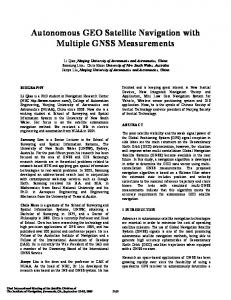
Solving these two coupled problems is important as it will enable the robots, scattered in a complex, previously unknown environment, to establish collaboration without requiring any prior knowledge or infrastructure. For example, starting from some arbitrary guess as to where each robot is and by sharing measurements of onboard sensors, each robot will be capable of inferring the trajectories of other robots in the group, as shown in Figures 1 and 2. 15

5 10

0

5

0

−5 −5

−10 −10

−15

−15

−20

−20 −30

−25

−20

−15

(a)

−10

−5

0

−30

−25

−20

−15

−10

−5

0

5

10

15

(b)

Figure 1: Multi-robot candidate correspondences F r between (a) red and blue, and (b) green and blue robots in the real-world dataset D1. As a common reference frame is not yet established, robot initial poses are set to arbitrary values. Multi-robot data association is a key challenge that shares some similarities with loop closure detection in the single-robot case. Incorrect data association can lead to catastrophic deterioration in performance and should be avoided at all costs; the robotics community has been indeed very active in the last two years in developing robust graph optimization techniques [22, 23, 31, 32] to address this crucial aspect. Multi-robot data association has recently become an active research area as well [9,19,21,26], with the same sensitivity to incorrect correspondences as in the single-robot case. This problem, however, becomes more complicated when the initial relative poses between the robots are unknown. Without a common reference frame, how can the robot decide what information to share with each other? Given the calculated multi-robot constraints based on this shared information, how to determine the inlier correspondences? Addressing this problem requires reasoning about multi-robot data association and initial relative poses concurrently. In this paper we develop a distributed and incremental multi-robot approach that allows a group of robots to simultaneously establish a common reference frame and resolve multi-robot data association on-the-fly. We show that establishing the initial relative pose transformations between different robots is essential to facilitate collaboration between robots: attempting to solve the multi-robot PoseSLAM problem with unknown multirobot data association and unknown initial relative pose transformations leads in all multi-robot correspondences being considered as outliers and therefore rejected. We therefore first infer these transformations and only then address the full multi-robot PoseSLAM problem. Our approach is based on the observation that by analyzing the distribution of multi-

2

2

0

0

0

−2

−2

−2

−4

−4

−4

−6

−6

−6

−8

−8 −5

0 X [m]

5

−8 −5

(a)

0 X [m]

5

−5

(b) −6

−8

−8

−8 Y [m]

−6

−10

−10 −12

−12

−14

−14

−14

−34 −32 −30 −28 −26 −24 −22 X [m]

(d)

−16 −35

−30

X [m]

(e)

5

−10

−12

−16

0 X [m]

(c)

−6

Y [m]

Y [m]

Y [m]

2

Y [m]

Y [m]

robot relative pose constraints it is possible to estimate the transformation between the robot reference frames and identify the inliers in these constraints: we show that this distribution is clustered for inlier and scattered for outlier correspondences, as long as there is no perceptual aliasing. Based on this insight we develop an expectation-maximization (EM) [27] approach to efficiently perform this inference by each of the robots independently, starting from several initial guesses and resulting in different locally-optimal solutions. Choosing the correct solution is a key challenge, as a wrong decision will effectively introduce outliers to the graph optimization. This is particularly true when information is received incrementally, as required for online operation in real autonomous robotic systems: in this case, one needs also to decide whether sufficient amount of information has been received to perform this decision reliably. Furthermore, perceptual aliasing presents additional challenges, as matching observations from different, but similar in appearance environments (such as two corridors) often result in reliable and consistent transformations that erroneously indicate the two environments are the same. These outliers form clusters of their own that compete with the inliers cluster, leading to the problem of choosing the right cluster among several candidates.

−25

−16 −35

−30

X [m]

−25

(f)

Figure 2: Robots’ estimates of each other trajectories expressed in local frame of each robot over time. (a)-(c) Red robot; (d)-(f) Blue robot. Figures (a) and (d) show the identified inlier (black) and outlier (gray) correspondences after a common reference frame has been established. We consider this challenging problem and frame it within a model selection framework [5], developing a probabilistically-sound approach for selecting the most probable cluster. Moreover, we address the question wether there is a correct cluster given the information available to each robot thus far, as the robots might have not observed the

same environment yet. We approach this problem by modeling the prior probability for each cluster using the Chinese restaurant process (e.g., [4,33]) that allows to disambiguate this decision-making as more information is accumulated. Consequently, this paper makes the following contributions: (i) development of a new approach for distributed incremental multi-robot inference with unknown multi-robot data association and initial relative poses; (ii) Model selection for identifying the correct solution among several candidates; (iii) Determining if sufficient information has been obtained to disambiguate potential perceptual aliasing; (iv) Performance evaluation in realistic simulation and in real-world indoor experiments. II.

Related Work

Distributed cooperative localization and multi-robot simultaneous localization and mapping has been extensively studied over the last decade. Many of these research efforts, that can be classified into Full-SLAM (e.g. [11, 15, 16, 30]) and Pose-SLAM (e.g. [3, 17, 18, 20, 30, 34]) approaches, assume the initial relative poses between the robots are known and multi-robot data association has been externally established. Several approaches have been developed to operate also when the initial relative poses between the robots are unknown, still assuming perfect multi-robot data association is given. These approaches, including [1, 6, 35], often use direct relative-pose observations between the robots and assume the identity of the observed robots is known. Relaxing this assumption has been recently investigated in [13]. Multi-robot Pose-SLAM using also indirect relative pose constraints, corresponding to different robots observing the same environment, has been mainly researched under the assumption of perfect data association and an established common reference frame between the robots (e.g. [17, 18, 20, 25]). Determining data association is often treated as a pre-processing separate step from inference over the robot states. Cunningham et al. [9] developed a RANSAC [12] approach for distributed data association, and Montijano et al. [26] compute global correspondences by identifying inconsistent data association in a distributed framework. While these approaches do not require a common reference frame between the robots, they operate within the Full-SLAM paradigm, explicitly performing inference also over the observed structure (e.g. 3D points, objects) in addition to robot states. In contrast, our approach is formulated in Pose-SLAM framework, which has computational advantages over Full-SLAM. Consistency-based outlier rejection has been recently also developed for multi-robot Pose-SLAM [21] assuming direct relative-pose observations, still assuming a common reference frame between different robots is known. To be resilient to outliers overlooked by data association approaches, the robotics community has been recently focusing on robust graph optimization techniques [22, 23, 31, 32]. These new approaches in particular aim to be robust to loop-closures outliers, as current state of the art methods for generating loop closure constraints (e.g. FABMAP place recognition [7]) are not error-free. However, the majority of robust graph optimization approaches are developed for the single robot case, typically not considering the multi-robot case. In a previous recent work [19], we investigated the multi-robot case, considering a centralized and batch setting and without considering perceptual aliasing aspects. An incremental and distributed multi-robot configuration, that is the focus of this paper, has not been investigated thus far to the best of our knowledge.

III.

Problem Formulation and Approach

We consider a group of R robots deployed to collaboratively operate in an unknown environment, initially unaware of each other. Our objective is for each robot r to estimate its own trajectory X r (current and past poses) and additional variables of interest, such as the trajectories of other robots, in a distributed incremental framework. Such a capability is important for multi-robot cooperation in numerous applications; additionally, it allows the robots to extend their sensing horizon and establish a common world model, observed so far by the entire group. Although the latter is not explicitly inferred, it can be always recovered from the estimated poses and sensor observations (see, e.g. [14]). In a centralized problem setting, this problem corresponds to calculating the maximum a posteriori (MAP) estimate Xˆ R = arg max p X R |Z R , XR

(1)

. where R = {1, . . . , R}, and X R and Z R represent the trajectories and the observations of all the robots in the group. We assume the robots share with each other observations of different parts of the environment, which, given data association, can be used to formulate constraints between appropriate poses of different robots. These constraints become part of the underlying graph structure of p X R |Z R and are essential for facilitating collaboration between the robots. Assuming a common reference frame is known, the robots can identify and share with each other only observations of areas that are likely to be observed by other robots. However, in lack of a common reference frame, it is not obvious what information should the robots communicate with each other, as each robot r represents its trajectory X r in its own local frame. Consequently, data association becomes much more challenging because of the high number of outlier correspondences, and as shown in the sequel, is coupled with establishing a common reference frame between the robots. A distributed setting further complicated this problem, as each robot r has only access to Z r 2 Z R , comprising its own observations and observations shared by other robots. Letting X r ✓ X R represent the trajectory of robot r and additional variables of interest, in our case, the appropriate trajectories of other robots (as defined in the sequel), the inference solved by each robot r is Xˆ r = arg max p (X r |Z r ) . Xr

(2)

Below we develop an EM-based approach for solving this problem in an incremental and distributed setting with unknown multi-robot data association and initial relative poses. Since this approach requires the initial relative poses to be first roughly determined, we develop in Section B a method that allows each robot to infer the latter and multi-robot data association simultaneously. As will be seen, the information available to each robot in an incremental problem setting at a given time often supports several possible solutions. The problem then turns into choosing the most probable solution and identifying whether sufficient amount of information has been accumulated to perform this reliably. We show this is particularly important in the incremental setting in the presence of measurement aliasing. In Section V we address this crucial step, formulating the problem within a model-based selection paradigm.

IV.

Incremental Distributed Framework

In this section we develop a Bayesian formulation for the inference problem (2) to be solved by each robot r. First, however, we discuss our approach for information sharing between different robots, when a common reference frame is unknown. Throughout the paper we use the notation xri 2 X r to represent the pose of robot r at time ti , expressed in its local reference frame. We assume each robot r shares at each time tk its current measurement zkr , if it is informative, and also tracks all these informative measurements {zir } over time. Additionally, it shares its current pose estimate xˆrk and local measurements from its onboard sensors. We assume these measurements and information are shared at some basic frequency, or upon moving sufficient distance (for example, 0.5 meters in our implementation). Sharing only local measurements guarantees consistent multi-robot estimates [8] (additional approaches include [2, 18]). While this may seem as a lot of information to share, in practice one can represent all these measurements by a single relative pose constraint with an appropriate covariance (see e.g. [8]). 0 Any robot r that receives a measurement zkr from some robot r0 , generates candidate 0 correspondences by matching zkr with its own informative measurements {zir }. Each such 0 0 successful match urk,l,r between zkr and zlr 2 {zir } represents a (relative-pose) constraint 0 involving the poses xrk and xrl , with l  k . We denote by F r the set of multi-robot data association, that is available to robot r, where each individual data association r 0 ,r 0 r (r , k, l) 2 F represents the constraint uk,l . An examples of the multi-robot candidate correspondences set F r is shown in Figure 1. The figure illustrates the candidate correspondences in F r between the blue robot and other robots (green and red). Since the initial relative poses between the robots are unknown, these transformations were set to arbitrary values, i.e. the initial pose of each robot was chosen arbitrarily. Observe that many of these correspondences in F r are outliers. One may argue that outliers can be directly identified and rejected by matching algorithms, such as RANSACbased fundamental matrix estimation in the case of image observations or ICP matching in the case of laser measurements. However, this argument is only partially true: while these algorithms are capable of accurate relative pose estimation given observations of a common scene, identifying the fact that two given observations were acquired from different parts of the environment is a much more challenging task. In the single robot case, a related aspect is establishing loop closures; also here current techniques cannot guarantee outlier-free data associations and approaches for robust graph optimization are actively investigated in recent years. Similarly, in the multi-robot framework that we consider herein, multi-robot data association cannot be assumed outlier-free. Moreover, perceptual aliasing will often result in numerous false data associations. In particular, when fed with two laser scans from different yet similar parts of the environment (e.g. corridors, hallways), ICP will typically produce some relative pose estimate, with a reasonable uncertainty covariance and number of matched points between the two scans. Not only this estimate is completely wrong, but also similar erroneous estimates will be obtained for all such outliers, making it difficult to identify these are all outliers. We address this crucial aspect in detail in Section V. We can now formulate the joint probability distribution (2) given all the measurements

available to robot r:

⇣ ⌘ . R\{r} p (X r |Z r ) = p X r , X R\{r} |Z r , Z R\{r} , Zlocal ,

(3)

0

where the set X R\{r} represents all the poses xri of robots r0 2 R that contributed at least one correspondence to F r . Accordingly, Z R\{r} represents the actual measurements R\{r} that participate in those constraints, and Zlocal the local observations of these robots, both shared by these robots. For brevity, we collect all these measurements into the set Z r and also let X r represent all the random variables in Eq. (3): . . R\{r} Z r = Z r [ Z R\{r} [ Zlocal , X r = X r [ X R\{r} . (4) 0

Given the multi-robot data association F r , and the appropriate constraints urk,l,r , the joint pdf (3) can be expressed as ⇣ ⌘ Y ⇣ 0 ⌘ R\{r} r ,r r 0 r r r r R\{r} r p (X |Z ) / p (X |Z ) p X |Zlocal p uk,l |xk , xl (5) (r 0 ,k,l)2F r

where p (X r |Z r ) is only a function of local observations Z r . Since we assume no a priori knowledge about the environment and the initial pose of the robots, the reference frame of each robot is set arbitrarily an value. As the robots express their local trajectories with respect to different reference systems, the measurement likelihood term in Eq. (5) is ✓ ⇣ 0 ⌘ ⇣ 0 ⌘ 2◆ 1 r ,r r 0 r ,r r r0 r p uk,l |xk , xl / exp err uk,l , xk , xl , (6) 2 ⌃ with

and

⇣ 0 ⌘ 0 . 0 err urk,l,r , xrk , xrl = urk,l,r ⇣ 0 ⌘ . 0 h xrk , xrl = xrk

⇣

⇣ 0 ⌘ h xrk , xrl , Trr

0

⌘ xrl ,

(7) (8)

where we use the notation in a b to express b locally in the frame of a, and to represent the compose operator [24]. 0 In Eq. (8), Trr represents a transformation between the reference frames of robots r and r0 . Observe that if this transformation was known, performing inference over Eq. (5) while identifying and rejecting outliers could be addressed by robust graph optimization techniques [22,23,31,32]. In contrast, we consider multi-robot data association and initial relative poses are both unknown. A.

Multi-Robot Data Association and Localization via EM

Instead of 0assuming multi-robot data association is given, we introduce a latent binary r ,r variable jk,l for each correspondence (r0 , k, l) 2 F r and use the convention that this r 0 ,r r0 ,r correspondence is an inlier if jk,l = inlier and accordingly outlier when jk,l = outlier. Denoting all the latent variables representing data association between robot r and other robots by J r and considering it to be part of the inference, the probabilistic formulation (5) turns into: ⇣ ⌘ Y ⇣ 0 ⌘ ⇣ 0 ⌘ 0 R\{r} r ,r r,r 0 p (X r , J r |Z r ) / p (X r |Z r ) p X R\{r} |Zlocal p jk,l p urk,l,r |xrk , xrl , jk,l . (9) (r 0 ,k,l)2F r

We let ⌃in and ⌃out to represent the covariances corresponding ⇣to inlier and outlier ⌘ 0 r 0 ,r r 0 r r,r distributions, respectively, with ⌃in ⌧ ⌃out . The probability p uk,l |xk , xl , jk,l in 0

0

r,r r,r Eq. (9) can be evaluated, for both jk,l = inlier and jk,l = outlier, using Eq. (6). r0 Assuming for the moment the initial relative poses Tr are known, we can jointly infer the robot trajectories and multi-robot data association via Eq. (9). In particular, the MAP estimate over robot states is given by X Xˆ r = arg max p (X r |Z r ) = arg max p (X r , J r |Z r ) . (10) Xr

Xr

Jr

However, since the above optimization is computationally expensive, we resort to an Expectation-Maximization approach, a single iteration of which can be formulated as ˆ ⇣ ⌘ h ⇣ ⌘i r r r ˆ X(i+1) = arg max p J r |Xˆ(i) , Z r log p X r |Jˆ(i) , Z r dJ r , (11) Xr

where the notation (i) represents an iteration number. 0 We note that when the initial relative pose Trr between any two robots r and r0 is unknown, performing inference over Eqs. (11) or (9) is doomed to fail: since the 0 transformation Trr is unknown and can only be arbitrarily set, each candidate multi0 robot data association (r0 , k, l) 2 F r with a corresponding constraint urk,l,r will typically 0 0 result in high discrepancy between urk,l,r and the prediction h xrk , xrl from Eq. (8), i.e. ⇣ 0 ⌘ 0 high errors err urk,l,r , xrk , xrl . These high errors will be obtained both for inlier and outlier correspondences. ⇣ 0 ⌘ 0 r ,r r 0 r 0 ,r r r ,r Since ⌃in ⌧ ⌃out , the probability p uk,l |xk , xl , jk,l will be higher for jk,l = outlier 0

r ,r than jk,l = inlier, regardless if the correspondence (r0 , k, l) 2 F r is an inlier or outlier in practice. As a result, attempting to infer both multi-robot data association and robot trajectories will lead to all candidate correspondences in F r to be identified as outliers. It is for this reason that initial relative poses must be first estimated so that the error in Eq. (7) could be used to distinguish between inlier and outlier correspondences. This observation is illustrated in Figure 3 for the candidate correspondences between the blue and red robots shown in Figure 1a. The figure summarizes the errors (7) for all such correspondences evaluated using ground truth value for the initial relative pose 0 0 transformation Trr (Figure 3a) and the inferred transformation Tˆrr at each time step. For each case, the errors are separately shown for inlier and outlier correspondences, determined from ground truth data - the filled areas represent the minimum and maximum 0 of these errors. As seen, when using the true transformation Trr , the errors substantially differ for inliers and outliers, and therefore they can be distinguished from each other. On the other hand, as evaluating Eq. (7) using the arbitrarily chosen robot reference frames, results in high errors and, more importantly, the inlier and outlier error levels overlap each other and therefore the inlier and outliers cannot be easily distinguished. Only after this transformation is correctly established, the errors drop and a natural segmentation into inliers and outliers arises (right area in Figure 3b). 0 Consequently, we propose first to infer the transformations Trr and only then we proceed to infer robot trajectories via the EM optimization (11). In the following sections 0 we describe our approach for estimating the transformations Trr without assuming multirobot data association is given.

14

10 8 6 4 2 0 0

Inlier errors Outlier errors

35 Translaiton error norm [m]

Translaiton error norm [m]

12

40 Inlier errors Outlier errors

30 25 20 15 10 5

50

100 150 Pose index

(a) Ground truth Trr

200 0

250

0 0

50

100 150 Pose index

(b) Inferred Trr

200

250

0

Figure 3: Distribution of inlier and outlier correspondences error over time evaluated 0 using (a) ground truth and (b) inferred initial relative pose transformation Trr . The shown filled areas represent the maximum and minimum norm of translation error in the actual inlier and outlier correspondences as determined from ground truth data. Using 0 ground truth Trr (a) the inliers can be easily distinguished from outliers. In contrast, 0 (b) shows that for arbitrary value of Trr the errors for inlier and outlier correspondences 0 overlap, and only after estimating the transformation Trr (around pose index 140), inliers and outliers become distinguishable. B.

Distributed Inference over Initial Relative Pose via EM

Our approach is based on the following key observation: given local robot trajectories, each candidate multi-robot correspondence (r0 , k, l) 2 F r , regardless if it is inlier or 0 outlier, suggests a solution for the transformation Trr . However, only the inlier correspondences will produce similar transformations, while those calculated from outlier correspondences will typically disagree amongst each other, unless these outliers are caused by measurement aliasing. We illustrate this concept in a synthetic toy example in Figure 4. Ground truth robot trajectories are given in Figure 4a; candidate matches between two of the robots (red and blue) are shown in Figure 4b, with robot initial poses set to arbitrary values. Many of these correspondences are outliers - in this simple example we assume there is 0 no measurement aliasing. The distribution of the transformation Trr , calculated for each correspondence, is shown in Figure 4c. One can clearly observe the cluster corresponding to the correct transformation. Real-world scenarios, however, often exhibit some level of measurement aliasing, which often leads to multiple clusters and further complicate the identification of the correct 0 transformation Trr . Examples are given throughout the paper (e.g. Figures 9 and 10); our approach addresses this challenge as we discuss in the sequel (Section V). Based on the above key observation, we now formulate an EM-based optimization that allows each robot to recover the initial relative pose with other robots (i.e. establish a common reference frame) in a distributed manner. The MAP estimate of an initial relative pose between robot r and each robot r0 2

60

Robot 1 Robot 2 Robot 3

10 5

60

40

−5

20

30

Y [m]

Y [m]

0 Y [m]

40

50

20

0

−10

−20

10 −15

0

−20

−10

−40

−5

0

5

10

15 X [m]

20

25

30

35

−20

0

(a)

20 X [m]

40

60

(b)

−60 −60

−40

−20

0 X [m]

20

40

60

(c)

Figure 4: Synthetic toy example illustrating proposed concept without considering perceptual aliasing aspects. (a) ground truth trajectories for three robots; (b) candidate matches between blue and red robots. Robot initial poses are unknown and set to ar0 bitrary values. (c) Distribution of the transformation Trr between blue and red robots, calculated for each candidate match shown in (b). Planar case is considered (x, y axes correspond to position, arrow direction to orientation). The cluster corresponds to inliers and to correct transformation. R \ {r} can be written as

⇣ 0 ⌘ 0 Tˆrr = arg max p Trr |Xˆ r , Z r , Trr0

(12)

where, Xˆ r and Z r are defined in Eq. (4). This inference can be solved by each robot r in a distributed fashion, based on the available observations Z r . Similar to Eq. (10), we introduce the latent variables J r to this inference problem ⌘ X ⇣ 0 r0 r r ˆr r ˆ Tr = arg max p Tr , J |X , Z , (13) Trr0

Jr

and re-write the above equation in EM framework: ˆ ⇣ ⌘ h ⇣ 0 ⌘i 0 r0 ˆ Tr = arg max p J r |Tˆrr , Xˆ r , Z r log p Trr |Jˆr , Xˆ r , Z r dJ r , Trr0

(14)

where the iteration number was omitted (see Eq. (11)). The underlying EM equations for Eq. (14) are given in the Appendix. Solving Eq. (14) involves a non-linear optimization that converges to a local minima given an initial guess for a solution. As the optimization problem (14) is highly nonconvex, an initial solution in the vicinity of the global minima is required to guarantee 0 convergence to the correct transformation Trr . How to obtain such an initial solution? We recall the key observation from the beginning of this section and using the available robot local trajectories Xˆ r we calculate 0 an initial relative pose for each correspondence (r0 , k, l) 2 F r resulting in a set Trr (F r ). We then analyze the distribution of this set and perform a very naïve clustering for each 0 element in Trr separately: we simply choose k most common values that are sufficiently far away from each other. We use k = 5 and consider two entries to be sufficiently apart if the difference is above the corresponding std in ⌃in : 0.5 meters for position and 0.05 radians for rotation. Instead of considering all the possible combinations for each axis as

0

initial solution, i.e. k n where n is the dimensionally of Trr , we discard any entries that 0 do not have a nearby initial relative pose in Trr (F r ). 0 This procedure generates several initial solutions for Trr ; running the EM optimization 0 (14) on each one of these solutions produces locally-optimal initial relative poses Tˆrr . We 0 merge different hypotheses that converge to the same value Tˆrr . Each of these estimates is optimal given the corresponding partitioning of the multi-robot data association Jˆr into inliers I and outliers O, as calculated in the E step in EM, see Eq. (14). . We shall now use the term hypothesis h = {I, O}, with I [ O = J r , to represent each such partition and collect all these hypotheses into the set H. Note that each hypothesis 0 h 2 H leads to an estimate of Trr according to ⇣ 0 ⌘ 0 Tˆrr (h) = arg max p Trr |h, Xˆ r , Z r . (15) Trr0

Figure 9b illustrates the distribution of relative pose constraints for each correspondence (r0 , k, l) 2 F r (planar case is considered: x and y axes correspond to position, arrow 0 direction represents orientation). The transformations Tˆrr (h) for each hypothesis h 2 H are denoted by red bold arrows. As there are often more than one hypothesis in H, one has to choose which hypothesis 0 0 ⇤ h 2 H to use and set the initial relative pose to Tˆrr = Tˆrr (h⇤ ) to be later used in the underlying optimization of Eq. (11). Recalling the discussion from Section A, identifying the correct hypothesis in H is crucial, especially in the presence of perceptual aliasing. In the next section we develop a probabilistic method for choosing the most probable hypothesis, focusing in particular on the complexities introduced by the incremental framework that is essential for online operation. V.

Hypothesis Model-Based Selection

In this section we develop a probabilistic approach for choosing the most likely hypothesis, given the current information from the set H. An incremental setting, in which information (i.e. robot trajectories, local observations and multi-robot correspondences) is obtained gradually, introduces a number of challenges. How to know sufficient amount of information has been accumulated to reliably estimate the initial relative poses? For example, robot trajectories and observed environments may initially not overlap (or not overlap at all), in which case all multi-robot correspondences are outliers. Measurement aliasing, i.e. observations of similar but different environments complicate the problem even further: consider the robots start operating in two nearby somewhat similar environments (e.g., corridors). Each robot r shares informative measurements, as described in Section IV, match measurements transmitted from other robots against its own informative measurements and introduces the matches as candidate correspondences into the set F r . Since the two environments are similar but different, not only these matches will be outliers, but they will also be consistent with each other, i.e. suggesting the two environments are actually the same. This translates directly into a hypothesis h = {I, O} with many inliers, all of which are actually (consistent) outliers. Figure 10b shows such a case in a real-world scenario: the robots travel in two different corridors, however because these corridors are similar in appearance many consistent matches between scans from the two corridors are generated, leading to the cluster emphasized by red ellipse). Note that even after the robots observe some areas in common, the correct hypothesis

(corresponding to true inliers) will have to compete with the consistent-outlier hypothesis. Making a wrong decision and choosing an incorrect hypothesis will lead to catastrophic results as outliers will be introduced into the multi-robot optimization (11). This is demonstrated Section VI-C (Figure 10), where as the result of choosing the wrong cluster (denoted by red ellipse), robot trajectories are incorrectly aligned (ground truth trajectories are shown in Figure 8a) and all the true inlier correspondences are considered as outliers. We approach this challenging problem within a model selection framework, aiming to ⇣ ⌘ r r ˆ calculate the probability of each hypothesis h in the set H: p h|X , Z . This probability can be obtained by integrating over all possible values of the continuous random variable 0 Trr : ⇣ ⌘ ˆ ⇣ 0 ⌘ r r ˆ p h|X , Z = p T r , h|Xˆ r , Z r (16) r

Tr21

Applying Bayes rule one can write ⇣ ⌘ ˆ r r p h|Xˆ , Z =

r

Tr21

r

⇣ ⌘ ⇣ 0 ⌘ c · p Z r |Trr21 , h, Xˆ r p Trr , h|Xˆ r

(17)

⇣ ⌘ . with a hypothesis-independent constant c = 1/p Z r |Xˆ r that needs not be calculated. Factorizing the last term as ⇣ 0 ⌘ ⇣ 0 ⌘ ⇣ ⌘ p Trr , h|Xˆ r = p Trr |h, Xˆ r p h|Xˆ r , (18) Eq. (17) turns into

with

⇣

⇣

⌘ ⇣ ⌘ ⇣ ⌘ r r r r ˆ ˆ ˆ p h|Z , X = c · p h|X p Z |h, X ,

(19)

r

⌘ ˆ r ˆ p Z |h, X = r

Trr0

p

⇣

0 Trr |h, Xˆ r

⌘ ⇣ ⌘ r r0 r ˆ p Z |Tr , h, X .

(20)

To calculate hypothesis probability needs to be ⇣ (17), ⌘ each of the terms in Eqs. (19)-(20) ⇣ ⌘ 0 r evaluated: the hypothesis prior p h|Xˆ , relative-pose transformation prior p Trr |h, Xˆ r , ⇣ ⌘ 0 and the measurement likelihood term p Z r |Trr , h, Xˆ r . We proceed by first discussing the measurement likelihood term. Recalling the hypothesis definition, h = {I, O}, and writing down individual inlier and outlier observation terms we get ✓ ⇣ ⌘ ⇣ ⌘ 2 ◆ Y 1 0 r r0 r r r p Z |Tr , h, Xˆ = k (h) exp err ui , Xˆ , Tr · 2 ⌃in i2I ✓ ⇣ ⌘ 2 ◆ Y 1 r r0 ˆ exp err uo , X , Tr , (21) 2 ⌃out o2O 0

where we used ui and uo to represent the appropriate relative pose constraints urk,l,r and err (.) is defined in Eq. (7). The hypothesis-dependent coefficient k (h) is defined as Y 1 1 . Y p p k (h) = . |2⇡⌃in | o2O |2⇡⌃out | i2I

(22)

⇣ ⌘ 0 Considering p Trr |h, Xˆ r can be expressed as the Gaussian p

⇣

0 Trr |h, Xˆ r

⌘

= N (T0 , ⌃0 ) .

(23) 0

with known parameters T0 and ⌃0 (as discussed in Section B), the integrant q Trr in Eq. (20), ⇣ 0⌘ ⇣ 0 ⌘ ⇣ ⌘ 0 . q Trr = p Trr |h, Xˆ r p Z|Trr , h, Xˆ r , (24) can be expressed using Eqs. (21)-(22) and (23). Since the involved distributions are all Gaussians, we can represent this expression by a single Gaussian ⇣ 0⌘ ⇣ 0 ⌘ q Trr = N Tˆrr , ⌃M AP , (25) 0 0 where the MAP estimate is obtained by Tˆrr = arg maxTrr0 q Trr , and can be then used as a linearization point to calculate the covariance ⌃M AP . Recall the relation ˆ p a exp kx xˆk2⌃M AP = a |2⇡⌃M AP |, (26)

x

where the notations xˆ and ⌃M AP represent, respectively, the MAP estimate and covariance of some random variable x. Substituting Eqs. (24)-(25) back to Eq. (19) and using the above relation we get the following expression for the hypothesis probability: ⇣ ⌘ ⇣ ⌘ p p h|Z r , Xˆ r = c · p h|Xˆ r k 0 (h) |2⇡⌃M AP |, (27) . where k 0 (h) = k (h) · p

1 . |2⇡⌃0 |

⌘ ⇣ ⌘ r r0 r ˆ ˆ The remaining missing parts are the priors p h|X and p Tr |h, X . We now discuss each of these terms, and then elaborate on our approach for selecting the most likely hypothesis h⇤ 2 H, given the calculated hypotheses probabilities. A.

⇣ ⌘ Hypothesis Prior p h|Xˆ r

⇣

Hypothesis prior is an important component in deciding which hypothesis to choose from ⇣ ⌘ r r0 r the set H. While the measurement likelihood p Z |Tr , h, Xˆ essentially prioritizes hypotheses with higher number of inliers (since Rin ⌧ Rout , see Eq. (22)), it does not address the question whether sufficient amount of information has been accumulated to make a decision. In other words, given a set H there is always a hypothesis with the highest measurement likelihood (i.e. highest number of inliers); how to decide if that hypothesis is unambiguous and should be indeed chosen? This aspect is particularly crucial in the incremental setting in the context of measurement aliasing that can lead to a dominant hypothesis of consistent outliers (see Section V): Note that each correspondence, regardless if it is considered inlier or outlier by a hypothesis, is the result of a high-quality match between two observations - in our case, ICP match between two laser scans. Therefore, the main reason for a correspondence to be an outlier in practice, i.e. highly-confident match between two scans from different

areas, is perceptual aliasing. Relying only on the measurement likelihood term, it is easy to mistakenly choose this incorrect hypothesis. ⇣ ⌘ To address this crucial issue we argue the hypothesis prior, p h|Xˆ r , can provide insight as to how likely is the hypothesis h = {I, O} is in the first place. Given the robot local trajectories, one can reason about the partitioning of the set F r into inlier and outlier sets I and O, respectively, even without the actual measurements of the corresponding constraints. Additionally, we introduce into an additional hypothesis h0 = {I0 , O0 } into the set H: this hypothesis, that we denote as the null-hypothesis, corresponds to perceptual aliasing, i.e. it represents the possibility that all of the correspondences are actually outliers (I0 ⌘ ). The prior probabilities all hypotheses in H, including the null-hypothesis h0 , can now be calculated as⌘we describe next. The most likely hypothesis h, according⇣ to the ⇣ ⌘ r ˆ posterior p h|X , Z r from Eq. (27) is then chosen only if its prior probability p h|Xˆ r is significantly dominant compared to all other hypotheses in H. That way we wait until sufficient information is accumulated to disambiguate which hypothesis is the correct one. The underlying basic assumption in our approach is that since the robots are operating in closed indoor environments, they will eventually observe common places. Each given candidate correspondence can therefore represent the same place, observed by two different robots, or two different places. However, the number of unique places is unknown ahead of time. To capture this probabilistically, we resort to the Chinese restaurant process (and the closely related Dirichlet process), see e.g. [4, 33], which has been recently used for topological mapping [29]. Next, we provide a brief overview of the Chinese restaurant process (Section V-A.1), and then in Section V-A.2 describe the details of our approach. 1. Chinese Restaurant Process According to the Chinese Restaurant Process, the probability of observing a new place, after previously observing n unique places, is given by ↵ ↵+n

1

(28)

,

where ↵ is a concentration parameter. This parameter defines the extent in which repeated observations of the same place take place - larger ↵ corresponds to higher probability of observing a new place; see Figure 5a that describes the evolution of the probability in Eq. (28) as a function of n and ↵. One can observe from the figure and from Eq. (28) that this probability decreases with n for a given ↵. Based on Eq. (28), it is straightforward to show [29] that, given n observations, the probability of observing n unique places can be written as: ↵n j=1 (↵ + j

. f (n) = Qn

1)

.

(29)

Figure 5b illustrates this probability as a function of n and for different values of ↵. As seen, this probability decreases with n for a given ↵, corresponding to our above assumption that observing only new places becomes less likely as we make more observations.

1 0.9

0.8

0.8

0.7

0.7

0.6

0.6

0.5

Probability

Probability

1 0.9

α=10 α=100 α=300 α=500 α=1000 α=10000

0.4 0.3 0.2

0.4 0.3 0.2

0.1 0 0

α=10 α=100 α=300 α=500 α=1000 α=10000

0.5

0.1 20

40 60 Number of distinct places

(a)

80

100

0 0

20

40 60 Number of distinct places

80

100

(b)

Figure 5: Chinese restaurant process: (a) probability of observing a new place and (b) probability of observing n unique places for different values of ↵. See text for more details. 2. Hypothesis Prior Calculation via Chinese Restaurant Process We will now make use of the above model (29) and develop an approach for quantifying the hypothesis prior for each h 2 H. Our approach is based on the following interpretation of inlier and outlier correspondences, as determined by a given hypothesis h = {I, O} 2 H: an inlier i 2 I relating two different poses of robots r and r0 indicates the two poses are close to each other (generating overlapping observations); accordingly, the involved two poses in an outlier correspondence o 2 O are considered as two different, unique, places. More formally, we let min and mout represent, respectively, the number of inliers and outliers in a given hypothesis h = {I, O} 2 H and denote by m the overall number of candidate correspondences. Note that m is the same for all hypotheses in H, and also m = min + mout . Given some hypothesis h = {I, O} 2 H, we approximately capture the number of unique places due to inlier correspondences as min , i.e.: each inlier correspondence is modeled to contribute a single unique place: as mentioned in Section IV, a new informative measurement is shared by each robot r only if it has moved certain distance since it shared the previous informative measurement. Therefore any two inlier correspondences i1 , i2 2 I, even they involve sequentially shared measurements, will contain some unique information regarding the environment (since the robot moves between one shared measurement to another). Moreover, only a small portion of the measurements pairs (originating from different robots) are successfully matched and added as candidate correspondences. Consequently, the number of unique observed places due to inlier correspondences is modeled as min . Similarly, we consider any two pairs of outlier correspondences o1 , o2 2 O to represent four different places, and thus approximately capture the number of unique observed places due to outliers as 2mout . We make yet another approximation at this point, and consider the unique places contributed by inliers and outliers do not overlap. Based on the above, we model the number of unique places for each given hypothesis as

n (h) = 2mout (h) + min (h) ,

(30)

where the parameters mout and min are hypothesis-specific. We leave the investigation of methods to relax the above assumptions and capturing more accurately the number of unique places for each hypothesis to future work. Observe that while the number of involved pairs of cells, m, is the same for all hypotheses in H, the number of unique places, n, changes from one hypothesis to another in the range n 2 [m, 2m]. In particular, n always assumes the highest value for the nullhypothesis (mout = m, min = 0) and, on the other extreme, the lowest value for all-inliers hypothesis (mout = 0, min = if such a hypothesis exists in H. ⇣ m), ⌘ r ˆ The prior probability p h|X of each hypothesis h 2 H can now be calculated from Eq. (29) using the hypothesis-specific value for n that is calculated according to Eq. (30). We further normalize the prior probabilities of all hypotheses in H by . X ⌘= f (n (h)) (31) h2H

to obtain a valid probability distribution: ⇣ ⌘ f (n (h)) p h|Xˆ r = . ⌘

(32)

The above provides a mechanism to decide if sufficient information has been accumulated to indicate a certain hypothesis is dominant with respect to competing hypotheses while explicitly accounting for potential measurement aliasing via the introduction of the nullhypothesis. In particular, for a given m and ↵, hypotheses with many inliers span different parts of robot trajectories. These hypotheses get higher probabilities since the number of unique places n is smaller for such hypotheses: the two extreme cases are hypotheses with only inlier or only outlier correspondences, corresponding, respectively, to n = m and n = 2m. In general, the parameter n for some hypothesis is given by m, with 1   2. One can verify from Eq. (29) that f ( m) decreases with (see also Figure 5b). The intuition here is that, at each given time (i.e. fixed m), a hypothesis whose inliers involve larger portions of robot trajectories (smaller n) is less prone to measurement aliasing over a hypothesis whose inliers only involve a small area (larger n). How one determines if sufficient information has been obtained so that a decision regarding the most probable hypotheses can be made? To address this question we recall the Chinese restaurant model (29) and formulate the following lemma. Lemma. The ratio between hypotheses prior probabilities increases as more information is accumulated, i.e. as more unique places are observed (n increases). Proof. We consider any two different hypotheses hi , hj 2 H and denote the number of unique places in these hypotheses by ni and nj , with ni , nj 2 [m, 2m]. Without losing ⇣ ⌘ generality, we assume ni < nj and therefore from the discussion above: p hi |Xˆ r > ⇣ ⌘ p hj |Xˆ r . Since both probabilities are calculated using the same normalization constant ⌘ (Eq. (31)): f (ni ) > f (nj ).

Now, we can always find parameter 2 [1, 2], such that nj = ni and therefore express the ratio f (ni ) /f (nj ) ⌘ f (ni ) /f ( ni ) via Eq. (29) as follows: ↵ ni j=1 (↵ + j

. f (ni ) /f ( ni ) = Qni

1) =

·

Q

ni j=1

1 ↵(

1)ni

(↵ + j ↵ ni ni Y

1)

(↵ + j

= 1) =

j=ni +1

1 ↵(

(↵ + ni 1)! . 1)ni (↵ + ni )!

Since 2 [1, 2] and ↵ > 1, the above expression monotonically increases with ni , as shown in Figure 6. However, increasing ni corresponds to accumulating more information, i.e. adding new candidate correspondences to the set F. Therefore, with time, the prior for any two given hypotheses becomes more distinguishable. The implication of the above Lemma is that, as more information is accumulated, it becomes possible to disambiguate between the different hypotheses. The parameter ↵ determines how fast this process is, and therefore this parameter can be considered as tuning parameter to be set according to prior knowledge regarding the environment expected size, if such knowledge exists. In particular, too small value of ↵ will lead to premature down-weighting of the null hypothesis, thereby increasing sensitivity to measurement aliasing. On the other hand, larger values of ↵ will require accumulating more information before the prior of the appropriate hypothesis becomes sufficiently dominant to facilitate reliable decision. In ⇣ our ⌘current implementation, we wait until the (normalized) prior of a hypothesis is p h|Xˆ r 0.8 before considering sufficient data exists to make a decision. The final ⇣ ⌘ decision is of course made based on the overall hypothesis probability p h|Xˆ r , Z r , as described in Section V. 1.5 β=1.2

β=1.4

β=1.6

β=1.8

β=2

Probability ratio

0.1 1

0.08 0.06 0.04 0.02

0.5

0 0

0

5

5

10

15

20

10 Number of distinct places

15

20

Figure 6: Probability ratio f (n) /f ( n) with 1 

 2.

This concept is illustrated in a toy example in Figure 7 that considers 3 different hypotheses that are detailed in Table 1: the null hypothesis (h0 ), hypothesis with half of the correspondences inliers (h1 ), and hypothesis with only inliers (h2 ). The figure shows the evolution of the hypotheses prior as a function of m. One can clearly observe that the prior probability of the null-hypothesis decreases as m increases, and the prior for h2 (all

1

1

0.8

0.8

0.8

0.6 0.4 0.2 0

Probability

1

Probability

Probability

inliers) gradually increases. The gap between the latter and the other two hypotheses (h0 and h1 ) drastically increases as well, corresponding to higher confidence level in choosing h2 as a valid hypothesis candidate.

0.6 0.4 0.2

h0

h1 Hypotheses

h2

0

(a) m = 5

0.6 0.4 0.2

h0

h1 Hypotheses

h2

0

h0

(b) m = 10

h1 Hypotheses

h2

(c) m = 20

Figure 7: Prior probabilities of 3 different hypotheses h0 , h1 and h2 (see Table 1) as a function of m. Larger m corresponds to accumulation of additional information. Parameter ↵ is set to 50 in all cases. h

Description

min

mout

n

h0 h1 h2

null-hypothesis half inliers, half outliers all inliers

0 0.5m m

m 0, 5m 0

2m 1.5m m

Table 1: Considered three different hypotheses in toy example from Figure 7. See text for more details.

B.

⇣ ⌘ 0 Initial Relative Pose Prior p Trr |h, Xˆ r

Given the inlier and outlier correspondences in F r but without the actual measurements, our ability to say anything ⇣ informative ⌘ regarding the prior on the initial relative pose r0 r between the two robots, p Tr |h, Xˆ , is very limited. 0

Although, in principle, one could consider about what values of Trr are unreasonable, we currently employ a basic approach: We assume that because of the way 0constraints are generated (see Section IV), on average, the relative-pose measurements urk,l,r are zerobiased and therefore consider each measurement likelihood term to be distributed according to N (0, ⌃high ) where ⌃high is a high uncertainty covariance (we ⇣ ⌘ use 10 meters in r0 r ˆ position and 90 degrees in rotation). We therefore model p Tr |h, X as the Gaussian: ⇣ 0 ⌘ p Trr |h, Xˆ r =

C.

Y

. N (0, ⌃high ) = N (T0 , ⌃0 ) .

(r 0 ,k,l)2F r

Choosing the Most Probable Hypothesis

Decision on the most probable hypothesis is made as follows. We calculate the probabilities Eq. (27) of only the most promising hypotheses, identified by their support (number of

inliers). The highest probability hypothesis h is then chosen only if it satisfies two conditions: (a) its posterior probability is sufficiently higher compared to all other hypotheses, (b) its prior probability is significantly dominant with respect to other hypotheses - in ⇣ ⌘ r r ˆ our implementation we require p h|X , Z 0.8. For numerical reasons, computation ⇣ ⌘ of p h|Z r , Xˆ r is performed in the log space. VI.

Results

The developed approach was implemented within the GTSAM optimization library [10], and evaluated in real-world experiments involving three quadrotors, equipped with laser scanners, operating in indoor environments. In this evaluation we are in particular interested in the following metrics: 0

• Estimation accuracy of initial relative poses Trr between any two robots r and r0 . • Statistics of inferred multi-robot data association: we evaluate the percentage of correctly identified inliers and outliers, as well as false negatives (inliers that were identified as outliers), and false positives (outliers that were identified as inliers). • Robustness to measurement aliasing: we are interested in demonstrating our approach chooses the correct hypothesis in presence of measurement aliasing in realworld scenarios. • Exhibit ability of each robot to infer its own and other robots’ trajectories, once 0 appropriate initial relative poses Trr are established. As the initial relative poses between the robots are unknown, the initial pose of each robot was set to an arbitrary value (see Figure 9a). Each robot r executes the same algorithm, as discussed in Sections IV and V: it shares highly informative laser scans, receives scans from other robots and calculates relative pose constraints between these scans and its own informative scans using ICP. Saliency of a scan is calculated according to its auto-covariance [28]. These constraints are stored in a separate graph and appropriate entries are added to the multi-robot data association set F r . In all cases the parameter ↵ (Section V-1) was set to 500. Unless otherwise specified, robot local observations do not include loop closure constraints. A.

Datasets

The presented approach was evaluated in three real-world indoor dataset, D1, D2 and D3. Reference trajectories, color-coded according to robot number (red, green, blue), are shown in Figure 8 along with the laser scans of the first robot (red). In two of the datasets, D1 and D2, the robots start operating from the same location. In the third dataset, D3, the robots start operating from different locations. We proceed by presenting a detailed performance analysis for the first dataset, D1, and discuss results for the other two datasets in Section VI-D. B.

Dataset D1

In this dataset the robots start moving from the same position, with the red and blue robots moving counterclockwise, and green robot moving in clockwise direction (see

(a)

(b)

(c)

Figure 8: Ground truth for the datasets (a) D1, (b) D2 and (c) D3. Robot initial positions are denoted by filled circle marks. ground truth trajectories in Figure 8a. In contrast to the other datasets, for this dataset we manually identified loop-closures for each of the three robots. Figure 9 details the algorithm steps considering establishing initial relative pose trans0 formation Trr between the red and blue robots, i.e. r = red and r0 = blue. Figure 9a shows the candidate correspondences between the two robots that are available to the 0 red robot, the set F r , just before the transformation Trr is estimated. 0 Recall the set Trr (F r ) represents the initial relative poses that are calculated for each of the candidate correspondences in F r (Section IV-B). Figure 9b shows the distribution 0 0 of this set Trr (F r ), with each arrow representing a single planar transformation Trr 2 0 Trr (F r ) in terms of x-y coordinates and providing the orientation ✓ by the arrow angle. The hypotheses probabilities of the identified hypotheses that correspond to the most dominant clusters in Figure 9b are shown in Figure 9c. The probability of the null-hypothesis ⇣ ⌘ h0 is shown as well. The figure shows ⇣ both ⌘ the posterior probability r r r p h|Xˆ , Z (upper part) and the prior probability p h|Xˆ (bottom part); see Eqs. (27) and (32). The posterior probability is given in log-space and without the constant c. The threshold on hypothesis prior for selecting the most probable hypothesis (0.8) is shown in red dashed line (see Section V-C). As seen, in this case there are five hypotheses in the set H. Since the posterior for h1 is higher compared to other hypotheses in H and its prior is above the threshold, this . hypothesis is selected: h⇤ = h1 . Inlier and outlier correspondences for the chosen hypothesis h1 = {I, O} and for another hypothesis (h2 ) are shown in Figures 9e and 9f. Once a hypothesis is chosen, it becomes possible for robot r (red robot) to perform the multi-robot EM optimization (11) based on all the multi-robot constraints in F r that involve robot r0 (blue robot), and possibly other robots with an established common frame. The r0 th robot poses in Xˆ r (see Eq. (4)), can now be expressed in the reference 0 frame of robot r using Tˆrr (h⇤ ). As a result, the inlier and outlier correspondences errors (7) no longer overlap each other (right part of Figure 3a), allowing our EM approach to successfully identify the inliers. A correspondence (r0 , k, l) 2 F r is identified as inlier ⇣ 0 ⌘ r ,r ˆ r if p jk,l |X , Z r approaches 1, see Eq. (11). As shown in Figure 9d, in this case our method successfully identified all inliers; in general the method tends to infer majority of the inliers. Furthermore, the method did not produce any false positive decisions (identified inliers which are outliers in practice).

The result of this EM optimization (11) is shown in Figure 2a, with the identified inliers indicated in black and outliers in gray. One can observe the robot trajectories are properly aligned to each other, compared to the reference trajectories in Figure 8a. Estimation errors of the common reference frame between the two robots are given in Table 2. Dataset r, r0 Est. error: Red D1 Green Blue

Red ktk |✓| 0.4 6.5 0.4 4.9

Green ktk |✓| 0.5 6.0 0.3 10.4

Blue ktk |✓| 0.4 4.7 0.4 10.9 -

D2

Red Green Blue

0.1 0.35

1.2 2.3

0.1 0.4

1.4 3.5

0.3 0.4 -

1.8 3.2 -

D3

Red Green Blue

0.5 2.7

0.3 3.4

0.6 2.9

0.6 8.6

2.1 1.3 -

3.3 8.2 -

Table 2: Initial relative pose estimation errors in the three real-world datasets D1, D2 and D3. Estimation errors are reported in terms of norm of translation error (ktk) in meters, and absolute value of orientation error |✓| in degrees. From that moment on, new multi-robot constraints generated between these two robots are directly added to the graph and optimized via Eq. (11). Results of this optimization for several time instances are shown in Figures 2a-2c (only the identified inliers are shown in the last 2 figures). Similar results are obtained by the blue robot (r = 3) for r0 = 1, as shown in Figures 2d-2f.

−7 −8

0

−9 Y [m]

5

−5

−10 −11

−10 −12

−15

−13

−20

−14 −34

−30

−25

−20

−15

−10

−5

−32

−30

0

(a)

−28 X [m]

−26

−24

(b)

Hypotheses Log Probability 0 90 # inliers # outliers # correct est. inliers # False positives

80

−1000

70 60

−2000

h0

h1 h2 h3 Hypotheses Prior

h4

50 40

1

30 20

0.5

10

0

h0

h1 h2 h3 Hypothesis number

0 0

h4

50

100 150 Pose index

(c) 5

5

0

0

0

0

−5

−5

−5

−5

−10

−10

−10

−10

−15

−15

−15

−15

−20

−20

−20

−25

−20

−15

−10

−5

0

250

(d)

5

−30

200

−30

−25

−20

−15

−10

−5

(e) h1 inliers (left) and outliers (right)

0

5

−20 −30

−25

−20

−15

−10

−5

0

−30

−25

−20

−15

−10

−5

0

(f) h2 inliers (left) and outliers (right)

Figure 9: Dataset D1: (a) Candidate correspondences between the red and blue robots. Initial poses of these robots are set to arbitrary values. (b) Distribution of the set 0 Trr (F r ) for red and blue robots. (c) Hypothesis probability (in log-space) and prior. The hypothesis h1 , corresponding to the dominant cluster in (b), is chosen. (d) Actual and inferred inliers and outliers. The method correctly identified all inliers. (e) and (f): Inlier and outlier correspondences of the chosen hypothesis h1 and of another hypothesis (h2 ).

C.

Robustness to Measurement Aliasing

Establishing an initial relative pose and multi-robot data association for the green robot is more challenging. It travels in opposite direction (clockwise)with respect to the other two robots and therefore does not observe the same areas with these robots until the very end (top right area in Figure 8a). Moreover, since the robots operate in similar environments (e.g. two corridors), measurement aliasing causes laser scans from these different environments to be successfully matcheda suggesting the robots are actually observing the same environment. As a result, a cluster of consistent outliers is obtained, and only after the robots actually observe the same environments, the cluster corresponding to the correct transformation is formed. ⇣ ⌘ r ˆ Without using a hypothesis prior p h|X , there is nothing to prevent from choosing the consistent-outlier hypothesis, which can lead to catastrophic result as shown in Figure 10: Figure 10a and 10b show, respectively, the candidate correspondences F r between green and red robots and the equivalent distribution of the initial relative poses (the set 0 Trr (F r )). The cluster corresponding to consistent outliers (Section V) is indicated by a red ellipse. The inliers I of this consistent-outlier hypothesis h = {I, O} are shown in Figure 10d on top of the robot trajectories expressed with arbitrary initial relative pose (since it is unknown); the same inliers are shown in Figure 10e on top of ground truth trajectories. As seen, all these correspondences are erroneously considered as inliers, as they relate between different areas. Using the chosen (incorrect) hypothesis and performing the EM optimization (11) produces the result given in Figure 10c, where the trajectories of the green and red robots are incorrectly aligned. ⇣ ⌘ In contrast, incorporating the hypothesis prior p h|Xˆ r prevents making this incorrect decision: by introducing the null-hypothesis and modeling the probability of observed unique places for each hypothesis, as described in Section A, the priors for different hypotheses (including consistent-outlier and null hypotheses) compete with each other and only after accumulating more observations by covering additional areas, the prior corresponding to a hypothesis with the highest number of inliers exceeds the threshold and therefore is selected. However, by that time the robots have already observed common areas and the chosen hypothesis is indeed the correct one. The decision when to consider sufficient information is accumulated, described by a hypothesis prior exceeding a threshold, depends on the value of the parameter ↵ (Section 1), as it determines, given the competing hypotheses in H, how fast the prior of a hypothesis becomes dominant. As discussed in Section 2, ↵ should be set according to some problem-specific knowledge, such as expected size of the environment to be travelled: in our experience, it is better to use conservative (large) values of ↵, to reduce chances of making the incorrect decision. We illustrate the time evolution of the hypotheses priors the green and red robots in Figures 11 and 12 (↵ = 500 in all cases). Three different time instances, represented by indices 4778, 5690 and 6081, are considered. Figure 11a shows the candidate correspondences in these time instances on top of the evolving robot trajectories; Figure 11b details posterior (in log space) and prior probabilities of the identified hypotheses. As seen, the hypothesis h1 has the highest posterior probability starting from time index 5690, but a

We ratio of relative relative

consider two scans to be successfully matched if the following conditions are satisfied: (a) the nearby points between the first scan and the second scan, transformed using an ICP-calculated pose, is above a threshold; we use 0.95 for this threshold. (b) covariance of ICP-calculated pose is smaller than threshold (we use 0.4 meters for position and 4 degrees for rotation).

15

10

8

8 6

10

6

4

4 Y [m]

2 0

5

2

0

−2

0

−4

−2

−5

−6

−4

−8 −10

−6

−10

−8

−12

−15 −5

−5

0

5

10

0

5

10

15

(a)

15 X [m]

20

25

30

35

0

5

10

(b)

15

20

25

(c)

Hypothesis #2 inliers 4

10 8

2

6 4

0

2 −2 0 −2

−4

−4 −6

−6 −8

−8 −5

0

5

(d)

10

15

−8

−6

−4

−2

0

2

4

6

(e)

Figure 10: Dataset D1: Effect of measurement aliasing when not using hypothesis prior. 0 (a)-(b) Candidate correspondences F r and distribution of set Trr (F r ) for green and red robots (r = 2, r0 = 1). Cluster of consistent outliers is emphasized. (c) EM optimization result using incorrect hypothesis. Robot trajectories are erroneously aligned. (d) Inliers of the chosen hypothesis (all outliers in practice) drawn on top of robot trajectories with arbitrary initial pose, and (e) on top of ground truth trajectories.

its prior reaches the threshold only at time index 6081. Therefore, only at that time this hypothesis is chosen. Figure 12 provides further details for the underlying process at time index 6081. The inlier and outlier correspondences for the null-hypothesisb h0 , the chosen hypothesis h1 and another hypothesis h2 are shown in Figures 12a-12e. Table 3 further details the different parameters described in Section 2 that are used for calculating the prior probability: number of inliers min and outliers mout , total number of correspondences m = min + mout , number of unique places n. Finally, the result of our EM optimization using the correctly chosen hypothesis is shown in Figure 12f. 10

10

10

8

8

8

6

6

6

4

4

4

2

2

2

0

0

0

−2

−2

−2

−4

−4

−4

−6

−6

−6

−8

−8 −5

0

5

10

15

−8 −5

0

5

10

15

−5

0

5

10

15

(a) Hypotheses Log Probability

Hypotheses Log Probability

0

Hypotheses Log Probability

0

0

−500

−500

−1000

−1000

−500

−1000

h0

h1

h2

h3

−1500

h0

Hypotheses Prior

h1

h2

h3

−1500

1

1

0.5

0.5

0.5

h0

h1

h2

h3

Hypotheses

0

h0

h1

h2 Hypotheses

h1

h2

h3

Hypotheses Prior

1

0

h0

Hypotheses Prior

h3

0

h0

h1

h2

h3

Hypotheses

(b)

Figure 11: Dataset D1 - Establishing common reference frame between green and red robots (r = 2, r0 = 1): (a) Candidate correspondences F r between green and red robots at three different time instances: indices 4778, 5690 and 6081. (b) Hypotheses posterior (first row) and prior (second row) probabilities for the three time indices. Posterior probability is shown in Log space. First hypothesis represents the null-hypothesis. At time index 6081, the second hypothesis is selected because it has the highest posterior probability and its prior probability crosses the threshold (0.8). See Figure 12 for further details.

D.

Datasets D2 and D3

The developed approach performs similarly well also in the datasets D2 and D3. We therefore only summarize the results for these two datasets in this section. Figure 13 describes the results for dataset D2: Figure 13a shows the candidate correspondences (the sets F r ) between different pairs of robots. In this particular case, there was only one hypothesis (excluding the null-hypothesis) that indicated all these b

Only outliers are shown for the null-hypothesis, as by definition it does not contain any inliers.

Hypothesis #1 outliers

Hypothesis #2 inliers

Hypothesis #2 outliers

10

10

10

8

8

8

6

6

6

4

4

4

2

2

2

0

0

0

−2

−2

−2

−4

−4

−4

−6

−6

−6

−8

−8 −5

0

5

10

15

−8 −5

(a) h0 outliers

0

5

10

15

−5

0

(b) h1 inliers

Hypothesis #3 inliers

5

10

15

(c) h1 outliers

Hypothesis #3 outliers 10

10

10

8

8

6

6

4

4

2

2

0

0

−2

−2

−4

−4

−6

−6

8

6

4

2

0

−8

−2

−8 −4 −5

0

5

10

15

−5

(d) h2 inliers

0

5

10

15

4

(e) h2 outliers

6

8

10

12

14

16

18

20

(f) Result

Figure 12: Details of prior probability calculation at time index 6081. (a) Outlier correspondences of the null-hypothesis h0 (no inliers by definition). (b)-(c) Inlier and outlier correspondences of the chosen hypothesis (h1 ). (d)-(e) Inlier and outlier correspondences of another hypothesis (h2 ). (f) EM optimization result using the correctly chosen hypothesis (ground truth is given in Figure 8a). Inliers are denoted by black color.

h h0 h1 h2 h3

m

min

mout

n

f (n)

prior

58

0 26 11 9

58 32 47 49

116 90 105 107

4e-6 5e-5 3e-5 2e-5

0.007 0.89 0.06 0.04

Table 3: Number of involved unique places for the hypotheses shown in Figure 12, and the corresponding unnormalized prior given by f (n) from Eq. (29). The normalized prior probabilities are shown in the last column as well as in Figure 11.

correspondences are inliers. The prior of this hypothesis and the null-hypothesis competed with each other, and after sufficient number of observations the prior of the former reached the pre-defined threshold (0.8) and therefore this hypothesis was chosen. Similarly to the basic-example from Figure 7, for a given m (number of correspondences) at each time step, the number of unique places for the chosen and null-space hypotheses are, respectively, m and 2m. Figure 13b shows the result of the EM optimization (Eq. (11)), for each of the three robots, right after choosing the hypothesis as described above. As seen, the algorithm correctly identified the robots start from the same location; estimation errors of initial relative poses between the robots are provided in Table 2. It now becomes possible for each robot to estimate its own trajectory, as well as trajectories of all other robots. These estimates are shown in Figure 13c - the trajectories are the same for all the three robots. 25

15

15

20 10 15

10

5

10

5 0 0

5

−5

−5

−10 −10 −15

0 −15

−20 −40

−30

−20

−10

0

10

−40

−35

−30

−25

−20

−15

−10

−5

−2

0

0

2

4

6

8

10

12

14

16

18

(a) blue and green robots (left); blue and red robots (middle); red and green robots (right). 15 −7

10

14

9

13

8

12

−8

−9

7

11 −10

6 10

5

−11

9

4 8

−12

7

−13

3 2

6

1

−14

0

5

−8

−6

−4

−2

0

2

4

12

14

16

18

20

22

−40

−39

−38

−37

−36

−35

−34

−33

−32

−31

−30

(b) (left) red robot. Zoom-in on inliers is shown; (middle) green robot; (right) blue robot.

(c)

Figure 13: Dataset D2: (a) Robot trajectories with initial pose set to arbitrary values and multi-robot candidate correspondences. (b) Identified inlier correspondences and robot trajectories expressed in the same reference frame once the latter is established. See text for details. Algorithm performance in the third dataset, D3, is summarized in Figure 14 and in

Table 2. In contrast to the first two datasets, D1 and D2, in this dataset the robot start operating from different positions (see Figure 8c) and operate in similar (corridor like) environments. This is a challenging problem, since perceptual aliasing introduces consistent outliers, as discussed in the context of the dataset D1. Nevertheless, the proposed approach is capable of identifying the correct initial relative transformation between the robots: Figure 14a shows the set of candidate correspondences F r and the 0 equivalent distribution of the initial relative poses (the set Trr (F r )) between the green and the blue robots. The latter exhibits several clusters, and the most dominant four clusters were identified. The probabilities of the corresponding hypotheses including the null-hypothesis are shown in Figure 14b, and the hypothesis h1 is chosen. The result of the EM multi-robot optimization is shown in the right side of Figure 14b (the trajectory of the red robot is also shown since by that time, a common reference frame between the green and the red robot has been established). Comparing with ground truth trajectories (Figure 8c), one can observe the robot trajectories, expressed in green robot’s reference frame, are aligned well. Similar to dataset D2, since no loop closures were used, the trajectories drift over time (Figure 14c). Observe, the drift in estimated trajectories with respect to ground truth in both datasets D2 and D3 (Figures 13c and 14c). These errors happen for two reasons: a) no single-robot loop closure constraints were used in these datasets (as opposed to dataset D1); and b) due to increased estimation errors, all multi-robot candidate matches are identified as outliers. As further discussed in Section VII, the latter is a limitation of the proposed approach and of state-of-the-art single-robot robust inference approaches. VII.

Limitations

The main limitation is related to challenges in identifying multi-robot inlier constraints in cases where estimation errors in robot trajectories are significant. One can observe this is the situation in datasets D2 and D3: while the common reference frames between the robots have been estimated correctly (Sections IV-B and V), after the robots proceed in their motion, the current implementation was unable to identify the appropriate candidate multi-robot constraints as inliers, and therefore estimation errors are not reduced (see, e.g. Figure 13c). In contrast, this is not the case for dataset D1, since in that dataset each of the robots was assumed to be capable of identifying its own loop-closures, resulting in reduced trajectory errors in each of the robots. Current research focuses on addressing this challenge. In particular, a direction that is being considered is to infer multi-robot data association using EM formulation from Section IV-B, while extending the formulation to account for the uncertainty in robot trajectories. VIII.

Conclusions

We presented an approach for distributed and incremental inference by a group of collaborating robots that are initially unaware of each other’s position and without assuming multi-robot data association to be given. We formulate this problem within an EM framework that, starting from promising initial guesses, converges to a number of locally-optimal hypotheses regarding data association and reference frame transformations. Choosing the correct hypothesis is challenging in the incremental setting because of measurement aliasing and since there may be insufficient data to make this decision

60

20

50

15

40

10

30 20 Y [m]

5

10

0

0

−5

−10 −20

−10 −30

−15

−40 −40

−30

−20

−10

0

10

−20

0

20

40

60

X [m]

20

(a) Hypotheses Log Probability 0 −500

14 −1000

12

−1500 −2000

h0

h1

h2

h3

10

h4

Hypotheses Prior

8 1

6 0.5

0

4 2 h0

h1

h2 Hypotheses

h3

h4

6

8

10

12

14

16

18

20

22

(b)

(c) Estimated trajectories of red, green and blue robots by each of the robots.

Figure 14: Dataset D3: (a) candidate correspondences and the equivalent distribution of the initial relative poses between green and blue robots; (b) hypotheses (posterior and prior) probabilities and the result of EM multi-robot optimization (11) after hypothesis h1 is chosen; (c) Robot estimated trajectories on top of ground truth. The figure shows results for all the three robots: for each robot, its own and other robots’ estimates are shown. See text for details.

reliably. We address these challenges by developing a model-based selection approach for choosing the most probable hypothesis, while using Chinese Restaurant Process to model hypothesis prior probabilities. Our method is evaluated on real-world experiments, exhibiting accurate estimation of common reference frames and correctly determining multirobot data association assuming estimation errors in robot local trajectories (poses) are not significant. Future work will focus on relaxing this assumption. Appendix 0

This appendix details EM equations for recovering a local maxima of Trr . Recall the MAP estimate is given by Eq. (12): ⌘ X ⇣ 0 0 Tˆr = arg max p T r , J r |Xˆ r , Z r . r

Trr

0

r

Jr

Let us simplify notations and write the above equation as ⌘ X ⇣ ˆ ˆ T = arg max p T, J |X , Z . T

(33)

J

The EM algorithm: ⇣ ⌘ • E step calculates a lower bound on p T |Xˆ , Z via

⇣

⌘ h ⇣ ⌘i ˆ ⇣ ⌘ ⇣ ⌘ . (i) (i) ˆ ˆ ˆ ˆ ˆ Q T |T = EJ |Tˆ(i) ,Xˆ,Z log p T, J |X , Z = p J |T , X , Z log p T, J |X , Z dJ . (34)

• M step maximizes this lower bound:

⇣ ⌘ (i+1) (i) ˆ ˆ T = arg max Q T |T . T

We ⇣ now focus⌘ on the E step and write the underlying explicit equations. The joint pdf p T, J |Xˆ , Z is ⇣ ⌘ ⇣ ⌘ ⇣ ⌘ p T, J |Xˆ , Z / p Z|Xˆ , J , T p J , T |Xˆ . ⇣ ⌘ ⇣ ⌘ ⇣ ⌘ Assuming J and T are independent given robot poses, p J , T |Xˆ = p T |Xˆ p J |Xˆ , the above can be expressed in terms of individual candidate correspondences (see Eq. (9)): ⇣ ⌘ ⇣ ⌘ Y ⇣ 0 ⌘ ⇣ 0 ⌘ 0 r ,r r 0 r,r0 p J , T |Xˆ / p T |Xˆ r p jk,l |xk , xrl p urk,l,r |xrk , xrl , jk,l ,T . (r,r 0 ,k,l)

Also here, we resort to simplified notations and re-write the above as ⇣ ⌘ ⇣ ⌘Y p J , T |Xˆ / p T |Xˆ r p (js |xs1 , xs2 ) p (zs |xs1 , xs2 , js , T ) . s

. In particular, J = {j1 , . . . , jn }.

(35)

⇣ ⌘ Using Eq. (35), the lower bound Q T |Tˆ(i) from Eq. (34) becomes ˆ ⇣ ⇣ ⌘ ⌘ ⇣ ⌘ (i) Q T |Tˆ = p j1 , . . . , jn |Tˆ(i) , Xˆ , Z log p T, J |Xˆ , Z dJ ⇣ ⌘ = p T |Xˆ r + (36) ˆ ⇣ ⌘ X + p j1 , . . . , jn |Tˆ(i) , Xˆ , Z log [p (js |xs1 , xs2 ) p (zs |xs1 , xs2 , js , T )] dJ . s

⇣ ⌘ At this point, we assume the following factorization of p j1 , . . . , jn |Tˆ(i) , Xˆ , Z for each s: ⇣ ⌘ ⇣ ⌘ ⇣ ⌘ 8s p j1 , . . . , jn |Tˆ(i) , Xˆ , Z = p js |Tˆ(i) , Xˆ , Z p j1 , . . . js 1 , js+1 , . . . , jn |Tˆ(i) , Xˆ , Z .

This is equivalent to assuming the variables j1 , . . . , jn are statistically independent conditioned on Tˆ(i) , Xˆ , Z. Plugging this into Eq. (36) results in ⇣ ⌘ ⇣ ⌘ (i) r ˆ ˆ Q T |T = p T |X (37) ˆ ⇣ ⌘ X + p js |Tˆ(i) , Xˆ , Z log [p (js |xs1 , xs2 ) p (zs |xs1 , xs2 , js , T )] dJ . s

with

⌘ (i) ˆ p zs |T , xs1 , xs2 , js p (js ) ⇣ ⌘ p js |Tˆ(i) , Xˆ , Z = . p zs |Tˆ(i) , xs1 , xs2 ⇣

⌘

⇣

(38)

Since js is binary, js 2 {inlier, outlier}, the second term in Eq. (37) can be further expanded as: ⌘ P ⇣ (i) ˆ ˆ s p js = inlier|T , X , Z log [p (js |xs1 , xs2 ) p (zs |xs1 , xs2 , T, js = inlier)] + ⇣ ⌘ p js = outlier|Tˆ(i) , Xˆ , Z log [p (js |xs1 , xs2 ) p (zs |xs1 , xs2 , T, js = outlier)] . The denominator in Eq. (38) is not actually evaluated - instead, only the nominator is calculated for both inlier and outlier models, and then normalized so that ⇣ ⌘ ⇣ ⌘ (i) ˆ (i) ˆ ˆ ˆ p js = inlier|T , X , Z + p js = outier|T , X , Z = 1. References [1] L. Andersson and J. Nygards. C-SAM : Multi-robot SLAM using square root information smoothing. In IEEE Intl. Conf. on Robotics and Automation (ICRA), 2008. [2] A. Bahr, M.R. Walter, and J.J. Leonard. Consistent cooperative localization. In IEEE Intl. Conf. on Robotics and Automation (ICRA), pages 3415–3422, May 2009. [3] T. Bailey, M. Bryson, H. Mu, J. Vial, L. McCalman, and H. Durrant-Whyte. Decentralised cooperative localisation for heterogeneous teams of mobile robots. In IEEE Intl. Conf. on Robotics and Automation (ICRA), 2011.

[4] D. Blei, T. Griffiths, M. Jordan, and J. Tenenbaum. Hierarchical topic models and the nested chinese restaurant process. In Advances in Neural Information Processing Systems (NIPS), volume 16, 2003. [5] K. P. Burnham and D. R. Anderson. Model selection and multi-model inference: a practical information-theoretic approach. Springer, 2002. [6] L. Carlone, M. Kaouk Ng, J. Du, B. Bona, and M. Indri. Rao-Blackwellized particle filters multi robot SLAM with unknown initial correspondences and limited communication. In IEEE Intl. Conf. on Robotics and Automation (ICRA), pages 243–249, 2010. [7] M. Cummins and P. Newman. FAB-MAP: Probabilistic Localization and Mapping in the Space of Appearance. Intl. J. of Robotics Research, 27(6):647–665, June 2008. [8] A. Cunningham, V. Indelman, and F. Dellaert. DDF-SAM 2.0: Consistent distributed smoothing and mapping. In IEEE Intl. Conf. on Robotics and Automation (ICRA), Karlsruhe, Germany, May 2013. [9] A. Cunningham, K. Wurm, W. Burgard, and F. Dellaert. Fully distributed scalable smoothing and mapping with robust multi-robot data association. In IEEE Intl. Conf. on Robotics and Automation (ICRA), St. Paul, MN, 2012. [10] Frank Dellaert. Factor graphs and GTSAM: A hands-on introduction. Technical Report GT-RIM-CP&R-2012-002, Georgia Institute of Technology, 2012. [11] J. Fenwick, P. Newman, and J. Leonard. Cooperative concurrent mapping and localization. In IEEE Intl. Conf. on Robotics and Automation (ICRA), volume 2, pages 1810–1817, 2002. [12] M. Fischler and R. Bolles. Random sample consensus: a paradigm for model fitting with application to image analysis and automated cartography. Commun. ACM, 24:381–395, 1981. [13] A. Franchi, G. Oriolo, and P. Stegagno. Mutual localization in multi-robot systems using anonymous relative measurements. Intl. J. of Robotics Research, 32:81–95, 2013. [14] R. I. Hartley and A. Zisserman. Multiple View Geometry in Computer Vision. Cambridge University Press, second edition, 2004. [15] A. Howard. Multi-robot simultaneous localization and mapping using particle filters. Intl. J. of Robotics Research, 25(12):1243–1256, 2006. [16] A. Howard, G. S. Sukhatme, and M. J. Matarić. Multi-robot mapping using manifold representations. Proceedings of the IEEE - Special Issue on Multi-robot Systems, 94(9):1360 – 1369, Jul 2006. [17] V. Indelman, P. Gurfil, E. Rivlin, and H. Rotstein. Distributed vision-aided cooperative localization and navigation based on three-view geometry. Robotics and Autonomous Systems, 60(6):822–840, June 2012.

[18] V. Indelman, P. Gurfil, E. Rivlin, and H. Rotstein. Graph-based distributed cooperative navigation for a general multi-robot measurement model. Intl. J. of Robotics Research, 31(9), August 2012. [19] V. Indelman, E. Nelson, N. Michael, and F. Dellaert. Multi-robot pose graph localization and data association from unknown initial relative poses via expectation maximization. In IEEE Intl. Conf. on Robotics and Automation (ICRA), 2014. [20] B. Kim, M. Kaess, L. Fletcher, J. Leonard, A. Bachrach, N. Roy, and S. Teller. Multiple relative pose graphs for robust cooperative mapping. In IEEE Intl. Conf. on Robotics and Automation (ICRA), pages 3185–3192, Anchorage, Alaska, May 2010. [21] J. Knuth and P. Barooah. Outlier rejection for pose graph optimization. IEEE/RSJ Intl. Conf. on Intelligent Robots and Systems (IROS), 2013.

In

[22] Y. Latif, C. D. C. Lerma, and J. Neira. Robust loop closing over time. In Robotics: Science and Systems (RSS), 2012. [23] G. H. Lee, F. Fraundorfer, and M. Pollefeys. Robust pose-graph loop-closures with expectation-maximization. In IEEE/RSJ Intl. Conf. on Intelligent Robots and Systems (IROS), 2013. [24] F. Lu and E. Milios. Globally consistent range scan alignment for environment mapping. Autonomous Robots, pages 333–349, Apr 1997. [25] L. Merino, J. Wiklund, F. Caballero, A. Moe, JR Martınez De Dios, P-E Forssen, K. Nordberg, and A. Ollero. Vision-based multi-uav position estimation. Robotics & Automation Magazine, 13(3):53–62, 2006. [26] E. Montijano, R. Aragues, and C. Sagues. Distributed data association in robotic networks with cameras and limited communications. IEEE Trans. Robotics, 29(6):1408–1423, 2013. [27] T. K. Moon. The expectation-maximization algorithm. Signal processing magazine, IEEE, 13(6):47–60, 1996. [28] J. Nieto, T. Bailey, and E. Nebot. Recursive scan-matching slam. Robotics and Autonomous Systems, 55(1):39–49, 2007. [29] A. Ranganathan and F. Dellaert. Online probabilistic topological mapping. Intl. J. of Robotics Research, 30(6):755–771, 2011. [30] S.I. Roumeliotis and G.A. Bekey. Distributed multi-robot localization. IEEE Trans. Robot. Automat., August 2002. [31] N. Sunderhauf and P. Protzel. Towards a robust back-end for pose graph slam. In IEEE Intl. Conf. on Robotics and Automation (ICRA), pages 1254–1261. IEEE, 2012. [32] Niko Sünderhauf and Peter Protzel. Switchable constraints vs. max-mixture models vs. rrr–a comparison of three approaches to robust pose graph slam. In IEEE Intl. Conf. on Robotics and Automation (ICRA), 2013.

[33] Y. W. Teh, M. Jordan, M. Beal, and D. Blei. Sharing clusters among related groups: Hierarchical dirichlet processes. In Advances in Neural Information Processing Systems (NIPS), 2004. [34] J. M. Walls and R. M. Eustice. An exact decentralized cooperative navigation algorithm for acoustically networked underwater vehicles with robustness to faulty communication: Theory and experiment. 2013. [35] X. Zhou and S.I. Roumeliotis. Multi-robot SLAM with unknown initial correspondence: The robot rendezvous case. In IEEE/RSJ Intl. Conf. on Intelligent Robots and Systems (IROS), pages 1785–1792. IEEE, 2006.