1
Distributed Optimization for Model Predictive Control of Linear Dynamic Networks Eduardo Camponogara and Lucas B. de Oliveira
Abstract This paper is about networks modeled by a directed graph whose nodes represent sub-systems and whose arcs indicate dynamic couplings. The local state of a sub-system evolves according to discrete linear dynamics that depend on the local state, local control signals, and control signals of upstream sub-systems. Such networks appear in the model predictive control (MPC) of geographically distributed systems such as the green time control of urban traffic networks. The paper develops a decomposition of the quadratic MPC problem, P , into a set of local sub-problems that are solved iteratively by a network of agents. A distributed algorithm based on the method of feasible directions is proposed to compute the iterations of the agents. The local iterations require relatively low effort and arrive at a solution to P at the expense of slower convergence and high communication among neighboring agents. Index Terms Distributed optimization, model predictive control, linear systems, urban traffic control.
I. I NTRODUCTION Model predictive control (MPC) has been applied to several industrial problems mostly due to its flexibility and ability to handle constraints [1]. In particular, MPC solves regulation problems with discrete linear dynamics, quadratic objective, and linear constraints on control signals [2]. The control signals are computed by solving quadratic programming (QP) problems in a rolling horizon framework. In a geographically distributed system consisting of a network of dynamically coupled sub-systems, such as models for urban traffic control [3], a distributed MPC The authors are with the Department of Automation and Systems Engineering, Federal University of Santa Catarina, Cx.P. 476, Florian´opolis, SC 88040-900, Brazil (e-mail:
[email protected]).
March 3, 2008
DRAFT
2
approach becomes attractive whereby a network of agents solves a set of coupled, but small subproblems. The distributed approach allows for the distribution of decision making, sub-system reconfiguration with local coordination, and communications only between neighboring agents. This paper develops a decomposition of the QP problem, which arises from the application of MPC to linear dynamic networks, and a distributed algorithm to solve the set of sub-problems associated to the sub-systems. This iterative algorithm is a distributed version of the method of feasible directions [4]. At each iteration, the agents exchange their decisions and at most one agent in each neighborhood revises its decisions. Under certain conditions, these iterates converge to a fixed point for the sub-problem set which is a local optimum for the QP problem. The research reported hereafter is motivated in part by preceding work on distributed MPC [5], [6], which considered the solution of general convex optimization problems and coupling constraints in state variables. The algorithms thereof are complex and impose strong conditions for convergence. The assumption of linear dynamics brings into play structure that enables us to design simple algorithms. But this research is also motivated by the potential to solve constrained linear-quadratic-regulation (LQR) problems in the Traffic-responsive Urban Control (TUC) framework [3], [7], which uses unconstrained feedback control followed by the solution of a QP problem to recover feasibility. This work relates to others in the literature. Applications of distributed MPC in process control appeared in [8] and in electric power systems are found in [9]. In [10], [11], distributed MPC algorithms are developed for systems with nonlinear, decoupled dynamics and the focus is on the synthesis of a control law, not the solution of optimization problems. [12] reports an algorithm for distributed MPC of linear systems without constraints, whereby the subproblems are solved in parallel until a fixed point (Nash equilibrium) is reached. Besides the absence of constraints, this work is focused on Nash equilibrium and stability conditions, whereas our work is focused on the optimization of the distributed problems. [13] proposes a cooperative-based distributed MPC algorithm for linear systems that converges to a centralized solution and gives conditions for closed-loop stability. Although the results on optimization are related to ours, our work considers a decomposition of the global problem that ensures cooperative behavior and is focused on the solution of the distributed optimization problems, offering simple and light algorithms. [14] addresses the solution of optimization problems within a distributed MPC framework, whereby Lagrangean duality is applied to handle coupling variables among neighboring agents. While this March 3, 2008
DRAFT
3
work focuses on a dual approach, our work develops a primal method that ensures constraint feasibility, tackles more complex constraints, and is applied serially or in parallel as long as the iterations are decoupled. The rest of the paper is structured as follows. Section II defines linear dynamic networks and the MPC optimization problem, along with an example of green time control in urban traffic networks. Section III proposes a decomposition of the QP problem P into a set {Pm } of coupled sub-problems. Section IV develops a distributed optimization algorithm to solve {Pm } based on the method of feasible directions. Section V reports results from numerical experiments relating the centralized and distributed MPC solution. Section VI suggests directions for future research. II. P ROBLEM F ORMULATION This paper is concerned with a system consisting of M interconnected sub-systems, herein called a network, where each sub-system m has a local state xm ∈ Rnm and a control vector um ∈ Rpm . The couplings among the sub-systems are modeled by a directed graph G = (V, E), whose vertex set V = {1, . . . , M} matches the sub-systems and whose arc set E ⊆ V × V represents the couplings: an arc (i, j) ∈ E indicates that the control signals at sub-system i directly affect the state of sub-system j. Assuming discrete time dynamics, the state equations for sub-system m are: xm (k + 1) = Am xm (k) +
X
Bmi ui (k)
(1)
i∈I(m)
where I(m) = {m} ∪ {i : (i, m) ∈ E} is the set of input neighbors of sub-system m including m, that is, the sub-systems that influence the state of m. The MPC problem for the overall system minimizes a quadratic cost function subject to subsystem dynamics and constraints. Given the current state x(0) of the system, the problem is: P : Min
M X
m=1
Φm =
M X T X 1
m=1 k=1
2
[xm (k)′ Qm xm (k) + um (k − 1)′ Rm um (k − 1)]
(2a)
S. to: xm (k + 1) = Am xm (k) +
X
Bmi ui (k), m ∈ M, k ∈ T
(2b)
i∈I(m)
March 3, 2008
Cm um (k) ≥ cm , m ∈ M, k ∈ T
(2c)
Dm um (k) = dm , m ∈ M, k ∈ T
(2d) DRAFT
4
x9
6
5
4 x8
x10
x12
x7
x11
3
x13 x6
x5 x3
1
x4
2
x2 x1
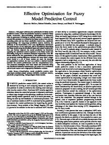
Fig. 1.
Example of a traffic network consisting of M = 6 sub-systems (intersections).
where: •
xm (k) is the state of sub-system m at time k, whereas um (k) is its control input;
•
Qm is a positive semi-definite matrix and Rm is a positive definite matrix;
•
Cm is a matrix and cm is a vector of appropriate dimensions with inequality constraints;
•
Dm is a matrix and dm is a vector of appropriate dimensions with equality constraints;
•
M = {1, . . . , M} is a set with the indices of the sub-systems; and
•
T = {0, . . . , T − 1} is the time horizon.
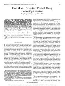
As an illustrative example, consider the traffic network depicted in Fig. 1 consisting of 13 one-way roads and 6 intersections. Sub-system 3 has state x3 = (x6 , x7 ) with estimates for the number of vehicles (queues) in roads 6 and 7, while the control vector is u3 = (u6 , u7) with the green time for each queue. The coupling graph G appears in Fig. 2. The set of input neighbors to sub-system 3 is I(3) = {1, 3, 4}. Matrix B33 expresses the discharge of queue x3 as a function of green times u3 , while B31 (B34 ) expresses how queue x3 builds up as queue x1 (x4 ) is emptied. The inequality constraints model minimum green times for each queue. The equality constraint states that the total green time plus lost time (yellow time) must add up to cycle time. This is a rough explanation of the store-and-forward model proposed in [7], [3]. March 3, 2008
DRAFT
5
x12 , x13
x10 , x11
6
x8 , x9
5
4
3 x6 , x7
1
2
x1 , x2 , x3
Fig. 2.
x4 , x5
Coupling graph for the 6-intersection traffic network.
The design of a distributed algorithm to solve P is greatly simplified by eliminating state variables through equation (2b) and collecting the variables over the horizon. Notice that subsystem m’s state at time k is a function of initial state and control signals prior to time k: xm (k) =
Akm xm (0)
+
k X X
Al−1 m Bmi ui (k − l)
l=1 i∈I(m)
¯ m and u ¯ m collect the variables over the horizon: For a compact representation, let x x (1) um (0) m .. .. ¯m = ¯m = x and u . . xm (T ) um (T − 1) And define the following matrices: Bmi 0 0 Am A B A2 Bmi 0 m mi m . .. . . ¯ .. .. . A¯m = . . and Bmi = AT −2 Bmi AT −3 Bmi AT −4 Bmi AT −1 m m m m T −2 T −1 T Am Bmi Am Bmi ATm−3 Bmi Am
...
0
0 0 ... 0 . . . Bmi
... .. .
Then it can be verified that: ¯ m = A¯m xm (0) + x
X
¯mi u ¯i B
(3)
i∈I(m)
March 3, 2008
DRAFT
6
By introducing the matrices: Qm 0 . . . 0 0 Q 0 m ... ¯m = Q . . . .. .. .. 0 0 0 0 Qm
and
¯m = R
0
Rm 0 .. .
...
Rm . . . .. . . . .
0
0
0
0
0 0 Rm
the objective term Φm is expressed as: 1 ′ ¯ 1 ′ ¯ ¯ m Qm x ¯ Rm u ¯m + u ¯m Φm = x 2 2 m X X 1 ′ ¯ 1 ¯mi u ¯ m [A¯m xm (0) + ¯mi u ¯ i ]′ Q ¯ Rm u ¯i] + u ¯m B B = [A¯m xm (0) + 2 2 m i∈I(m)
i∈I(m)
1 ¯ m A¯m xm (0) + = xm (0)′ A¯′m Q 2 1 X + 2
X
X
¯mB ¯mi u ¯i xm (0)′ A¯′m Q
i∈I(m)
i∈I(m) j∈I(m)
¯′ Q ¯ ¯ ¯j + 1 u ¯mu ¯ ′i B ¯′ R ¯m u mi m Bmj u 2 m
(4)
¯ m by replacing Φm with equation (4) and x ¯ m with equation Problem P is expressed in terms of u (3). The first term of (4) is a constant and can be disconsidered for optimization purposes. Let: ¯′ Q ¯ ¯ gmi = B mi m Am xm (0) for i ∈ I(m)
(5a)
¯′ Q ¯ ¯ Hmij = B mi m Bmj for i, j ∈ I(m), i 6= m or j 6= m
(5b)
¯′ Q ¯ ¯ ¯ Hmmm = B mm m Bmm + Rm
(5c)
Then P becomes equivalent to the following problem: X X 1 X X X ′ ′ ¯ i Hmij u ¯j + ¯i Pˆ : Min f (¯ u) = u gmi u 2 m∈M m∈M i∈I(m) j∈I(m)
(6a)
i∈I(m)
¯ m ≥ c¯m , m ∈ M S. to: C¯m u
(6b)
¯ m, m ∈ M ¯ mu ¯m = d D
(6c)
¯ = (¯ ¯ M ) is a vector with the control variables of all sub-systems over the time where u u1 , . . . , u horizon and: Cm 0 . . . 0 0 C ... 0 m C¯m = . . .. .. . . . 0 0 0 0 Cm March 3, 2008
Dm
0 ¯ , Dm = . .. 0
0
...
Dm . . . .. .. . . 0
0
0
cm
dm
c d 0 m ¯ m , c¯m = . , dm = . .. .. 0 Dm cm dm DRAFT
7
This paper is focused on the distributed solution of Pˆ with a network of distributed agents. The following sections discuss a perfect decomposition of Pˆ into a network of coupled sub-problems {Pˆm } and give a distributed iterative algorithm to solve this sub-problem network. III. P ROBLEM D ECOMPOSITION For a perfect problem decomposition, the local optimization problem of agent m must en¯ m . Before doing so, let: compass all the terms of f and constraints that depend on u •
¯ I(m) = {i : m ∈ I(i), i 6= m} be the set of output neighbors of sub-system m;
•
C(m) = {(i, j) ∈ I(m) × I(m) : i = m or j = m} be the sub-system pairs of quadratic ¯ m; terms in Φm that depend on u
•
C(m, k) = {(i, j) ∈ I(k) × I(k) : i = m or j = m} be the pairs of quadratic terms in Φk , ¯ ¯ m. k ∈ I(m), that depend on u
¯ In the traffic network, I(1) = {1}, I(1) = {2, 3, 5, 6}, C(1) = {(1, 1)}, and C(1, 3) = ¯ ¯ m appears in sub-systems i ∈ I(m) ∪ I(m), {(1, 3), (1, 4), (1, 1), (3, 1), (4, 1)}. Notice that u but can be coupled to other sub-systems—sub-system 1 is coupled to sub-system 4 via sub¯ system 3, but 4 6∈ I(1) ∪ I(1). The notion of neighborhood will establish the interdependence among sub-systems. The control variables are divided in sets according to the view of agent m: •
¯ m; local variables: the variables in vector u
•
¯ m = (¯ neighborhood variables: the variables in vector y ui : i ∈ N(m)) where N(m) = ¯ I(m) ∪ {i : (i, j) ∈ C(m, k), k ∈ I(m)} − {m} is the neighborhood of agent m. Notice ¯ that I(m) ⊆ N(m).
•
remote variables: the other variables which consist of vector z¯m = (¯ ui : i 6∈ N(m) ∪ {m}).
For a perfect problem decomposition, agent m’s problem is: 1 X ′ ¯m) = ¯ ′i Hmij u ¯ j + gmm ¯m Pˆm (¯ ym ) : Min fm (¯ um , y u u 2
(7a)
(i,j)∈C(m)
+
1 X 2 ¯
X
k∈I(m) (i,j)∈C(m,k)
March 3, 2008
¯ ′i Hkij u ¯j + u
X
′ ¯m gim u
¯ i∈I(m)
¯ m ≥ ¯cm S. to: C¯m u
(7b)
¯m ¯ mu ¯m = d D
(7c)
DRAFT
8
Problem Pˆm (¯ ym ) is further simplified using the expressions: X 1 ′ gm = (Hmim + Hmmi )¯ ui + gmm 2
(8a)
(i,m)∈C(m):i6=m
+
1 X 2 ¯
X
′ (Hkim + Hkmi )¯ ui +
k∈I(m) (i,m)∈C(m,k):i6=m
Hm = Hmmm +
X
X
gkm
¯ k∈I(m)
Hkmm
(8b)
¯ k∈I(m)
Substituting (8a) and (8b) in Pˆm (¯ ym ) leads to the reformulation: 1 ′ ′ ¯ Hm u ¯ m + gm ¯m ¯ m) = u u fm (¯ um , y 2 m ¯ m ≥ c¯m S. to: C¯m u
Pˆm (¯ ym ) : Min
¯m ¯ mu ¯m = d D
(9a) (9b) (9c)
In essence, problem Pˆm (¯ ym ) is obtained from Pˆ by i) discarding from the objective f the ¯ m and ii) dropping the constraints not associated with agent m. terms that do not depend on u Perfect decomposition means that for any agent m: ¯ m ) + f¯m (¯ f (¯ u) = fm (¯ um , y ym , ¯zm ) for an appropriate function f¯m . Hereafter {Pˆm (¯ ym )} denotes the set of problems for all m ∈ M. In what follows, we present some results relating Pˆ and the network of sub-problems. ¯ satisfies Karush-Kuhn-Tucker (KKT) first-order optimality conProposition 1: A solution u ¯ m ) satisfies KKT conditions for Pˆm (¯ ditions for Pˆ if, and only if, (¯ um , y ym ) for each m ∈ M. ¯ satisfies KKT conditions for Pˆ , then there exist Lagrangian multiplier Proof: Suppose u ≥ vectors λ= m and λm for each m ∈ M such that the following equations hold: ′ ¯m ¯′ ≥ u) = D λ= ∇u¯ m f (¯ m − C m λm
March 3, 2008
(10a)
¯ m − ¯cm ≥ 0 C¯m u
(10b)
¯m = 0 ¯ mu ¯m − d D
(10c)
λ≥ m ≥ 0
(10d)
¯ m − ¯cm )′ λ≥ (C¯m u m = 0
(10e)
DRAFT
9
¯ m ) and therefore: ¯ m ) + f¯m (¯ um , y um , y ym , ¯zm )) = ∇u¯ m fm (¯ u) = ∇u¯ m (fm (¯ Notice that ∇u¯ m f (¯ ′ ¯m ¯′ ≥ ¯ m) = D um , y λ= ∇u¯ m fm (¯ m − C m λm
(11)
Equation (11) along with equations (10b) through (10e) are precisely the KKT conditions for Pˆm (¯ ym ). The other direction can be argued in the same manner. Definition 1: (Feasible Spaces) The following sets define feasible spaces:
•
¯ m } is the feasible space for Pˆm (¯ ¯ mu ¯ m ≥ ¯cm , D ¯m = d Um = {¯ um : C¯m u ym ); U = U1 × · · · × UM is the feasible space for Pˆ ; and
•
Ym = ×i∈N (m) Ui is the feasible space for the neighborhood variables of agent m.
•
Assumption 1: (Compactness) The feasible space U is a compact set. ¯m ¯ mu ¯ ∈ U such that C¯m u ¯ m > ¯cm and D ¯m = d Assumption 2: (Strict Feasibility) There exists u for all m ∈ M. Compactness is a plausible assumption as control signals are bounded. Further, if the interior of U is empty, then some inequalities are equality constraints and should be regarded as such. Proposition 2: Pˆ is a convex problem. Proof: Problem Pˆ has a convex feasible space given by the polyhedron induced by constraints (6b) and (6c). Let the objective function of P be fP and notice that it is expressed ¯x + 1 u ¯ u for appropriate matrices Q ¯ and R, ¯ where x ¯ ′ Q¯ ¯ ′ R¯ ¯ = (¯ ¯ M ) and as fP = 12 x x1 , . . . , x 2 ¯ = (¯ ¯ M ). Equations (3) are collectively represented by x ¯ = Z¯ u ¯ +¯z for a suitable matrix u u1 , . . . , u ¯ Z¯ u ¯u = 1 u ¯ Z¯ + R)¯ ¯ u+g ¯ + ¯z)′ Q( ¯ + z¯) + 21 u ¯ ′ R¯ ¯ ′ (Z¯ ′ Q ¯ ′u ¯ +c Z¯ and a vector z¯. Clearly, fP = 12 (Z¯ u 2 ¯ is positive semi-definite and R ¯ is positive ¯ and c. fP is strictly convex because Q for some g definite. Thus, Pˆ is convex because its objective f equals fP + c. Corollary 1: Pˆm (¯ ym ) is a convex problem. Proposition 3: (Optimality Conditions) [15] Because f is a convex function and U is a convex ¯ ⋆ is a local minimum for f over U if and only if: set, u ¯ ⋆ ) ≥ 0, ∀¯ ∇f (¯ u⋆ )′ (¯ u−u u∈U
(12)
¯ ⋆ satisfying condition (12) is called a stationary point. A point u ¯ ∗ is a local minimum for Pˆ if, and only if, Corollary 2: (Local Optimality Conditions) u ¯ ∗ ) is a local minimum for Pˆm (¯ (¯ u∗ , y y⋆ ) for all m ∈ M. m
m
m
∗ ¯ is a local minimum for Pˆ such that (¯ ¯m Proof: Suppose u u∗m , y ) is not a local minimum ∗ ′ ⋆ ¯m ¯ ∗m ) < 0 for some u ˆ m ∈ Um . Note that u ˆ = u∗m , y ) (ˆ um − u for Pˆm (¯ ym ). Then ∇u¯ m fm (¯ ∗
March 3, 2008
DRAFT
10
P ¯ ∗m−1 , u ˆ m, u ¯ ∗m+1 , . . . , u ¯ ∗M ) ∈ U. And ∇f (¯ ¯ ∗) = ¯ ∗i ) = (¯ u∗1 , . . . , u u∗ )′ (ˆ u−u ∇u¯ i f (¯ u∗ )′ (ˆ ui − u i∈M P ∗ ′ ¯m ¯ ∗m ) < 0. Thus u ¯ ∗ is not a local minimum ¯ i∗ )′ (ˆ ¯ ∗i ) = ∇u¯ m fm (¯ ∇u¯ i fi (¯ u∗m , y ) (ˆ um − u u∗i , y ui − u
i∈M
for Pˆ , contradicting the hypothesis. The proof of the other direction is immediate. IV. D ISTRIBUTED O PTIMIZATION A LGORITHM
A perfect problem decomposition allows us to solve the set of problems {Pˆm } with a network of distributed agents, rather than problem Pˆ with a single, centralized agent. Herein we develop a distributed algorithm for a network of M agents to arrive at a stationary solution for {Pˆm }, (k)
(k)
¯ (k) = (¯ ¯M ) with an agent for each sub-system m. The algorithm is iterative with u u1 , . . . , u ¯ (0) , the denoting the the distributed agents’ solutions at iteration k. Starting with a feasible u agents exchange information locally about their decisions, synchronize their computations so that coupled agents do not work in parallel, and iterate until convergence is attained. Assumption 3: (Synchronous Work) If an agent m revises its decisions at iteration k then: (k)
(k)
¯ m = (¯ (i) agent m uses y ui (k+1)
¯m which becomes u
(k) : i ∈ N(m)) to obtain an approximate solution to Pˆm (¯ ym )
;
(ii) all the agents in the neighborhood of agent m keep their decisions at iteration k, that is, (k+1)
¯i u
(k)
¯i =u
for all i ∈ N(m).
¯ (k) is not a stationary point for all problems in {Pˆm }, Assumption 4: (Continuous Work) If u (k)
(k+1)
¯ m to u ¯m then at least one agent m changes its decisions from u (k) (k) ¯ m is not a stationary point to Pˆm . Pˆm (¯ ym ) such that u
by approximately solving
Condition (ii) of Assumption 3 and Assumption 4 are ensured by defining an appropriate sequence hS1 , . . . , Sr i for the agents to iterate, where Si ⊆ M, ∪ri=1 Si = M, and all distinct pairs m, n ∈ Si are non-neighbors for all i. In the illustrative example, an appropriate sequence is hS1 , S2 , S3 i where S1 = {2, 4, 6}, S2 = {1}, and S3 = {3, 5}. Other possibilities include varying sequences and the design of a protocol to meet these conditions. The details regarding synchronization and information exchange are not an issue in this paper. The rest of this section is focused on how to solve Pˆm approximately, as stated in condition (i) of Assumption 3, so ¯ (k) converges to a stationary point for {Pˆm }. that u
March 3, 2008
DRAFT
11
A. The Method of Feasible Directions ¯ (k) = u ¯ (k) , the method computes a feasible descent direction d ˆ (k) − u ¯ (k) At the current iterate u ˆ (k) subject to the original by solving a linear program that minimizes the objective ∇f (¯ u(k) )′ u ¯ (k) by finding a step α(k) that ¯ (k+1) = u ¯ (k) + α(k) d constraints. It then finds the next iterate u satisfies the Armijo Rule. The distributed method of feasible directions is detailed below. ¯ (k) 6= 0 is a feasible direction ¯ (k) ∈ U, d Definition 2: (Feasible and Descent Direction) Given u ¯ (k) ∈ U for all α > 0 that are sufficiently small. A feasible direction d ¯ (k) at ¯ (k) if u ¯ (k) + αd at u ¯ (k) < 0. ¯ (k) is a descent direction if ∇f (¯ a nonstationary point u u(k) )′ d ¯ m 6= 0 ¯ m ) ∈ Um ×Ym , d Definition 3: (Locally Feasible and Descent Direction) Given (¯ um , y (k) (k) (k) ¯ (k) ¯ m ) if u ¯ m + αm d is a locally feasible direction at (¯ um , y m ∈ Um for all αm > 0 that are (k) (k) ¯ (k) ¯ m ) is a sufficiently small. A locally feasible direction d um , y m at a nonstationary point (¯ (k)
(k)
(k)
¯ m < 0. ¯ m )′ d locally descent direction if ∇fm (¯ um , y (k)
(k)
(k)
(k) (k) (k) ¯ (k) ¯ (k) = (¯ ¯ m , ¯zm ) ∈ U, a locally descent direction d Proposition 4: Given u um , y m at the pair (k) (k) ¯ (k) = (d ¯ (k) ¯ m ) induces a descent direction d ¯ (k) . (¯ um , y m , 0, 0) at u (k) ¯ (k) ¯ (k) ¯ m + αm d Since d m is locally feasible, u m ∈ Um for all αm > 0 that are ¯ (k) ¯ (k) + α(d sufficiently small ⇒ u m , 0, 0) ∈ Um × Ym × Zm for all α > 0 sufficiently small (k) (k) (k) ¯ (k) ¯ (k) is a feasible direction at u ¯m ¯ (k) . As d ¯ m )′ d ⇒ d is locally descent, ∇fm (¯ um , y m < 0
Proof:
(k) (k) (k) (k) (k) ¯m ¯ m ), ∇y¯ m f (¯ ym , ¯zm ))′ (d , 0, 0) < 0 which implies that u(k) ), ∇¯zm f¯m (¯ um , y implies (∇u¯ m fm (¯ ¯ (k) < 0, meaning that d ¯ (k) is a descent direction at u ¯ (k) . ∇f (¯ uk )′ d
There is an equivalent way to define feasible and descent directions for convex problems that simplifies algorithm design. Details are given for global directions but the concepts are easily ¯ (k) at u ¯ (k) are vectors of the form: extendible to local directions. The feasible directions d ¯ (k) = γ(ˆ ¯ (k) ), γ > 0 d u(k) − u ˆ (k) ∈ U is a feasible point not equal to u ¯ (k) . The method produces iterates as follows: where u ¯ (k+1) = u ¯ (k) + α(k) (ˆ ¯ (k) ) u u(k) − u
(13)
ˆ (k) ∈ U, and if u ¯ (k) is nonstationary: where α(k) ∈ (0, 1], u ¯ (k) ) < 0 ∇f (¯ u(k) )′ (ˆ u(k) − u
March 3, 2008
DRAFT
12
¯ (k) + α(k) (ˆ ¯ (k) ) ∈ U for all α(k) ∈ [0, 1] since U is convex and u ˆ (k) , The next iterate u u(k) − u ¯ (k) ∈ U. Thus, all iterates of the sequence {¯ ¯ (k) is not stationary, there u u(k) } are feasible. If u ˆ (k) ∈ U that induces a descent direction or else ∇f (¯ ¯ (k) ) ≥ 0, ∀¯ exists u u(k) )′ (¯ u−u u ∈ U. Besides the computation of descent directions, which is often problem dependent and will be discussed later, stepsize selection is critical to ensure convergence to a stationary point. Among the existing rules for stepsize selection, we adopt the Armijo Rule for its simplicity. This rules fixes scalar parameters β, σ ∈ (0, 1) and chooses the stepsize α(k) = β sk where sk is the smallest nonnegative integer s for which: ¯ (k) )) ≤ f (¯ ¯ (k) ) f (¯ u(k) + β s (ˆ u(k) − u u(k) ) + σβ s ∇f (¯ u(k) )′ (ˆ u(k) − u
(14)
A key issue is whether each limit point of a sequence {¯ u(k) } generated by the feasible direction method is a stationary point. From first-order Taylor’s expansion f (¯ u(k+1) ) = f (¯ u(k) )+ ¯ (k) . If the slope of f at u ¯ (k) , which is given by ∇f (¯ ¯ (k) , ¯ (k) along direction d α(k) ∇f (¯ u(k) )′ d u(k) )′ d has substantial magnitude, the rate of convergence of the method tends to be substantial as well. ¯ (k) become asymptotically orthogonal to the gradient direction as However, if the directions d ¯ (k) will tend to zero and the ¯ (k) is drawn to a nonstationary point, then the slope ∇f (¯ u u(k) )′ d ¯ (k) method may get stuck near that point. Conditions are therefore imposed on the directions d ¯ (k) is a function of the to preclude such undesirable behavior. These conditions assume that d ¯ (k) and, typically, are satisfied or easily enforced by the algorithms. One corresponding iterate u such condition is the concept of gradient related sequence [15] stated below. ¯ (k) } be the sequence of directions and let Definition 4: (Gradient Related Sequence) Let {d {¯ u(k) } be the associated sequence of solutions generated by the feasible direction method (13). ¯ (k) } is gradient related to {¯ The sequence {d u(k) } if for any subsequence {¯ u(k) }k∈K that converges ¯ (k) }k∈K is bounded and satisfies: to a nonstationary point, the corresponding subsequence {d ¯ (k) < 0 lim sup ∇f (¯ u(k) )′ d
k→∞ k∈K ¯ (k)
For a gradient related sequence {d }, if the subsequence {∇f (¯ u(k) )}k∈K tends to a nonzero ¯ (k) }k∈K is bounded and does not tend to be orthogonal to ∇f (¯ vector, then {d u(k) ). A gradient related sequence is obtained by imposing certain conditions on direction computation. Let us start with the proposition below which comes from the theory presented in [15, Sec. 2.2.1]. Proposition 5: (Stationarity of Limit Points) Let {¯ u(k) } be a sequence yielded by the feasible ¯ (k) } is gradient related to {¯ direction method (13). Suppose {d u(k) } and α(k) is chosen by the March 3, 2008
DRAFT
13
Armijo rule. Then every limit point of {¯ u(k) } is a stationary point for Pˆ . Corollary 3: (Stationarity of Limit Points for the Distributed Method) Suppose that: 1) {¯ u(k) } is a sequence generated by the distributed agents under Assumptions 3 and 4; (k+1) (k) ¯ m to Pˆm (¯ 2) agent m gets an approximate solution u ym ) with the feasible direction method: (k) (k) (k) (k) ¯ (k+1) ¯m ¯m u =u + αm (ˆ um −u ) m
(15a)
(k) (k) (k) (k) ¯m ˆm − u ¯ m , for u ˆ m ∈ Um , and the stepsize where the local descent direction is d =u (k)
(k)
smk αm ∈ (0, 1] satisfies the Armijo rule, that is, αm = βm for some βm , σm ∈ (0, 1) where
smk is the smallest nonnegative integer sm for which: sm ¯ (k) (k) (k) (k) sm (k) ′ ¯ (k) ¯m ¯m ¯m fm (¯ u(k) ) ≤ fm (¯ um ,y ) + σm βm ∇fm (¯ u(k) ) dm m + βm dm , y m ,y
(15b)
¯ (k) } is gradient related to {¯ 3) the sequence {d u(k) }. Then every limit point of {¯ u(k) } is a stationary point for Pˆ . Proof: The assumption of perfect problem decomposition, given by equations (9a) through (9c), and Assumption 3 ensure that the iterations of the agents are decoupled, allowing us to assume that only one agent updates its decision at iteration k, say agent m, for the purpose of convergence analysis. These assumptions together with Assumption 4 ensure that agent m yields (k) (k) ¯ (k+1) ¯m a new iterate u at a nonstationary point (¯ um , y ) for Pˆm . m (k) (k) (k) (k) ¯m ¯ m ) is also According to Proposition 4, the local descent direction d for Pˆm (¯ ym ) at (¯ um , y ¯ (k) . Because agent m satisfies the Armijo rule (15b): a descent direction for Pˆ at u (k)
(k)
(k)
(k)
(k)
(k)
(k)
(k)
smk ¯ smk ¯m ¯ m ) ≤ fm (¯ ¯ m ) + σm βm ¯ m )′ d fm (¯ um + βm dm , y um , y ∇fm (¯ um , y
⇒ (k)
(k)
(k)
(k)
(k)
(k)
(k)
(k)
(k)
smk ¯ ¯ m ) + f¯m (¯ ¯ m ) + f¯m (¯ fm (¯ um + βm dm , y ym , ¯zm ) ≤ fm (¯ um , y ym , z¯m ) (k) (k) (k) ¯ (k) ¯ m ), ∇y¯ m f (¯ ym , z¯k ))′ (d u(k) ), ∇¯zm f¯m (¯ um , y +σm β smk (∇u¯ m fm (¯ m , 0, 0) m
m
⇒ smk ¯ (k) smk ¯ (k) f (¯ u(k) + βm d ) ≤ f (¯ u(k) ) + σm βm ∇f (¯ u(k) )′ d
¯ (k) = (d ¯ (k) where d m , 0, 0), implying that the Armijo rule (14) is also satisfied. From assumption (k) ¯ (k) } = {(d ¯m 3 of this corollary, sequence {d , 0, 0)} of descent directions is gradient related (k)
(k)
k ¯m to sequence {¯ u(k) } = {(¯ um , y , ¯zm )} of solutions yielded by the distributed agents. Hence, Proposition 5 ensures that every limit point of {¯ u(k) } is a stationary point for Pˆ .
Condition 3 of Corollary 3 is ensured by appropriate computation of the feasible descent direction, which is the topic of the remainder of this section. March 3, 2008
DRAFT
14
B. Descent Direction Computation (k) (k) (k) (k) ¯m ¯ m ) that is gradient related The computation of a descent direction d for Pˆm (¯ ym ) at (¯ um , y (k) (k) ¯ (k) ˆ m ˆ (k) ¯m is discussed here. Actually, a point u −u is computed by solving: m such that dm = u (k) ˆ m (¯ ¯m D u(k) ) : Min m ,y
(k) ′ (k) ¯m ¯ (k) u(k) ) (ˆ um −u ∇u¯ m fm (¯ m ,y m )
(16a)
ˆ (k) S. to: C¯m u cm m ≥ ¯
(16b)
¯ ¯ mu ˆ (k) D m = dm
(16c)
(k) ˆ m is a linear program solvable with ˆ m as decision variables. Notice that D which has vector u ˆ m has a nonnegative standard linear programming (LP) algorithms. If the optimal solution to D (k) (k) (k) (k) (k) (k) ¯ m )′ (ˆ ¯ m ) ≥ 0 for all ¯ m ) is locally optimal for Pˆm : ∇u¯ m fm (¯ um , y um − u objective, then (¯ um , y (k) (k) (k) ¯ (k) ˆ m ∈ Um . Otherwise, d ˆm − u ¯ m is a descent direction. u m = u
¯ (k) } = {(d ¯ (k) It remains to show that the direction sequence {d m , 0, 0)} obtained by solving ˆ m is gradient related to {¯ ˜ for D u(k) }. Suppose that {¯ u(k) } converges to a nonstationary point u a subsequence K. Then, we must show that: ¯ (k) k = lim sup kˆ ¯ (k) k < ∞ lim sup kd u(k) − u
k→∞ k∈K
k→∞ k∈K
¯ (k) = lim sup ∇f (¯ ¯ (k) ) < 0 lim sup ∇f (¯ u(k) )′ d u(k) )′ (ˆ u(k) − u
k→∞ k∈K
k→∞ k∈K
(17a) (17b)
Assume w.l.o.g. that only an agent updates its decisions, say agent m(k), at iteration k. Note (k)
(k)
(k)
(k)
¯ (k) k = kˆ ¯ m(k) k. Condition (17a) holds since u ˆ m(k) , u ¯ m(k) ∈ Um(k) and that kˆ u(k) − u um(k) − u (k) ˆ m: ˆ Um(k) is compact (Assumption 1). It follows from the optimality of u with respect to D m(k)
(k)
(k)
¯ (k) ) = ∇fm(k) (¯ ¯ m(k) ) ∇f (¯ u(k) )′ (ˆ u(k) − u u(k) )′ (ˆ um(k) − u (k)
¯ m(k) ), ∀¯ ≤ ∇fm(k) (¯ u(k) )′ (¯ um(k) − u um(k) ∈ Um(k) By applying the limit we obtain: ˜ m ) for some m < 0 ¯ (k) ) ≤ min ∇fm (˜ u)′ (¯ um − u lim sup ∇f (¯ u(k) )′ (ˆ u(k) − u
k→∞ k∈K
¯ m ∈Um u
which proves condition (17b). We now consider a particular type of problem Pˆ in which Cm is the identity matrix, cm = 0, Dm = 1′ is a row vector, and dm = dm is a scalar for all m ∈ M. This particular problem is
March 3, 2008
DRAFT
15
of interest in the application to urban traffic control, where constraints (2c) and (2d) can be: um (k) ≥ 0, ∀m ∈ M, k ∈ T
(18a)
1′ um (k) = dm , ∀m ∈ M, k ∈ T
(18b)
In such situation, variables um (k) represent the extra time given to a phase beyond the minimum. (k) ¯ (k) ˆ ym This constraint structure simplifies the computation of a descent direction d ) at m for Pm (¯ (k)
(k)
¯ m ). Let u ¯ m = (¯ ¯ m (T − 1)) and u ¯ m (t) = (um1 (t), . . . , uml(m) (t)) where l(m) (¯ um , y um (0), . . . , u ˆ m has exactly one nonzero variable ¯ m (t). A basis for the LP problem D is the dimension of u (k) (k) ym ) is obtained analytically as: uˆmi (t) for each t ∈ T . Hence, the optimal solution to Pˆm (¯
∂ (k) ¯m i⋆ (t) = arg min fm (¯ u(k) ) m ,y 1≤i≤l(m) ∂umi (t) 0, i 6= i⋆ (t) (k) dmi (t) = dm , i = i⋆ (t)
(19a)
(19b)
(k) (k) (k) ¯m ¯ (k) ¯ (k) ¯ (k) where d (t) = (dm1 (t), . . . , dml(m) (t)) and d m = (dm (0), . . . , dm (T − 1)).
V. N UMERICAL I LLUSTRATION This section reports results from the application of distributed MPC to the urban traffic network depicted in Fig. 2. The state variable x(k) represents the queues of vehicles in each road. As traffic lights are the actuators, the control problem consists in the green time, u(k), designated to each stream of vehicles. This control problem may be expressed in terms of objective (2a), subject to constraints (2b) through (2d) as control signals must lie within bounds and hold constant cycle periods. Although such problem is typically solved by an LQR regulator where constraints are imposed in an ad-hoc manner [7], recent works indicate that substantial gains are achieved with sliding-horizon control methods such as MPC [16], [17]. However, the standard MPC framework solves QP problems whose complexity increases with the number of variables and prediction horizon. Further, large networks require extensive exchange of messages, centralized around the peer responsible for the solution of the global problem. In this context, distributed MPC may circumvent the complexity of operating large networks by solving smaller, interconnected optimization problems and exchanging information among neighboring agents. The distributed MPC framework with a prediction horizon of 5 steps was applied to solve a single time step of the traffic network (Fig. 2) with two distributed optimization algorithms: March 3, 2008
DRAFT
16
TABLE I C OMPUTATIONAL RESULTS FOR A SET OF 10
INITIAL CONDITIONS WITH
Quadratic Programming CPU Time (ms)
1% ERROR TOLERANCE .
Feasible Direction
Iterations
CPU Time (s)
Iterations
Mean
Max
Mean
Max
Mean
Max
Mean
Max
Agent 1
21.9
93.8
1.6
3
0.35
0.78
13.4
30
Agent 2
9.4
31.2
1.1
2
0.24
0.45
10.2
20
Agent 3
1.6
15.6
1.7
4
0.24
0.53
9.5
20
Agent 4
7.8
46.9
1.6
3
0.22
0.28
14.4
24
Agent 5
3.1
15.6
1.5
3
0.26
0.55
10.0
20
Agent 6
3.1
15.6
0.8
2
0.20
0.48
8.3
20
Distributed
46.9
125.0
8.3
14
1.55
3.08
63.7
130
Centralized
26.6
46.9
3.9
7
0.40
1.94
12.0
58
TABLE II C OMPUTATIONAL RESULTS FOR A SET OF 10
INITIAL CONDITIONS WITH
Quadratic Programming CPU Time (ms)
0.1% ERROR TOLERANCE .
Feasible Direction
Iterations
CPU Time (s)
Iterations
Mean
Max
Mean
Max
Mean
Max
Mean
Max
Agent 1
21.9
46.9
3.3
7
2.16
8.12
76
290
Agent 2
15.6
46.9
2.1
4
1.98
8.20
72
290
Agent 3
10.9
46.9
2.8
8
1.85
7.59
69
280
Agent 4
14.1
31.2
3.0
6
1.85
7.50
76
294
Agent 5
1.6
15.6
2.4
5
1.83
7.70
69
280
Agent 6
6.3
46.9
1.2
2
1.81
7.67
67
280
Distributed
75.0
156.2
14.8
25
11.58
47.16
425
1710
Centralized
26.6
46.9
3.9
7
13.59
48.09
370.9
1299
the distributed feasible direction method given in Sec. IV and the distributed solution with a standard QP algorithm1. In both cases the centralized solution was also computed for comparison purposes. As convergence rate depends on the method and initial conditions, the results are shown for a set of 10 initial queues obtained at random. 1
For the distributed feasible direction method, experiments showed that the parameters σ = 0.3 and β = 0.3 induce the best
convergence rate in the given scenario. Notice that the distributed QP approach also implicitly satisfies local Armijo rules.
March 3, 2008
DRAFT
17
14
·10 7 Centralized QP Distributed QP (0.1% error) Distributed QP (1% error) LQR
12
Cost
10 8 6 4 2 0
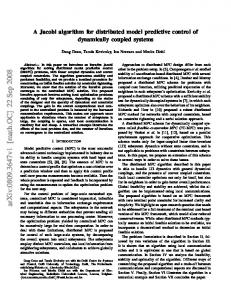
Fig. 3.
1
2
3
Prediction Horizon
4
5
Mean accumulated cost of objective function for 10 initial conditions and 5 prediction horizons.
Specially for practical purposes, it is important to present the number of iterations a method takes before reaching a solution within a desired tolerance from the optimal. Thus, optimizations were performed for two different error margins. Results presented in Table I assume that objective costs are within 1% of the optimal, whereas in Table II they are at most 0.1% from the optimal. In both cases the centralized QP approach arrived at an optimal solution, as the algorithm was allowed to iterate until satisfying optimality conditions. As previously remarked, the MPC framework can improve the operation of traffic networks, but it is yet to be confirmed in traffic simulators or real urban sites. Fig. 3 gives the mean accumulated cost of the network’s objective function, using the same set of initial conditions as before, over a 40-step simulation time frame and for different prediction horizons. The MPC reduction on the accumulated cost is very considerable when compared to the LQR approach, of approximately 10% with a proper prediction horizon for this example. Although such results derive from a model-based simulation, the cost reduction praises the usefulness of the distribued MPC approach instigating further analysis with specialized simulation tools.
March 3, 2008
DRAFT
18
VI. S UMMARY The MPC framework applied to the quadratic regulation problem of linear dynamic networks solves a series of QP problems. The network structure of these QP problems allows its decomposition into a network of locally coupled sub-problems. This paper developed a distributed version of the method of feasible directions for the network of sub-problems that ensures converge to a solution. The distributed algorithm solves relatively simple local problems at the expense of high local communications and slower convergence rate. Some numerical results are reported from the application of the distributed MPC approach to the TUC split control of urban traffic networks. Future work will apply distributed MPC to urban traffic control in simulated scenarios and introduce local constraints on state variables. R EFERENCES [1] S. J. Qin and T. A. Badgwel, “A survey of industrial model predictive control technology,” Control Engineering Practice, vol. 11, no. 7, pp. 733–764, 2003. [2] E. F. Camacho and C. Bordons, Model Predictive Control. Springer-Verlag, 2004. [3] M. Papageorgiou, C. Diakaki, V. Dinopoulou, A. Kotsialos, and Y. Wang, “Review of road traffic control strategies,” IEEE Proceedings, vol. 91, no. 12, pp. 2043–2067, 2003. [4] J. Nocedal and S. J. Wright, Numerical Optimization. Springer-Verlag, 1999. [5] E. Camponogara, D. Jia, B. H. Krogh, and S. N. Talukdar, “Distributed model predictive control,” IEEE Control Systems Magazine, vol. 22, no. 1, pp. 44–52, February 2002. [6] E. Camponogara and S. N. Talukdar, “Distributed model predictive control: synchronous and asynchronous computation,” IEEE Transactions on Systems, Man, and Cybernetics – Part A, vol. 37, no. 5, pp. 732–745, September 2007. [7] C. Diakaki, M. Papageorgiou, and K. Aboudolas, “A multivariable regulator approach to traffic-responsive network-wide signal control,” Control Engineering Practice, vol. 10, no. 2, pp. 183–195, 2002. [8] M. Mercang¨oz and F. J. Doyle, “Distributed model predictive control of an experimental four-tank system,” Journal of Process Control, vol. 17, no. 3, pp. 297–308, 2007. [9] S. Talukdar, D. Jia, P. Hines, and B. H. Krogh, “Distributed model predictive control for the mitigation of cascading failures,” in Proc. of the 44th IEEE Conference on Decision and Control, and the European Control Conference, 2005, pp. 4440–4445. [10] W. B. Dunbar and R. M. Murray, “Distributed receding horizon control for multi-vehicle formation stabilization,” Automatica, vol. 42, pp. 549–558, 2006. [11] T. Keviczky, F. Borrelli, and G. J. Balas, “Decentralized receding horizon control for large scale dynamically decoupled systems,” Automatica, vol. 42, pp. 2105–2115, 2006. [12] S. Li, Y. Zhang, and Q. Zhu, “Nash-optimization enhanced distributed model predictive control applied to the shell benchmark problem,” Information Sciences, vol. 170, pp. 259–349, 2005. [13] A. N. Venkat, J. B. Rawlings, and S. J. Wright, “Stability and optimality of distributed model predictive control,” in Proc. of the 44th IEEE Conference on Decision and Control, and the European Control Conference, 2005, pp. 6680–6685. March 3, 2008
DRAFT
19
[14] R. R. Negenborn, B. D. Schutter, and J. Hellendoorn, “Multi-agent model predictive control for transportation networks: serial versus parallel schemes,” to appear in Engineering Applications of Artificial Intelligence, 2007. [15] D. P. Bertsekas, Nonlinear Programming.
Belmont, MA: Athena Scientific, 1995.
[16] L. B. de Oliveira and E. Camponogara, “Predictive control for urban traffic networks: initial evaluation,” in Proceedings of the 3rd IFAC Symposium on System, Structure and Control, Iguassu, Brazil, 2007. [17] K. Aboudolas, M. Papageorgiou, and E. Kosmatopoulos, “Control and optimization methods for traffic signal control in large-scale congested urban road networks,” in Proceedings of the American Control Conference, New York, USA, July 2007, pp. 3132–3138.
March 3, 2008
DRAFT