Distributed Programming over Time-series Graphs - Department of

Distributed Programming over Time-series Graphs Yogesh Simmhan, Neel Choudhury

Charith Wickramaarachchi, Alok Kumbhare, Marc Frincu, Cauligi Raghavendra, Viktor Prasanna

Indian Institute of Science, Bangalore 560012 India [email protected], [email protected]

Univ. of Southern California, Los Angeles CA 90089 USA {cwickram,kumbhare,frincu,raghu,prasanna}@usc.edu

Abstract—Graphs are a key form of Big Data, and performing scalable analytics over them is invaluable to many domains. There is an emerging class of inter-connected data which accumulates or varies over time, and on which novel algorithms both over the network structure and across the time-variant attribute values is necessary. We formalize the notion of time-series graphs and propose a Temporally Iterative BSP programming abstraction to develop algorithms on such datasets using several design patterns. Our abstractions leverage a sub-graph centric programming model and extend it to the temporal dimension. We present three time-series graph algorithms based on these design patterns and abstractions, and analyze their performance using the GoFFish distributed platform on Amazon AWS Cloud. Our results demonstrate the efficacy of the abstractions to develop practical time-series graph algorithms, and scale them on commodity hardware.

I. I NTRODUCTION There is a rapid proliferation of ubiquitous physical sensors, personal devices and virtual agents that sense, monitor and track human and environmental activity as part of the evolving Internet of Things (IoT) [1]. Data streaming continuously or periodically from such domains are intrinsically interconnected and grow immensely in size. These often possess two key characteristics: (1) temporal attributes and (2) network relationships that exist between them. Such datasets that imbue both these temporal and graph features have not been adequately examined in Big Data literature even as they are becoming pervasive. For example, consider a road network in a Smart City. The road topology remains relatively static over days. However, the traffic volume monitored on each road segment changes significantly throughout the day [2], as do the actual vehicles that are captured by traffic cameras. Widespread urban monitoring systems, community mapping apps 1 , and the advent of self-driving cars will continue to enhance our ability to rapidly capture changing road information for both realtime and offline analytics. There are many similar network datasets where the graph topology changes incrementally but attributes of vertices and edges vary often. These include Smart Power Grids (changing power flows on edges, power consumption at vertices), communication infrastructure (varying edge bandwidths between endpoints) [3], and environmental sensor networks (real-time observations from sensor vertices). Despite their seeming dynamism, even social network graph structures change more slowly compared to the number of 1 https://www.waze.com/

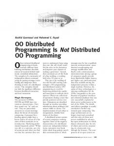
tweets or messages exchanged over the network 2 . Analytics that range from intelligent traffic routing to epidemiology studies on how diseases spread are possible on these. Graph datasets with temporal characteristics have been variously known in literature as temporal graphs [4], kineographs [5], dynamic graphs [6] and time-evolving graphs [7]. Temporal graphs capture the time variant network structure in a single graph by introducing a temporal edge between the same vertex at different moments. Others construct graph snapshots at specific change points in the graph structure, while Kineograph deal with graph that exhibit high structural dynamism. As such, the exploration into such graphs with temporal features is at an early stage (§ V). In this paper, we focus on the subset of batch processing over time-series graphs. We define time-series graphs as those whose network topology is slow-changing but whose attribute values associated with vertices and edges change (or are generated) much more frequently. As a result, we have a series of graphs accumulated over time, each of whose vertex and edge attributes capture the historic states of the network at points in time (e.g. the travel time on edges of a road network at 3PM on 2 Oct, 2014), or its cumulative states over time durations (e.g. the license plates of vehicles seen at a road crossing vertex between 3:00PM–3:05 on 2 Oct, 2014), but whose number of, and connectivity between, vertices and edges are less dynamic. Each graph in the time-series is an instance – and we may have thousands to millions of these instances over time, while the slow changing topology is a template – with millions to billions of vertices and edges. Fig. 1 shows a graph template that captures the network structure and schema of the vertex and edge attributes, while the instances show the timestamped values for these vertices and edges. There is limited work on distributed programming models and algorithms to perform analytics over such time-series graphs. The recent emphasis on distributed graph frameworks using iterative vertex-centric [8], [9] and partition-centric [10] programming models are limited to single, large graphs. Our recent work on GoFFish introduced a subgraph-centric pro2 Each of the 1.3B Facebook users (vertices) with an average of 130 friends each (edge degree) create about 3 objects per day, or 4B objects per day (http://bit.ly/1odt5aK). In comparison, about 144M edges are added each day to the existing 169B edges, for about 1% of daily edge topology change (http://bit.ly/1diZm5O), and about 14% new users were added in the 12 months, or about 0.04% vertex topology change per day (http://bit.ly/1fiOA4J)

*

)*

Graph Template

Graph Instances

Graph ID, 34567890 Time, start, duration (Attribute Name, Value)*

Graph ID, Long (Attribute Name, Type)*

)*

time Vertex ID, Long (Attribute Name, Type)*

Edge ID, Long (Attribute Name, Type)*

…

Vertex ID, 12345678 (Attribute Name, Type)*

each vertex vit ∈ V t for a graph instance g t at time t has a set of attribute values {b vi .id, vit .αk , . . . , vit .αm }, and each edge t t ej ∈ E has attribute values {b ej .id, etj .βl , . . . , etj .βn }. Note that while the template is invariant, a slow changing topology can be captured using an isExists attribute that simulates the appearance (isExists=true) or disappearance (isExists=false) of vertices or edges at different instances.

Edge ID, 23456789 (Attribute Name, Type)*

Figure 1. Time-series graph collection. Template captures static topology and attribute names. Instances record temporally variant attribute values.

gramming model [11] and algorithms [12] over single, distributed graphs that significantly out-performs vertex-centric models. In this paper, we focus on a programming model for analysis over a collection of distributed time-series graphs, and develop graph algorithms that benefit from them. In particular, we target applications where the result of computation on a graph instance in one timestep is necessary to process a graph instance in the next timestep [13]. We refer to this class of algorithm as sequentially-dependent temporal graph algorithms, or simply, sequentially-dependent algorithms. We make the following specific contributions in this paper: 1) We define a time-series graph data model, and propose a Temporally Iterative Bulk Synchronous Parallel (TIBSP) programming abstraction to support several design patterns for temporal graph algorithms (§ II); 2) We develop three time-series graph algorithms that benefit from these abstractions: Time-Dependent Shortest Path, Meme Tracking, and Hashtag Aggregation (§ III); 3) We empirically evaluate and analyze these three algorithms on GoFFish, a distributed graph processing framework that implements the TI-BSP abstraction. (§ IV). II. P ROGRAMMING OVER T IME - SERIES G RAPHS A. Time-series Graphs We define a collection of time-series graphs as Γ = b G, t0 , δi, where G b is a graph template – the time invariant hG, topology, and G is an ordered set of graph instances, capturing b = hVb , Ei b time-variant values ranging from t0 in steps of δ. G b b b gives the set of vertices, vbi ∈ V , and edges, ebj ∈ E : V → Vb , common to all graph instances. The graph instance g t ∈ G at timestamp t is given by hV t , E t , ti where vit ∈ V t and etj ∈ E t capture the vertex and b at time t, respectively. edge values for vbi ∈ Vb and ebj ∈ E b The set G is ordered in time, |V t | = |Vb | and |E t | = |E|. starting from t0 . Time-series graphs are often periodic, in that the instances are captured at regular intervals. The constant period between successive instances is δ, i.e., ti+1 − ti = δ. Vertices and edges in the template have a defined set of b = typed attributes, A(Vb ) = {id, α1 , . . . , αm } and A(E) {id, β1 , . . . , βn } respectively. All vertices of the graph template share the same set of attributes, as do edges, with id being the unique identifier. Graph instances have values for each attribute in their vertices and edges. The id attribute’s value is static across instances, and is set in the template. Thus

B. Design Patterns for Time-series Graph Algorithms Graph algorithms can be classified into traversal, centrality measures, and clustering, among others, and these are well studied. With time-series graphs, it helps to understand the design pattern of an algorithm when operating over instances. In traversal algorithms for time-series graphs, in addition to traversing along the edges of the graph topology, one can also traverse along the time dimension. One approach is to consider a “virtual” directed temporal edge from one vertex in a graph instance at time ti to the same vertex in the next instance at ti+1 . Thus, we can traverse either on one spatial or on one temporal edge at a time, and this enables algorithms such as shortest path over time and information propagation (§ III). This also introduces a temporal dependency in the algorithm since the acyclic temporal edges are directed forward in time. Likewise, one may gather statistics over different graph instances and finally aggregate them, or perform clustering on each instance and find their intersection to show how communities evolve. Here, the initial statistic or clustering can happen independently on each instance, but a merge step would perform the aggregation (§ III). Further, there are also algorithms where each graph instance is treated independently, such as when gathering independent statistics on each instance. Even a complex analytic, such as finding the daily Top-N central vertices in a year to visualize traffic flows, can be done in a pleasingly temporally parallel manner. Based on these motivating examples, we synthesize three design patterns for temporal graph algorithms (Fig. 2). 1) Analysis over every graph instance is independent. The result from the application is just a union of results from each graph instance; 2) Graph instances are eventually dependent. Each instance can execute independently but results from all instances are aggregated in a Merge step to produce the final result; 3) Graph instances are sequentially dependent over time. Here, analysis over a graph instance cannot start (or, alternatively, complete) before the results from the previous graph instance are available. While not meant to be comprehensive, identifying these patterns serves two purposes: (1) To make it easy for algorithm designers to think about time-series graphs on which there is limited literature, and (2) To make it possible to efficiently scale them in a distributed environment. Of these patterns, we particularly focus on the sequentially dependent pattern since it is intrinsically tied to the time-series nature of the graphs.

Graph Instance T0

Graph Instance T0

Graph Instance T0

Read Instance 1 BSP GoFS

Graph Instance T1

Graph Instance T3

Graph Instance Tn

Graph Instance Tn

Merge

Graph Instance T1

TIMESTEP 1

Graph Instance T1

Graph Instance T3

Graph Instance Tn

SUPERSTEP N

Read Instance 2 BSP

C. Subgraph-Centric Programming Abstraction Vertex-centric distributed graph programming models [8], [9], [14] have become popular due to their ease of defining a graph algorithm from a vertex’s perspective. These have been extended to partition-, block- and subgraph-centric abstractions [10], [11], [15] with significant performance benefits. We build upon our subgraph-centric programming model to support the proposed design pattern for time-series graphs [11]. We recap its Bulk Synchronous Parallel (BSP) model and then describe our novel Temporally Iterative BSP (TI-BSP) model. A subgraph-centric programming model defines the graph application logic from the perspective of a single subgraph within a partitioned graph. A graph G = hV, Ei is partitioned into n partitions, hP1 = (V1 , E1 ), · · · , Pn = (Vn , En )i such n n S S that Vi = V , Ei = E, and ∀i 6= j : Vi ∩ Vj = ∅, i.e. i=1

i=1

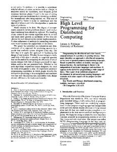
a vertex is present in only one partition, and an edge appears in only one partition, except for “remote” edges that can span two partitions. Conversely, “local” edges for a partition are those that connect vertices within the same partition. Typically, partitioning tries to ensure that the number of vertices, |Vi |, is equal Pn across partitions and the total number of remote edges, i=1 |Ri |, is minimized. A subgraph within a partition is a maximal set of vertices that are weakly connected through only local edges. A partition i has between 1 and |Vi | subgraphs. In subgraph-centric programming, the user defines an application logic as a Compute method that operates on a single subgraph, independently. The method, upon completion, can exchange messages with other subgraphs, typically those that share a remote edge. A single execution of the Compute method on all subgraphs, each of which can execute concurrently, forms a superstep. Execution proceeds as a series of barriered supersteps, executed in a BSP model. Messages generated in one superstep are transmitted in “bulk” between supersteps, and available to the Compute of the destination subgraph in the next superstep. The Compute method for a subgraph can VoteToHalt. Execution stops when all subgraphs VoteToHalt in a superstep and they have not generated any messages. Each gray box (timestep) in Fig. 3 illustrates this BSP execution model. The subgraph-centric model [11] is itself an extension of the vertex-centric model (where the Compute logic is defined for a single vertex [9]), and offers better relative performance.

Send messages across iterations

Send messages between supersteps

BSP BSP

Sequentially Dependent iBSP

Figure 2. Design patterns for time-series graph algorithms.

TIMESTEP M TIMESTEP 2

SEQUENTIALLY DEPENDENT

SUPERSTEP 1 SUPERSTEP 2

GoFS

EVENTUALLY DEPENDENT

INDEPENDENT

Sub-graphs in Partition

Figure 3. TI-BSP model. Each BSP timestep operates on a single graph instance, and is decomposed into multiple supersteps as part of the subgraphcentric model. Graph instances are initialized at the start of each timestep.

D. Temporally Iterative BSP (TI-BSP) for Time-series Graphs Subgraph-centric BSP programming offers natural parallelism across the graph topology. But it operates on a single graph, i.e., corresponding to one box in Fig. 2 that operates on a single instance. We use BSP as a building block to propose a Temporally Iterative BSP (TI-BSP) abstraction that supports the design patterns. A TI-BSP application is a set of BSP iterations, each referred to as a timestep since it operates on a single graph instance in time. While operations within a timestep could be opaque, we use the subgraph-centric abstraction consisting of BSP supersteps as the constituents of a timestep. In a way, the timesteps over instances form an outer loop, while the supersteps over subgraphs of an instance are the inner loop (Fig. 3). The execution order of the timesteps and the messaging between them decides the design pattern. Synchronization and Concurrency. A TI-BSP application operates over a graph collection, Γ, which, as defined earlier, is a list of time ordered graph instances. As before, users implement a Compute method which is invoked on every subgraph and for every graph instance. In case of an eventually dependent pattern, users provide an additional Merge() method for invocation after all instance timesteps complete. For a sequentially dependent pattern, only one graph instance and hence one BSP timestep is active at a time. The Compute method is called on all subgraphs of the first instance to initiate the BSP. After the completion of those supersteps, the Compute method is called on all subgraphs of the next instance for the next timestep iteration, and so on till the last graph instance is reached. Users may also VoteToHaltTimestep(); the timesteps are run on either a fixed number of graph instances like a For loop (e.g., a time range, ti ..ti+20 ), or until all subgraphs VoteToHaltTimestep and no new messages are emitted, similar to a While loop. Though there is spatial concurrency across subgraphs in a BSP superstep, each timestep iteration is itself sequentially executed after the previous.

In case of an independent pattern, the Compute method can be called on any graph instance independently, as long as the BSP is run on each instance exactly once. The application terminates when the timesteps on all the identified instance time range complete. Here, we can exploit both spatial concurrency across subgraphs and temporal concurrency across instances. An eventually dependent pattern is similar, except that the Merge method is called after the timesteps complete on all instances in the identified time range within the collection. The parallelism is similar to the independent pattern, except for the Merge BSP supersteps which are executed at the end. User Logic. The signatures of the Compute method and the Merge method (in case of an eventually dependent pattern) implemented by the user is given below. We also introduce an EndOfTimestep() method the user can implement; it is invoked at the end of each timestep. The parameters are passed to these methods by the execution framework. Compute(Subgraph sg, int timestep, int superstep, Message[] msgs) EndOfTimestep(Subgraph sg, int timestep) Merge(SubgraphTemplate sgt, int superstep, Message[] msgs)

Here, the Subgraph has the time variant attribute values of the corresponding graph instance for this BSP in addition to the subgraph topology that is time invariant. The timestep corresponds to the graph instance’s index relative to the initial instance ti , while the superstep corresponds to the superstep number inside the BSP execution. If the superstep number is 1, it indicates the start of an instance’s execution, i.e., timestep. Thus it offers a context for interpreting the list of messages, msgs. In case of a sequentially dependent application pattern, messages received when superstep=1 have arrived from its preceding BSP instance upon its completion. Hence, it indicates the completion of the previous timestep, the start of the next timestep and helps to pass the state from one instance to the next. If, in addition, the timestep=1, then this is the first BSP timestep and the messages are the inputs passed to the application. For an independent or eventually dependent pattern, messages received when the superstep=1 are application input messages since there is no notion of a previous instance. In cases where superstep>1, these are messages received from the previous superstep inside a BSP. Message Passing. Besides messaging between subgraphs in supersteps supported by the subgraph-centric abstraction, we introduce additional message passing and application termination constructs that the Compute and Merge methods can use, depending on the design pattern. SendToNextTimestep(msg), used in sequentially dependent pattern, passes message from a subgraph to the next instance of the same subgraph, available at the start of the next timestep. This can be used to pass the end state of an instance to the next instance, and offers messaging along a temporal edge from one subgraph to its next instance. SendToSubgraphInNextTimestep(sgid, msg), is similar, but allows a message to be targeted to another subgraph in the next timestep. This is like messaging across both space

(subgraph) and time (instance). SendMessageToMerge(msg) is used in the eventually dependent pattern by subgraphs in any timestep to pass messages to the Merge method, which will be available after all timesteps complete. VoteToHalt(), depending on context, can indicate the end of a BSP timestep, or the end of the TI-BSP application in case this is the last timestep in a range of a sequentially dependent pattern. It is also used by Merge to terminate the application. III. S EQUENTIALLY D EPENDENT T IME -S ERIES A LGORITHMS We present three algorithms: Hashtag Aggregation, Meme Tracking, and Time Dependent Shortest Path (TDSP), which leverage the TI-BSP subgraph-centric abstraction over timeseries graphs. The former is an eventually dependent pattern while the latter two are sequentially dependent. Given its simplicity, we omit algorithms using the independent pattern. These demonstrate the practical use of the design patterns and abstractions in developing time-series graph algorithms. A. Hashtag Aggregation Algorithm (Eventually Dependent) We present a simple algorithm to perform statistical aggregation on graphs using the eventually dependent pattern. Suppose we have the structure of a social network and the hashtags shared by each user in different timesteps. We need to find the statistical summary of a particular hashtag in the social network, such as the count of that hashtag across time or the rate of change of occurrence of that hashtag. The above problem can be modeled using the eventually dependent pattern. In every timestep, each subgraph calculates the frequency of occurrence of the hashtags among its vertices, and sends the result to the Merge step using SendMessageToMerge function. In the Merge method, each subgraph receives the messages sent to it from its own predecessors at different timesteps. It then creates a list hash[] with size equal to the number of timesteps, where hash[i]=msg from the ith timestep. Each subgraph then sends its hash[] list to the largest subgraph present in the 1st partition. In the next superstep, this largest subgraph in the 1st partition aggregates all lists it receives as messages. This approach mimics the Master.Compute model provided in some vertex-centric frameworks. B. Meme Tracking Algorithm (Sequentially Dependent) Meme tracking helps analyze the spread of ideas or memes (e.g. viral videos, hashtags) through a social network [16], and in epidemiology to see how communicable diseases spread over a geographical network and over time. This helps discover: the rate of spread of a meme over time, when a user first receives the meme, key individuals who cause the meme to spread rapidly, and the inflection point of a meme. These are used to place online ads, and to manage epidemics. Here, we develop a sequentially dependent algorithm for tracking a meme in a social network (template), where temporal snapshots of the tweets (e.g., message that may contain the meme) generated during each period δ, starting from time

Algorithm 1 Meme Tracking, given meme µ

A C

B

D

A C

B

E

Meme Detected

g2

D

E

g3

A C

B

D

E

A C

B

D

E

Message Received at Timestep Start

Figure 4. Detection of Meme Spread across Social Network Instances

t0 , is available as a time-series graph. Each graph instance at time ti has the tweets (vertex attribute) received by every user (vertex) in the interval ti to ti+1 . The unweighted edges show connectivity between users. As a meme typically spreads rapidly, we can assume that the structure of social graph is static, a superset of which is captured by the graph template. Problem Definition. Given the target meme µ and a timeb G, t0 , δi, where v j ∈ V j has series graph collection Γ = hG, i a set of tweets received by vertex vi ∈ Vb in time interval tj to tj+1 , and tj = j · δ + t0 , we have to track how the meme µ spreads across the social network in each timestep. The solution to this is, effectively, a temporal Breadth First Search (BFS) for meme µ over space and time, where the frontier vertices with the meme are identified at each instance. For e.g., Fig. 4 shows a traversal from a vertex A in instance g 0 that has the meme at t0 , spreads from A → D in g 1 , from A → E, D → B in g 2 , and B|D → C in g 3 . At timestep t0 we identify all root vertices R that currently have the meme in each subgraph of the instance g 0 (Alg. 1, Line 4), and initiate a BFS rooted from the root vertices in each subgraph. The M EME BFS traverses each subgraph along contiguous vertices that contain the meme until it reaches a remote edge, or a vertex without the meme (Alg. 1, Line 10). We notify neighboring subgraphs with remote edges from a meme vertex to resume the traversal in the next superstep (Alg. 1, Line 12). At the end of timestep t0 , all new vertices in vi0 containing the meme in this subgraph form the frontier colored set C0 . These vertices are printed, accumulated in the overall visited vertices for this subgraph, C? , and passed to the same subgraph in the next timestep (Alg. 1, Line 17–20). For the instance g i at timestep ti , we use the vertices accumulated in the colored set C? until ti−1 as the root vertices to find and print Ci , and to add to C? . Also, in M EME BFS, we only traverse along vertices that have the meme, which reduces the traversal time. The algorithm uses the output of the previous timestep (C? ) to start the compute of the current timestep, and this follows the sequentially dependent pattern. This allows us to incrementally traverse from only a subset of the (colored) vertices in a single timestep, rather than all the vertices in the subgraph instance, thereby reducing the number of cumulative vertices visited. C. Time Dependent Shortest Path (Sequentially Dependent) Time Dependent single source Shortest Path (TDSP) finds the Single Source Shortest Path (SSSP) from a source vertex s to all other vertices, for time-series graphs where the edge

1: procedure C OMPUTE(Subgraph SG, timestep, superstep, Message[ ] M ) 2: R←∅ I Set of Root Vertices for BFS 3: if superstep I Starting app S = 0 and timestep = 0 then 4: R ← v, ∀v ∈ SG.vertex[ ] & µ ∈ v.tweets[ ] 5: else if superstep I Starting new timestep S = 0 then 6: R ← C? ← msg.vertex ∀msg ∈ M 7: else I SMessages from remote subgraphs in prior superstep 8: R ← R msg, ∀msg ∈ M & µ ∈ msg.vertex.tweets[ ] 9: end if 10: RemoteV erticesT ouched ← M EME BFS(RootV ertices) 11: for v ∈ RemoteV erticesT ouched do 12: S END T O S UBGRAPH(v.subgraph, v) 13: end for 14: VOTE T O H ALT() 15: end procedure I Called at the end of a timestep, t 16: procedure E ND O F T IME S TEP(Subgraph SG, Timestep t) 17: Ct ← {vertices colored for first time in this timestep} 18: P RINT H ORIZON (v.id, t), ∀v ∈ Ct I Emit result S 19: C? ← C? Ct I Pass colored set to next timestep 20: S END T O N EXT T IME S TEP(C? ) 21: end procedure 0 g0 g

5

5A

S

5S

5

5

B

30 C C 100 2 2 100 5 10 10 E E F F

30 A

B

D 10 10

δ=5 δ=5 10 10 A A C C 100 15 15 30 30 100 20 S 20 E10 10 F

E

10 10

B

g2

g2

A 15 15 S1 S

10

10

B

B 2

200 200 D

δ=5 δ=5 4 A4 C C 100 100 30 130 E1 1 F

E B

15

F

15D

200 D

200

(a) SSSP (estimated 7, in red for g 0 ; actual 35, in magenta) vs. TDSP (actual 14, in green)

A

E

B B 1 g1 g A

S

S

F

2D

S

S

200 200 D

1 g1 g

S

0 g0 g A

S

A

E

B B

F

C C E

F

F

D D

A A S

F

D D

B B 2 g2 g

C C E

E

timesteps

g1

timesteps

timesteps

g0

C C E

F

F

D D

Vertices with final TDSP before timestep Vertices with final TDSP before timestep Vertices with unknown TDSP at timestep Vertices with unknown TDSP at timestep

(b) Frontier vertices of TDSP per instance as it progresses through timesteps

weights (representing time durations) vary over timesteps. It is a widely studied problem in operations research [13] and also important for transportation routing. We develop an algorithm for a special case of TDSP called discrete-time TDSP where the edge weights are updated at discrete time periods δ and a vehicle is allowed to wait on a vertex. Problem Definition. For a time-series graph collection Γ = b G, t0 , δi, where ej ∈ E j has a latency attribute that gives hG, i b between time interval tj the travel time on the edge ei ∈ E to tj+1 , given a source vertex s, we have to find the earliest time by which we can reach each vertex in Vb starting from the source s at time t0 . Na¨ıvely performing SSSP on a single graph instance can be suboptimal since by the time the vehicle reaches an intermediate vertex, the underlying traffic travel time on the edges may have changed. Fig. 5a shows three graph instances at sequential timesteps separated by a period δ = 5 mins, with edges having a different latencies across instances. Suppose we

start at vertex S at time t0 the optimum route for S → C will go from S → A during t0 in 5 mins, wait at A for 5 mins during t1 , and then resume the journey from A → C during t2 in 4 mins, for a total time of 14 mins (Fig. 5a, green path). But if we follow a simple SSSP on the graph instance at t0 , we get the suboptimal route: S → E → C with an estimated time of 7 mins (red path) but an actual time of 35 mins (magenta path), as the latency of E → C changes at t1 . To solve this problem we apply SSSP on a 3−dimensional graph created by stacking instances, as discussed below. For brevity, we assume that tdsp[vj ] is the final time dependent shortest time from s → v j starting at t0 , for vertex vj ∈ Vb . • Between the same vertex vj in graph instances at timestep ti and ti+1 , we add a uni-directional temporal edge from vji to vji+1 , representing the idling (or waiting) time. Let this idling edge’s weight be idle[vji ]. i • Let tdsp [vj ] be the calculated TDSP value for vertex vj at timestep ti and tdspi [vj ] ≤ (i+1)·δ, then tdsp[v] = tdspi [vj ]. Hence, we do not need to look for better tdsp values for vj in future timesteps due to uni-directional nature of the idling edges. However, if tdspi [vj ] > (i + 1) · δ then we have to discard that value as at time instance ti we do not yet know about the edge values after time ti+1 Using these two points, we get the idling edge weight as:  if tdsp[vj ] ≤ iδ  δ (i + 1)δ − tdsp[v] if iδ < tdsp[vj ] ≤ (i + 1)δ idle[vji ] =  N/A otherwise In the first case, tdsp for vertex vj is found before ti so that we can idle for the entire duration from ti to ti+1 . In the second case, tdsp for vj falls between ti ..ti+1 . So upon reaching vertex vj , we can wait for the rest of the time interval. In the third case, as we cannot reach vj before ti+1 there is no point in waiting so we can discard such idling edges. Using these observations, we find the tdsp[vj ], ∀vj ∈ Vb by applying a variation of SSSP algorithms like Dijkstra’s. We start at time t0 and apply SSSP from source vertex s in g 0 . However, we will finalize only those vertices whose shortest path time is ≤ δ. Let these frontier vertices for g 0 be F0 . For all other vertices, their shortest time label will be retained as ∞. Now for a graph at time t1 , at the beginning, we will label all the vertices in F0 with time value δ (as given by the idling edge values above). Then we start SSSP for the graph at t1 using the labels for vertices v ∈ F0 , and traverse to all vertices whose shortest path times are less than 2 · δ, which will constitute F1 . Similarly, for graph instance at ti , we will i−1 S k initialize the labels of all vertex v ∈ F to i · δ, and use k=0

these in the SSSP to find Fi . The first time a vertex v is added to a frontier set F set, we get its tdsp[v] value. The subgraph-centric TI-BSP algorithm for TDSP is given in Alg 2. The result of the SSSP for a graph instance at ti is used as a input to the instance at ti+1 , which follows the sequentially time-dependent pattern. Here, M ODIFIED SSSP takes a set of root vertices and finds the SSSP for all vertices that can be reached in the subgraph in less than the end of

Algorithm 2 TDSP from Source s 1: procedure C OMPUTE(Subgraph SG, timestep, superstep, Message[ ] M ) 2: R←∅ I Init root vertex set 3: if superstep = 0 and timestep = 0 then 4: v.label ← ∞, ∀v ∈ SG.vertex[ ] 5: if s ∈ SG.vertex[ ] then 6: R ← {s} , s.label ← 0 7: end if 8: else if superstep = 0 then I Begining of new Timestep S 9: F ← msg.vertex, ∀msg ∈ M [ ] 10: v.label ← timestep · δ, ∀v ∈ F 11: R←F 12: else 13: for msg ∈ M do I Message from Other subgraphs 14: if msg.vertex.label > msg.label then 15: msg.vertex.label ← msg.label 16: R ← R ∪ msg.vertex 17: end if 18: end for 19: end if 20: RemoteSet ← M ODIFIED SSSP(R) 21: for v ∈ RemoteSet do 22: S END T O S UBGRAPH(v.subgraph, {v, v.label}) 23: end for 24: VOTE T O H ALT() 25: end procedure I Called at the end of a timestep, t 26: procedure E ND O F T IME S TEP(Subgraph SG, int timestep) 27: Ftimestep ← v, ∀v ∈ / F & v.label 6= ∞ 28: O UTPUT timestep, v.label), ∀v ∈ Ftimestep S(v.id, 29: F ← F Ftimestep 30: S END T O N EXT T IME S TEP(v), ∀v ∈ F 31: end procedure

current time step, starting from the root vertices. It returns a set of remote vertices in neighboring subgraphs along with their estimated labels, that are subsequently traversed in the next supersteps, similar to an subgraph-centric SSSP. IV. E MPIRICAL A NALYSIS In this section, we empirically evaluate the time-series graph algorithms designed using the TI-BSP model, and analyze their performance, scalability and algorithm behavior. A. Dataset and Cloud Setup For our experiments, we use two real world graphs from the SNAP Database as our template 3 : California Road Network (CARN) 4 and Wikipedia Talk Network (WIKI) 5 . These graphs have similar numbers of vertices but different structures. CARN has a large diameter and a small uniform edge degree, whereas WIKI is a small world network with power law degree distribution and a small diameter. Graph Template California Road Network (CARN) Wikipedia Talk Network (WIKI)

Vertices 1,965,206 2,394,385

Edges 2,766,607 5,021,410

Diameter 849 9

Time-series graphs are not yet widely available and curated in their natural form. So we model and generate synthetic instance data from these graph templates for 50 timesteps: 3 http://snap.stanford.edu/data/index.html 4 http://snap.stanford.edu/data/roadNet-CA.html 5 http://snap.stanford.edu/data/wiki-Talk.html

• Road Data For TDSP: We use a random value for travel latency for each edge (road) of the graph, and across timesteps. There is no correlation between the values in space or time. • Tweet Data For Hashtag Aggregation and Meme Tracking: We use the SIR model of epidemiology [17] for generating tweets containing memes (#hashtags) for each edge of the graph. Memes in the tweets propagate from vertices across instances with a hit probability of 30% for CARN and 2% for WIKI. We vary the hit probability to get a stable propagation across 50 time steps for both the graphs. Across 50 instances, each CARN dataset has about 98M vertex and 138M edge attribute values, while each WIKI dataset has about 120M vertex and 251M edge values. These four graph datasets (CARN and WIKI using Road and Tweet Generators) are partitioned into 3, 6 and 9 hosts, using METIS 6 . These 12 dataset configurations are loaded into GoFFish’s distributed file system GoFS with a temporal packing of 10 and subgraph binning of 5 [18]. This means that 10 instances will be temporally grouped and up to 5 subgraphs in a partition will be spatially grouped into a single slice file on disk. This leverages data locality when incrementally loading time-series graphs from disk at runtime.

200 150

3-Partitions 6-Partitions 9-Partitions

125

Giraph SSSP 1x GoFFish TDSP 50x GoFFish SSSP 1x

100 75

CARN has a large diameter and small average degree, and can be partitioned into 3 ∼ 9 partitions with few edge cuts. On the other hand due to its small world nature, the number of edge cuts in WIKI increases significantly as we increase the partitioning, as shown in the table below. An increase in edge cuts increases the number of messages between a larger number of partitions, which mitigates the benefits of having additional computation VMs. P ERCENTAGE OF EDGES THAT ARE CUT ACROSS GRAPH PARTITIONS Graph CARN WIKI

3 Partitions 0.005% 10.750%

6 Partitions 0.012% 17.190%

9 Partitions 0.020% 26.170%

For TDSP the time taken for WIKI is unexpectedly smaller. However, this is an outcome of the algorithm, the network structure and the instance values. The TDSP algorithm reaches all the vertices in WIKI within only 4 timesteps, requiring processing of much fewer instances, while it takes 47 timesteps for CARN. Despite the random edge latency values generated, the small world nature of WIKI causes rapid convergence. For our eventually dependent HASH algorithm, there is the possibility of pleasingly parallelizing each timestep before the merge. However, this is currently not exploited by GoFFish. Since the timesteps themselves perform limited computation, the communication and synchronization overheads dominate and it scales the least.

100 Time (Secs)

Time (Secs)

50

50

C. Baseline Comparison with Apache Giraph

25

No existing graph processing framework has native support for time-series graphs. So it is difficult to perform a Hash: Hash: Meme: Meme: TDSP: TDSP: CARN WIKI CARN WIKI CARN WIKI direct comparison. However, based on the performance of (a) Time on GoFFish for 3 Algorithms (b) SSSP on Giraph & GoFF- these systems for single graphs, we try and extrapolate for ish for 1 Instance vs. TDSP iterative processing over a series of graphs. We choose Apache on GoFFish for 50 Instances Giraph [14], a popular vertex-centric distributed graph proFigure 5. Time taken by different algorithms on time-series graph datasets cessing system based on Google’s Pregel [9]. Giraph does We run our experiments on Amazon AWS Infrastructure not natively support the TI-BSP model or message passing Cloud. We use 3, 6 and 9 EC2 virtual machines (VMs) of between instances, though with a fair bit of engineering, it is the m3.large class (2 Intel Xeon E5-2670 cores, 7.5 RAM, possible. Instead, we approximate the upper bound time for SSSP 100GB SSD, 1 GB Ethernet), each holding one partition. We computing TDSP on a single graph instance by running 7 on a single unweighted graph of CARN and WIKI . SSSP on a use Java 1.7 with 6GB of heap space for the JRE. single instance also gives the lower bound time on computing TDSP on ’n’ instances if implemented in Giraph since TDSP B. Summary Results and Scalability We run the three algorithms (HASH, MEME, TDSP) on the across 1 or more instances touches as many or more vertices two generated graphs (CARN, WIKI) for different numbers than SSSP on one instance. If τ is the SSSP time for one of partitions/VMs. Fig 5a summarizes the total time taken by instance, running Giraph as TI-BSP, after re-engineering the framework, on n instances takes between τ and (n × τ ). each experiment combination on GoFFish. We deploy the latest version of Giraph v1.1 which runs on We can observe that for both TDSP and Meme, going from 3 Hadoop 2.0 Yarn, with its default settings. We set the number to 6 partitions offers strong scaling for CARN (1.8× speedup) of workers to the number of cores. Besides running Giraph and for WIKI (1.67 − 1.88×), that is close to the ideal of 2×. SSSP on a single unweighted CARN and WIKI graphs on 6 CARN shows better scalability going from 3 to 9 partitions, VMs, we also run SSSP using GoFFish on them as an added with an average of 2.5× speedup compared to WIKI’s 1.9×. baseline. Fig 5b shows the time taken by Giraph and GoFFish This can be attributed to the structure of the two graphs. 0

0

CARN

WIKI

6 METIS uses the default configuration for a kway partitioning with a load factor of 1.03 and tries to minimizes the edge cuts.

7 Running SSSP on an unweighted graph degenerates to a BFS traversal, which has lesser time complexity. So the number will favor Giraph

for running SSSP, and also shows the time taken by GoFFish to run TDSP on 50 graph instances and 6 VMs. From Fig 5b, we observe that even for running SSSP on a single unweighted graph, Giraph takes more time than GoFFish running TDSP over a collection of 50 graph instances, for both CARN and WIKI. So, even in the best case, Giraph ported to support TI-BSP cannot outperform GoFFish. In worst case, it can be 50× or more slower, increasing proportionally with the number of instances as data loading times are considered since all instances cannot simultaneously fit in memory. This motivates the need for distributed programming frameworks like GoFFish particularly designed for time-series graphs. For comparison, we see that GoFFish’s SSSP for a single CARN instances is about 13× faster than TDSP on 50 instances, due to the overhead of processing 50 graphs, and the associated timesteps and supersteps. We can reasonably expect a similar increase in the time factor for Giraph. D. Performance Optimization for Time-series Graphs 3 Partitions

6 Partitions

E. Analysis of Design Patterns for Algorithms

9 Partitions

20 15

Part. 2 Part. 5

Part. 3 Part. 6

Compute

0 5

10

15

20 25 Timestep

30

35

40

45

50

(a) Time taken per timestep for TDSP on CARN 3 Partition

6 Partition

9 Partition

80%

25 20 15 10

15

60% 50% 40% 30% 10%

0

0%

1

5

70%

20%

5

10

Sync O/H

90%

30

% Time Spent

5

Partition O/H

100%

35

0

6 11 16 21 26 31 36 41 46 Timestep

1

2

3 4 Partition

5

6

(a) Number of new vertices finalized by (b) Total compute and overhead time TDSP per timestep for CARN ratios per partition for TDSP on CARN 0

5

10

15

20

25 Timestep

30

35

40

45

50

(b) Time taken per timestep for MEME on WIKI Figure 6. Time taken across time steps for 3,6 and 9 partition

We next discuss the time taken by different algorithms across timesteps. Fig 6 shows the time taken by TDSP on CARN and MEME on WIKI for 3, 6 and 9 partitions. We see several patterns here. One is the spikes at timesteps 20 and 40 for all graphs and algorithms. This is an artifact of triggering manual garbage collection in the JVM using System.gc() at synchronized timesteps across partitions. Since there are graph objects being constantly loaded and processed, we noticed the default GC gets triggered when a memory threshold is reached, and this costly operation happens non-uniformly across partitions. As a result, other partitions are forced to idle while GC completes on one. Instead, by forcing a GC every 20 timesteps (selected through empirical observations), we ensure individual GC time is avoided. As is apparent, the 3 Partition scenario has less distributed memory and hence has more memory pressure compared to the 6 and 9 partitions.

11 10 9 8 7 6 5 4 3 2 1 0

Part. 1 Part. 2 Part. 3 Part. 4 Part. 5 Part. 6

Vertices Colored (1000's)

0

Compute

Partition O/H

Sync O/H

100% 90% 80%

% Time Spent

Time Taken (Secs)

Part. 1 Part. 4

40

10 Vertices Colored (1000's)

Time Taken (Secs)

Hence the GC time for it is higher than 6, which is higher than 9. We also see a gentle increase in the time at every 10th timestep. As discussed in the experimental setup, GoFFish packs pack subgraphs into slice files to minimize frequent disk access and leverage temporal locality. This packing density is set to 10 instances. Hence, at every 10th timestep we observe a spike caused by file loading for both the algorithms. Some of these loads can also happen in a delayed manner since GoFFish only loads an instance if it is accessed. So inactive instances are not loaded from disk, and fetched only when they perform a computation or received a message. We also observe that piggy bagging GC with slice loading gives a favorable performance. It is also clear from the plots that the 3 Partition case has a higher average time per timestep, due to the increased computation required by fewer VMs. However, the 6 and 9 Partition cases take about the same time. This reaffirms that there is scope for strong scaling when going from 3 to 6 Partitions, but not as much from 6 to 9 Partitions.

70% 60% 50% 40% 30% 20% 10%

1

6 11 16 21 26 31 36 41 46 Timestep

0%

1

2

3 4 Partition

5

6

(c) Number of new vertices colored by (d) Total compute and overhead time MEME per timestep for WIKI ratios per partition for MEME on WIKI Figure 7. Utilization of different CPU and The Progress of Algorithm for 6 Partitions

Next, we discuss the behavior of time dependent algorithms across timesteps and their relationship with resource usage. Fig 7a shows the number of vertices whose TDSP values are finalized at each timestep for CARN on 6 partitions. The source vertex is in Partition 2, and the traversal frontier moves

over timesteps as a wave to other partitions. For some like Partition 6, a vertex is finalized in them for the first time as late as timestep 26. Such partitions remain inactive early on. This trend loosely corresponds to the CPU utilization by the partitions (VMs) as shown in Fig 7b. The other time fractions shown are the time to send messages after compute completes in a partition (Partition Overhead), and time for the BSP barrier sync to complete across all subgraphs in a superstep (Sync Overhead). Partitions that are active early have a high CPU utilization and lower fraction of framework overheads (including idle time). However, due to the skewed nature of the algorithm’s progression across partitions, some partitions exhibit compute utilization of only 30%. For MEME, we plot the number of new memes discovered (colored) by the algorithm in each timestep (Fig 7c). Since the source vertices having memes are randomly distributed and we use a probabilistic SIR model to propagate them over time and space, we observe a more uniform structure to the algorithm’s progress across time-steps. Partitions 2 and 3 have more numbers of memes as compared to other partition, and so we see that they have a higher compute utilization (Fig 7d). These however are at the expense of other partitions with fewer memes and hence lower CPU utilization. These observations open the door to new research opportunities on time-series graph abstractions and frameworks. Partitions which are active at a given timestep can pass some of their subgraphs to an idle partition if the potential improvements in average CPU utilization outweighs the cost of rebalancing. In the subgraph-centric models, partitioning produces a long tail of small subgraphs in each partition and one large subgraph dominates. So these small subgraphs could be candidates for moving, or alternatively, the large subgraphs could be broken up to increase utilization even if it marginally increases communication costs. Also, we can use elastic scaling on Clouds for long-running time-series algorithms jobs by starting VM partitions on-demand when they are touched, or spinning down VMs that are idle for long. V. R ELATED W ORK The increasing availability of large scale graph oriented data sources as part of the Big Data avalanche has brought a renewed focus on scalable and accessible platforms for their analysis. While parallel graph libraries and tools have been studied in the context of High Performing Computing clusters for decades [19], [20], and more recently using accelerators [21], the growing emphasis is on using commodity infrastructure for distributed graph processing. In this context, current graph processing abstractions and platforms can be categorized into: MapReduce frameworks, Vertex-centric frameworks, and online graph processing systems. Map/Reduce [22] has been a de facto abstraction for large data analysis, and has been applied to graph data as well [23]. However its use for general purpose graph processing has shown both performance and usability concerns [9]. Recently, there has been a focus on vertex-centric programming models exemplified by GraphLab [8] and Google’s Pregel model [24]. Here,

programmers write the application logic from the perspective of a single vertex, and use message passing to communicate. This greatly reduces the complexity of developing distributed graph algorithms, by managing distributed coordination and offering simple programming primitives that can be easily scaled, much like MapReduce did for tuple-based data. Pregel uses Valiant’s Bulk Synchronous Parallel (BSP) model of execution [25] where a vertex computation phase is interleaved with a barriered message communication phase, as part of iterative supersteps. Pregel’s intuitive vertex-centric programming model and the runtime optimization of its implementations and variants, like Apache Giraph [8], [14], [26], [27], make it better suited for graph analytics than MapReduce. There have also been numerous graph algorithms that have been developed for such vertex-centric computing [12], [28]. We adopt a similar BSP programming primitive in our work. However, vertex-centric models such as Pregel have their own deficiencies. Recent literature, including ours, have extended this to coarser granularities such as partition-, subgraph- and block- centric approaches [10], [11], [15]. Giraph++ uses an entire partition as the unit of execution and users’ application logic has access to all vertices and edges, whether connected or not, present in a partition. They can exchange messages between partitions or vertices in barriered BSP supersteps. GoFFish’s subgraph-centric model [11] offers a more elegant approach by retaining the structural notion of a weakly connected component on which existing sharedmemory graph algorithms can be natively applied. The subgraphs themselves act as meta-vertices in the communication phase, and pass messages with each other. Both Giraph++ and GoFFish have demonstrated significant performance improvements over a vertex-centric model by reducing the number of supersteps and message exchanges to perform several graph algorithms. We leverage GoFFish’s subgraph-centric model and its implementation in our current work. As such, these recent programming models have not addressed processing over collections of graphs which may also have time evolving properties. There has been interest in the field of time-evolving graphs where the structure of the graph itself changes. Shared memory systems like STINGER [29] allow users to perform analytics on temporal graph. Hinge [30] enables efficient snapshot retrieval on historical graphs on distributed system using data structure such as delta graph which stores the delta update to the base graph. Time-series graph, on the other hand, handle slow changing or invariant topology with fast changing attribute values. These are of increasing importance to streaming infrastructure domains like Internet of Things. This forms our focus. Some of the optimizations of time-evolving graphs are also useful for time series graphs as it enables storing compressed graphs. At the same time, research into time evolving graphs are not concerned with performing large-scale batch processing over volumes of stored time-series graphs, as we are. Similarly, online graph processing systems such as Kineograph [5] and Trinity [31] emphasize heavily on the analysis of streaming information, and align closely with time evolving

graphs. These are able to process a large quantity of information with timeliness guarantees. Systems like Kineograph maintain graph properties like SSSP or connected component as the graph itself is updating, almost like view maintenance in relational databases. In a sense, these systems are concerned with time relative to “now” as data arrives, while our work is concerned with time relative to what is snapshot and stored for offline processing. As such these framework do not offer a way to perform global aggregation of attributes across time, such as in the case of TDSP. Kineograph’s approach could conceivably support time-series graphs using consistent snapshots with an epoch commit protocol, and traditional graph algorithms can then be run on each snapshot. However, rather than provide streaming or online graph processing, we aim to address a more basic and as yet unaddressed aspect of offline bulk processing on large graphs with temporal attributes. As such, this paper is concerned with the programming models, algorithms and some runtime aspects of processing time-series graphs. As yet, it does not investigate other interesting concerns with distributed processing such as fault tolerance, scheduling and distributed storage. VI. C ONCLUSIONS In summary, we have introduced and formalized the notion of time-series graph models as a first class data structure. We propose several design patterns for composing algorithms on top of this data model, and define an Temporally Iterative BSP abstraction to compose such patterns for distributed execution. This leverages our existing work on sub-graph centric programming for single graphs. We illustrate the use of these abstractions by developing three time-series graph algorithms to perform summary statistics, trace a meme over space and time, and find time-aware shortest path. These extend from known algorithms for single graphs such as BFS and SSSP. The algorithms are validated empirically by implementing them on the GoFFish framework, that includes these abstractions, and benchmarking them on Amazon AWS Cloud for two graph datasets. The results demonstrate the ability of these abstractions to scale and the benefits of having native support for time-series graphs in distributed frameworks. While we have extended our GoFFish framework to support TI-BSP, these abstractions can be extended to other partition- and vertex-centric programming framework too. R EFERENCES [1] L. Atzori, A. Iera, and G. Morabito, “The internet of things: A survey,” Computer Networks, vol. 54, no. 15, 2010. [2] G. M. Coclite, M. Garavello, and B. Piccoli, “Traffic flow on a road network,” SIAM journal on mathematical analysis, vol. 36, no. 6, pp. 1862–1886, 2005. [3] J. Cao, W. S. Cleveland, D. Lin, and D. X. Sun, “On the nonstationarity of internet traffic,” in ACM SIGMETRICS Performance Evaluation Review, vol. 29, no. 1. ACM, 2001, pp. 102–112. [4] V. Kostakos, “Temporal graphs,” Physica A, vol. 388, no. 6, 2009. [5] R. Cheng, J. Hong, A. Kyrola, Y. Miao, X. Weng, M. Wu, F. Yang, L. Zhou, F. Zhao, and E. Chen, “Kineograph: taking the pulse of a fast-changing and connected world,” in EuroSys, 2012. [6] C. Cortes, D. Pregibon, and C. Volinsky, “Computational methods for dynamic graphs,” AT&T Shannon Labs, Tech. Rep., 2004.

[7] H. Tong, S. Papadimitriou, P. S. Yu, and C. Faloutsos, “Proximity tracking on time-evolving bipartite graphs,” in SDM, 2008. [8] Y. Low, D. Bickson, J. Gonzalez, C. Guestrin, A. Kyrola, and J. M. Hellerstein, “Distributed graphlab: a framework for machine learning and data mining in the cloud,” Proceedings of the VLDB Endowment, vol. 5, no. 8, pp. 716–727, 2012. [9] G. Malewicz, M. H. Austern, A. J. Bik, J. C. Dehnert, I. Horn, N. Leiser, and G. Czajkowski, “Pregel: A system for large-scale graph processing,” in SIGMOD, 2010. [10] Y. Tian, A. Balmin, S. A. Corsten, S. Tatikonda, and J. McPherson, “From ?think like a vertex? to ?think like a graph?” Proceedings of the VLDB Endowment, vol. 7, no. 3, 2013. [11] Y. Simmhan, A. Kumbhare, C. Wickramaarachchi, S. Nagarkar, S. Ravi, C. Raghavendra, and V. Prasanna, “Goffish: A sub-graph centric framework for large-scale graph analytics,” in EuroPar, 2014. [12] Y. S. Nitin Chandra Badam, “Subgraph rank: Pagerank for subgraphcentric distributed graph processing,” International Conference on Management of Data, 2014, to Appear. [13] I. Chabini, “Discrete dynamic shortest path problems in transportation applications: Complexity and algorithms with optimal run time,” Transportation Research Record: Journal of the Transportation Research Board, vol. 1645, no. 1, pp. 170–175, 1998. [14] C. Avery, “Giraph: Large-scale graph processing infrastructure on hadoop,” in Hadoop Summit, 2011. [15] Y. L. Da Yan, James Cheng and W. Ng, “Blogel: A block-centric framework for distributed computation on real-world graphs,” VLDB, 2014, to Appear. [16] J. Leskovec, L. Backstrom, and J. Kleinberg, “Meme-tracking and the dynamics of the news cycle,” in Proceedings of the 15th ACM SIGKDD international conference on Knowledge discovery and data mining. ACM, 2009, pp. 497–506. [17] D. Easley and J. Kleinberg, Networks, Crowds, and Markets: Reasoning about a Highly Connected World. Cambridge University Press, 2010. [18] Y. Simmhan, C. Wickramaarachchi, A. Kumbhare, M. Frincu, S. Nagarkar, S. Ravi, C. Raghavendra, and V. Prasanna, “Scalable analytics over distributed time-series graphs using goffish,” arXiv preprint arXiv:1406.5975, 2014. [19] J. G. Siek, L.-Q. Lee, and A. Lumsdaine, Boost Graph Library: User Guide and Reference Manual, The. Pearson Education, 2001. [20] S. J. Plimpton and K. D. Devine, “Mapreduce in mpi for large-scale graph algorithms,” Parallel Computing, vol. 37, no. 9, pp. 610–632, 2011. [21] P. Harish and P. Narayanan, “Accelerating large graph algorithms on the gpu using cuda,” in High performance computing–HiPC 2007. Springer, 2007, pp. 197–208. [22] J. Dean and S. Ghemawat, “Mapreduce: simplified data processing on large clusters,” CACM, vol. 51, no. 1, 2008. [23] U. Kang, C. E. Tsourakakis, A. P. Appel, C. Faloutsos, and J. Leskovec, “Hadi: Mining radii of large graphs,” TKDD, vol. 5, 2011. [24] G. Malewicz, M. H. Austern, A. J. Bik, J. C. Dehnert, I. Horn, N. Leiser, and G. Czajkowski, “pregel: a system for large-scale graph processing,” in Proceedings of the 2010 ACM SIGMOD International Conference on Management of data. ACM, 2010, pp. 135–146. [25] L. G. Valiant, “A bridging model for parallel computation,” CACM, vol. 33, no. 8, 1990. [26] S. Salihoglu and J. Widom, “Gps: A graph processing system,” in Proceedings of the 25th International Conference on Scientific and Statistical Database Management. ACM, 2013, p. 22. [27] M. Redekopp, Y. Simmhan, and V. Prasanna, “Optimizations and analysis of bsp graph processing models on public clouds,” in IPDPS, 2013. [28] S. Salihoglu and J. Widom, “Optimizing graph algorithms on pregel-like systems,” 2014. [29] D. A. Bader, J. Berry, A. Amos-Binks, C. Hastings, K. Madduri, and S. C. Poulos, “Stinger: Spatio-temporal interaction networks and graphs (sting) extensible representation,” 2009. [30] U. Khurana and A. Deshpande, “Hinge: enabling temporal network analytics at scale,” in Proceedings of the 2013 international conference on Management of data. ACM, 2013, pp. 1089–1092. [31] B. Shao, H. Wang, and Y. Li, “Trinity: A distributed graph engine on a memory cloud,” in SIGMOD, 2013.