Distributed programming using AGAPIA - The Science and Information ...

(IJACSA) International Journal of Advanced Computer Science and Applications, Vol. 5, No. 3, 2014

Distributed programming using AGAPIA Ciprian. I. Paduraru Department of Computer Science, University of Bucharest Bucharest, Romania

Abstract—As distributed applications became more commonplace and more sophisticated, new programming languages and models for distributed programming were created. The main scope of most of these languages was to simplify the process of development by a providing a higher expressivity. This paper presents another programming language for distributed computing named AGAPIA. Its main purpose is to provide an increased expressiveness while keeping the performance close to a core programming language. To demonstrate its capabilities the paper shows the implementations of some well-known patterns specific to distribute programming along with a comparison to the corresponding MPI implementation. A complete application is presented by combining a few patterns. By taking advantage of the transparent communication model and high level statements and patterns intended to simplify the development process, the implementation of distributed programs become modular, easier to write, in clear and closer to the original solution formulation. Keywords—patterns; parallel; distributed; AGAPIA; fork; join; control; scan; wavefront; map; reduction; pipeline; scatter; decomposition; gather

I. INTRODUCTION Distributed programming is usually considered both difficult and inherently different from serial or concurrent centralized programming. Different high-level programming languages and models were created in order to increase expressiveness and productivity. This paper presents AGAPIA language in an attempt to add even more expressivity to the distributed programming. By taking advantage of the transparent communication model and high level statements intended to simplify the development process, the implementation of distributed programs become modular, easier to write, in clear and closer to the original solution formulation. Because the AGAPIA code is composed mostly from C language code plus a few specific language constructs and specifications it is expected that users can easily understand this new language. The demonstration of the AGAPIA language potential is demonstrated through the implementation of some of the wellknown patterns in the distributed computing along with a real example application and its performance results. Patterns are a way of codifying best practices for software engineering. Identifying themes and idioms that can be codified and reused to solve specific problems in parallel and distributed computing is an important topic in computer science. The semantics of each pattern is the same for every programming language, but the way to implement it differs between programming languages. When dealing with parallel and distributed programming the user has to take an important

decision when choosing the programming language because each one has its own advantages and disadvantages. In this paper, by "parallel implementation" we understand both parallel implementations with shared memory and distributed computing. Actually, most of the programs in AGAPIA have the same source code for both shared and distributed memory models - the exceptions are when users want to take advantage of the shared memory and use it without retransmitting data. The paper is organized as follows. In Section 2 there is a short description of AGAPIA language, some explanations about its executing semantics that are important for understanding the next sections and a comparison to existing solutions. In Section 3 patterns are presented one by one. A more complex example by combining some of these patterns is given in Section 4. Concluding remarks are in Section 5. II.

AGAPIA LANGUAGE

A. Motivation for AGAPIA and a comparison with other solutions This section provides a short motivation why AGAPIA is a good solution for parallel computing, a comparison with other solutions, a presentation of previous papers and an idea about how the execution process is made. In the process of writing programs for parallel systems with distributed memory, using a common language such as MPI, users are concentrating on a set of sequential steps and needs to create multiple tasks that can run concurrently, and then handle their communications and synchronization explicitly. Before doing the implementation in a programming language, users are thinking on the architecture of the program as something more appropriate to a data flow diagram [12] where different entities are computing and exchanging data. Because of the sequential style to write a program, it is often hard to understand exactly what the interactions between the entities are. This could cause the program to be error prone, to have low modularity and difficulties to understand its communication. The objective of APAGIA language is to allow users create inherently parallel programs, with the same code structure for both shared and distributed memory models, with minimal coding and impact over performance. The gains would be less time to implement a program because a data flow diagram is similar to how a user generally thinks about a program, transparent communication, better modularity and less error prone. Gamma calculus model [11] is another solution for inherently parallel programming with minimal code. Gamma is a kernel language in which programs are

33 | P a g e www.ijacsa.thesai.org

(IJACSA) International Journal of Advanced Computer Science and Applications, Vol. 5, No. 3, 2014

described in terms of multiset transformations. However, the implementations in this presentation will show that AGAPIA programs are easier to understand, being more appropriate to common parallel programming languages that users know, because it uses C/C++ for most of its code and just adds some high level statements and operators for parallel coordination.

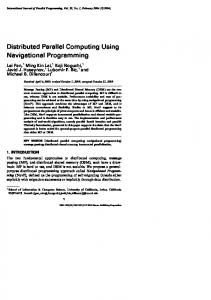
 Horizontal (Spatial) composition: A # B. Resulted program interface is: (west(A); north(A) ∪ north(B); east(B); south(A) ∪ south(B))

A

B

Fig. 3. Horizontal Composition. East(A) should match west(B).

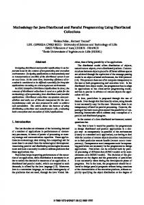
In [2], AGAPIA v0.1 was described as being a kernel programming language for interactive systems. It contains a detailed presentation of the language syntax and a toy example of dual-pass termination detection protocol. In [3], the syntax is extended to allow for the construction of high-level structured rv-programs. The new version of the language is v0.2 and supports recursion and dynamic programs creation. This paper is based on the latest version of AGAPIA, v0.2. To create high-level programs, AGAPIA provides composition operators, conditional and iteration statements. B. Basics of AGAPIA programming The basic block in AGAPIA programming is the module. A module has four input/output interfaces. The input can be received in north and west while output could go to east and south. Each interface could contain zero, one or more variables. A module’s interface could be represented as a tuple of interfaces: (west; north;east;south). The interface of the module in Fig. 1 is ( int,string ; nil ; int ; int). By specifying nil to an interface we are actually ignoring it. module main { listen a : int, s:string } { read nil } { // ..source code for program.. }{ speak b : int } { write c : int } North (read) input

nil a West input (listen)

b

main c

East output (speak)

South (write) output

Fig. 1. Simple program in AGAPIA.

To obtain higher-level programs, the basic operation for the user is to use the composition operators. In the pictures below all the three composition operators that can be defined over two programs A and B are shown, along with the necessary restrictions and resulted interfaces.

 Diagonal composition: A $ B. Resulted program interface is: (west(A); north(A); east(B), south(B)).

A B Fig. 4. Diagonal composition. Both output interfaces of A should match the input interfaces of B.

Two types of dependencies can be defined between modules:  north-south (or read-write) dependency: can occur in the vertical or diagonal composition.  east-west (listen-speak) dependency: can occur in the horizontal or diagonal compositions. A dependency exists if the interface on the corresponding side is not nil. Dependencies are usefully when coordinating the execution and preventing a program being executed before another one. For example, the diagonal composition could have both types of dependencies and it can be usefully when implementing barriers. The modularity of the language is given by the fact that a module implementation can be re-used in another application just by matching the correct interfaces. Also, at any time a user can change a module implementation with another one with the same interfaces. Making a comparison to general object oriented languages, a module change is like replacing an existing class with another one which have the same operations and data. However this is even easier in AGAPIA because the only specification of a module is contained in its input/output interfaces, while the entire semantics is contained inside the module. The original syntax of AGAPIA v0.2 language was modified in order to make it friendlier to users. In Fig. 5 the new syntax is presented. As the syntax is defined, a module becomes a program at a higher-level.

 Vertical (Temporal) composition: A%B. Resulted program interface is: (west(A) ∪ west(B); north(A); east(A) ∪ east(B); south(B)).

A

Interfaces SI ::= nil | int | bool | float | string | buffer | | (SI, SI) | (SI [] ) MI ::= (SI) | (SI;SI) | (SI;)* Expressions V ::= x : MI | V(k) | V.k | V.[k] | V@k | V@[k]

B

E ::= n | V | E + E | E * E | E – E | E/E

Fig. 2. Vertical composition. South(A) should match North(B)

B ::= b | V | B&&B | B || B | !B | E < E

34 | P a g e www.ijacsa.thesai.org

(IJACSA) International Journal of Advanced Computer Science and Applications, Vol. 5, No. 3, 2014

Programs W ::= null | new x : SI | x := E | if (B) { W } else { W } | W;W | while (B) { W } … (and all other C language constructs) M ::= module module_name [MI – optional]{listen x:MI}{read x:MI} { W } {speak x : MI}{write x : MI} P::= nil | M | if (B) { P } else { P } |P%P|P#P|P$P | while_t (B) {P} | while_s(B) {P} | while_st(B) {P} | gather(int) | scatter(int) | map(int,P) | reduce(int,P,P) | scan(int,P,P)

the array will go in the right order to M, N and Z. It is best to use array of processes when dealing with AGAPIA high level iterative statements ( for/each/while or patterns). In the case of the above example with M # N # Z then it suffices, and it is even clear, to have a spatial input like ( (bool,int) ; (bool, int) ; (bool, int)) – three process inputs, one for each program. C. High level statements To change the input/output flow by conditional branching, we can use the “if” program. It has the following syntax: if (condition) {P_IF } else { P_ELSE } , where P_IF and P_ELSE are also two programs. There are two restrictions regarding these two programs: P_IF and P_ELSE programs should have the same interfaces (and even input interfaces with the same variable names) to make the input/output matching correctly. “condition” can only contain variables defined in the input interfaces of P_IF and P_ELSE. Fig. 6 shows how an “if” program looks like inside. Inputs received are buffered until condition can be evaluated. north input condition evaluate over input

Fig. 5. The modified syntax of AGAPIA programs.

To be more appropriate to common programming languages some changes were done when writing AGAPIA code. “SI” from the syntax figure represents a simple interface declaration. Structures can be obtained by adding together more simple data types: (SI, SI). ( SI[] ) represents an array of simple data types. Instead of using sn/tn or sb/tb the decision was to merge them and use just int and bool for both temporal and spatial interfaces, but without losing the information of which category they are. Two new basic data types, “string” and “buffer” types were added for storing strings and sending buffers between distributed programs in an easy way. “MI” is used for defining a module interface and it basically uses “SI” for this. From (or in) a module interface, the output (or input) can flow to one or more other modules. (SI;SI) represents two different processes while (SI;)* is an array of processes. For example, if we are vertically composing a module M with a foreach_s statement, then the south output interface of M should be something of type (SI;)*. In basic AGAPIA programs users can use all type of C\C++ language constructs. At the high-level programs section, the language offers simple and high level composition and flow branching statements. The “for each” and patterns “gather”, “scatter”, “map”, “reduce”, “scan” were added in order to improve the expresivness. Because array of processes are something AGAPIA specific, some more details must be given. A simple array of structures (named A) of a pair containing an int and a bool is defined as A:(int, bool)[], while A[i] is used to access an index from this array. An array of processes (named V), with each process containing the same pair is defined as V:(int, bool;)*, while V@[i] is used to access an index. The main difference is that elements from a simple array can’t be split to different AGAPIA programs just by composition, while the array of processes can. If there is a program which has as spatial input an array of processes and inside this program there is a composition like M # N # Z, each one accepting a simple pair of int and bool as spatial input, then the first three indices from

West input

P_IF

East output

OR P_ELSE

south output

Fig. 6. Inside an if program in AGAPIA.

To create iterating compositions of programs, AGAPIA provides the following statements: for’s, fort, for_st, foreach_s, foreach_t, foreach_st, whiles, while_t, while_st. These are doing the same things as the “for” and “while” statements in the common programming languages, excepting that for each iteration an AGAPIA program is spawned and composed with other programs. Between consecutive iterations, the programs can be composed spatial, temporal and diagonal – as the usual programs composition. The type of the composition is indicated by the letters that comes after underscore in the statement name: “s” means spatial (#), “t” temporal (%), and “st” diagonal ($). This rule is valid for all types of “for/each/_” and “while_” statements. As we can see from the syntax, these statements become AGAPIA programs too. Fig. 7, 8, 9 shows how the for, foreach and while programs look internally for each iteration type. The figures are conclusive about how the input/output flows inside. north input …….

West input

…

East output

…….

south output

Fig. 7. Inside an for_s/foreach_s/while_s program. There is a spatial composition between consecutive iterating programs.

35 | P a g e www.ijacsa.thesai.org

(IJACSA) International Journal of Advanced Computer Science and Applications, Vol. 5, No. 3, 2014 north input

West input

. . .

. . . . .

. . .

East output

…..

south output

Fig. 8. Inside an for/each_t or while_t program. There is a temporal composition between consecutive iterating programs. north input West input

. . . . .

………………...

East output south output

Fig. 9. Inside an for_st/foreach_st or while_st program. There is a diagonal composition between consecutive iterating programs.

As with the “if” program condition, the “while_” program condition refers to the interface of the program it is iterating on. So if we have a program like while_t(condition) {P}, then condition can refer to the north and west input interfaces of P. If user knows the number of iterations then it is better in terms of performance to use the for/for each statements, because in background all internal instances could be created directly allowing the maximization of parallelism. There is one big difference between “for_” and “for each_”. “for_” should be used when we want to impose a certain order on how the internal programs are instantiated. If we have a program like foreach_s(n) {P}, and n value does not depend on the input/output of P, and P doesn’t have any listen-speak dependency, then those n instances of type P could be spawned and executed in parallel in any order. If we use for_s instead, then the internal instances will be instantiated in the order of the iteration (although they could also run in parallel, if there is no listen-speak dependency between them). Speaking in terms of interfaces, the iterating side of these programs has as interface an array of processes. If the interface of P is (west; north; east; south), then the for_s / foreach_s/while_s interface is (west, (north;)*, east, (south;)*). Some clarifications must be made about how the parameters containing arrays of processes are sent between programs. If the program which sends input for an array of processes is an atomic program, then all data is sent in a chunk. Same thing happens if the receiver program is a atomic (we achieve this by buffering the inputs and detecting when all input expected arrived). If none of the modules are atomic, and both programs are connecting an (int;)* to an (int;)* then the mapping is made on the same indices, 1:1. If not, and for example the array of processes has type (int;)*, then the input for this array of processes can contain in its specification just a single array of processes and this should be the last element. A

correct example is connecting (int;)* to (int ; int ;……;(int;)*. Connecting (int; (int;)*; int; …) to (int;)* is not allowed, because there is no mechanism to know how much the second item in the specification will expand. Considering these recursively, the compiler knows exactly the order of how elements come in the array. Also, for optimization purposes, if communicating programs are not atomic then we send array indices individually. Imagine a program which does some parallel computations and set individual items in an array of processes in the south interface. If this program is vertically composed with a foreach_s statement then sending array indices individually is a performance advantage. Each time an item is sent to the foreach_s program a new instance inside of it can start, maximizing this way the potential parallelism. The other high level statements, which represents some ready to use common patterns, were created in order to improve the productivity in building complex applications. Scatter is used to transform from a simple array to an array of processes while Gather transforms an array of processes to a simple array. Common usage examples can includes creating an array of tasks then splitting each item to a different program instance or receiving results from different programs in a simple array. The Map pattern can be used to apply an operation (represented by a given module) over a set of items and produce another set of items. Examples of usage include image processing, ray tracing or Monte Carlo sampling. AGAPIA also provides Scan and Reduce primitives which does the typical operations in logarithmic time over a set if inputs coming from different programs. Other kind of patterns such as pipeline or wavefront can be easily expressed just by using composition operators. D. AGAPIA runtime, backend and how to use interface variables. Paper [2] states in the „Conclusion and future work” section that we need an AGAPIA compiler. Because of this, the previous papers didn't talk about how the programs are being executed or the input/output flow in detail. The compiler is now publicly available at http://code.google.com/p/agapiaprogramming-language and it is continuously updated. A briefly presentation is made here about how the programs execution works. All programs looks like a dataflow graph with nodes representing smaller programs. The communication between these nodes is transparent, composition operators or high-level statements and patterns automatically creates in background the links between input/output interfaces. The source code for user written programs can be a mix of C\C++ and specific AGAPIA statements and operators. A program which doesn’t contain any specific AGAPIA composition or statements is called atomic. The semantic difference between the atomic programs and non-atomic ones is that the first category needs all the inputs available before starting to execute. The real computational tasks that can be executed in parallel by the internal schedulers are to be found in the atomic programs. To minimize the computational overhead, the atomic programs are translated and linked into C/C++ code. Only the non-atomic programs are being interpreted.

36 | P a g e www.ijacsa.thesai.org

(IJACSA) International Journal of Advanced Computer Science and Applications, Vol. 5, No. 3, 2014

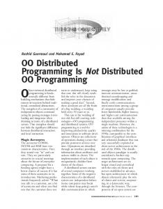
The scheduler is built on the top of MPI. The default scheduler’s architecture is composed by a master and multiple workers. The master process responsibility is to coordinate input/output of the modules and detect new atomic modules that can be executed. These atomic programs are executed as soon as there is an idle worker available. Users can change this default execution by using some specifier near a module definition. Specifier “@Master” can make a module to be executed only on master – this is typically useful when there is a resource available just on the master. A module can be executed and coordinated by the same worker by specifying “@SameProcess” – this behavior can reduce the transfer time or allow the usage of small coordination modules with minimal overhead. An important preparation for the next section is to show how we can use the variables defined in the interface of a program. The code below shows some examples of accessing input/output variables. We can access each one directly by its name. Usually we read from input interfaces, compute, then write in the output variables. Even if the below module has operator “@” used to access an array of processes, it still remains an atomic one and it is executed purely as C\C++ code. A parser included in the AGAPIA distribution translates in background the “@” operator into a series of C language calls. Module TEST {listen arrayOfProcesses : (int;)* } { read nil } { // Read a value from index 0 in an array of processes value = arrayOfProcesses@[0] ; // Set a value to a simple array index chrs[0] = ‘a’; }{speak chrs: char[] } {write value : int } III. PARALLEL PATTERNS IN AGAPIA This section presents some basic parallel programming patterns and how to implement them in AGAPIA. As Section 1 states, the patterns implemented here can be used in both shared and distributed memory models. A. Fork-Join The Fork-Join pattern lets control flow fork into multiple parallel flows that rejoin later [1]. It is the base of many patterns and its main usage is to split a process (parent) into two or more parts that could be computed in parallel. Below is an example of a simple implementation of this pattern in AGAPIA. A

from both programs A and B to continue execution. Both programs can be executed in parallel and having the listenspeak dependency between A and B guarantees that A start before B. The easiness of the implementation comes from the fact that the user just needs to write the correct interfaces for programs and use the composition operators. module ForkExample {listen nil}{read nil} { A#B % Join }{speak nil}{write nil} module A{listen nil}{read nil} { .. code ..} {speakta:int}{write sa:int} module B{listen ta:int}{read nil} { .. code ..} {speak nil}{write ba:int} module Join{listen nil}{read sa:int,sc:int} { .. code ..} {speak nil}{write nil} Creating a fork-join in MPI is possible by using the MPI_Comm_Spawn function. But there are some disadvantages over the AGAPIA solution. First thing is that user has to write different code/executable for the parent and child process. Then, communication between spawned child and joining is more complicated than in AGAPIA – user have to be carefully about calling MPI_Wait and MPI_Finalize in the right places and use the correct communication channel and id. B. Map The map pattern replicates a function over every element of an index set. The set can be abstract or associated with the elements of a collection [1]. Usually, it produces a new set of values, like in Fig. 11. Using this pattern user can write programs to solve problems like image processing, Monte Carlo sampling or ray tracing, in a parallel environment.

B

Join

Fig. 10. Example of a Fork-Join. The process that execute program A spawns a new process that execute program B, continues execution in parallel, and after some time they join.

By simple composition of programs we can create a ForkJoin pattern in AGAPIA. Because of the read-write dependency, the program Join knows that it needs to get input

Fig. 11. Map pattern example. The input is a set of values, it applies the same function over all items in the set and usually obtain another set of values.

A Map can be defined by hand if complex situation needs. To exemplify this and show the background implementation of

37 | P a g e www.ijacsa.thesai.org

(IJACSA) International Journal of Advanced Computer Science and Applications, Vol. 5, No. 3, 2014

a Map, an implementation in AGAPIA of this pattern is presented below. In this case the set is an array of processes of numeric values. A simple elemental function (the function being replicated) is used: multiply each number by two. module MapExample{listen n : int }{read inputs:(int;)*) } {

needs to run the elemental function. Also, for the two operations to complete, the root and workers should call them in the correct order. These disadvantages make this pattern implementation in MPI a slightly more error prone and harder to understand that it is by using AGAPIA which provides a clearer picture for users. C. Gather and Scatter The Gather pattern reads values from a set of processes and stores them in a collection. The Scatter pattern is the inverse of the Gather pattern – the values from a collection are distributed to multiple processes. These are base operations for parallel programming with distributed memory and are also implemented in MPI: MPI_Gather and MPI_Scatter. Below are both operations implemented in AGAPIA.

foreach_s(n) { ElementalFunc } }{speak nil}{write outputs:(int;)*)} module ElementalFunc{listen nil}{read in:int} { out = in*2; }{speak nil}{write out:int}

Fig. 12. Gather example.

The first n elements from “inputs” will get through the ElementalFunc, get multiplied by two, and then goes to the correct index in the “outputs” array. Because there is no listenspeak dependency, all ElementalFunc tasks can be executed in parallel. Compiler knows how to send the correct inputs from array to each ElementalFunc because, as Section 2 states, the elements in the “inputs” array will be available in the order the came in. Then, each input received will be sent to the correct iteration of the for each loop. If a needed input is not available yet in the array, the corresponding ElementalFunc instance will wait until it becomes available. AGAPIA provides an existing implementation of this pattern that users can use to simplify a program implementation. Users have to define what the map operations does on the input element with the correct input and output types in the interface and to give as parameter the number of items the map should apply to. Map automatically adjusts depending on the type of composition and data types. An example of usage where the map is applied over the output of n modules of type A, then results are used as input for n modules of type B is given below: foreach_s(n){A} % Map(ElementalFunc,n) % foreach_s(n){B}. To implement this in MPI we first need to send the input to different processes (either calling a Scatter operation, or using parallel I/O which were processes read data on their own). Then, these processes compute the desired operation - the elemental function - and finally, a gather operation will be used to copy the results back to a root process. As Scatter and Gather operations are implemented, we need to create another communication channel to contain just the processes that

module Gather{listen n : int}{read v:(int;)*} { for (int i = 0; i < n; i++) out[i] = v@[i]; } {speak n : int}{write out : int[]}

Fig. 13. Scatter example.

module Scatter{listen n : int}{read int: int[]} { for (int i = 0; i < n; i++) v@[i] = in[i]; }{speak n : int}{write v:(int;)*} Both patterns implementations are using the temporal interface for transmitting the number of items in the arrays. User could also choose to transmit the number of items through the spatial interface, but then he needs some identity operators to match correctly the interfaces. Examples can be found in [2] and [3]. AGAPIA already provides implementations for Gather and Scatter. A parameter representing how many items should be gathered/scattered must be given. An example to gather the results from a foreach_s statement in an array is: foreach_s(n) {A} % gather(n). This will gather the outputs from the south interface of all n modules of type A in a simple array. gather/scatter automatically define and checks the input/output interfaces depending on the source/destination of data. D. Pipeline The pipeline pattern is usefully when the computation involves performing a calculation on many sets of data and

38 | P a g e www.ijacsa.thesai.org

(IJACSA) International Journal of Advanced Computer Science and Applications, Vol. 5, No. 3, 2014

this calculation can be viewed in terms of data flowing through a sequence of stages. It is common in the implementation of real time applications, signal processing, online applications, compilers or systolic algorithms. There are two types of pipelines: linear pipelines – all stages that are applied over an input are executed serially, non-linear pipelines – can contain stages that could execute in parallel. Both types can be easily implemented in AGAPIA. Below is presented an implementation of a linear pipeline. input S1

S2

S3

S4

S1

S2

S3

S4

If we consider that a distributed system could run multiple non-linear pipelines in parallel then an implementation in MPI needs to use the dynamic process spawning or a custom scheduler created by user. The simplest way to do it, using dynamic process spawning, has some disadvantages. First, we need separate code files/executable for each component or group of components from pipeline that needs to be executed on different processes. This makes the code hard to follow, in contrast to AGAPIA where we have the entire code in one file, together with the entire pipeline flow. A second issue that appears often in pipeline applications is the diversity of parameters and data sent between components of the pipeline. In MPI we need several calls to MPI_Send and MPI_Recv functions. In AGAPIA the parameters are serialized and sent automatically according to programs interfaces.

………………………………………………...

Fig. 14. Linear pipeline. There are read-write dependencies between levels, and listen-speak dependencies for consecutive programs of a level.

module Pipeline {listen InImagesArray :(image;)*}{read nil} { for_t (int i = 0; i < NrImages; i++) { S1 # S2 # S3 # S4 } }{speak nil}{write OutImagesArray:(image;)*} We can make sure that a certain stage program can’t be executed in parallel on different levels by creating a write-read dependency. An example of this kind of behavior can be obtained for program S1 like this:

E. Geometric Decomposition The Geometric Decomposition pattern breaks data into a set of subcollections. The purpose is to give this data to different processes for parallel execution. Sometimes, it is not necessary to transfer the data, like in the case of programming for a shared memory model. Stencil operations, which are used in image processing and simulations, are good examples of usage for this pattern. Below is an example of an image filter skeleton implementation in AGAPIA which uses a shared memory model. The “Decomposition” program is responsible for breaking data – in our example it gives to each process, an equal number of consecutive lines from the input image. The number of tasks in which we want to break the computation of filter over the image is decided in this program by a call to an external function defined by user and transmitted through the temporal interface further. The “Task” program is the one responsible for executing the given part of the image. . . . . .

lineStart

module S1 {listen img: image}{read check:int}

Task index i

nrLines

{ .. code to compute the imgout..

Fig. 16. Image decomposition.

}{speak imgout:image}{write check:int} w, h, pixels []

We can even play with groups of dependencies between stages on the same level. It’s all about how the user put dependencies between programs. Non-linear pipelines can be easily obtained too:

Filter Decomposition Tasks[]

S2 S1

Computetasks

S4

nt

S3

for_s Task

Task

...... Task

Fig. 15. Non-linear pipeline. S2 and S3 can be executed in parallel.

A program with a pipeline like in Fig. 15 can be implemented by changing the source code inside the for_s statement from the previous pipeline implementation with: S1 # (S2%S3) #S4. By combining the pipelines with “if” statements, we can easily create some other kind of patterns like filters.

All Task modules can be executed in parallel.

Fig. 17. The flow of input and execution in AGAPIA. The programs are represented by rectangles and their name is in the top-left corner.

Module Filter{listen nil}{read w:int, h:int, pixels:int[]}

39 | P a g e www.ijacsa.thesai.org

(IJACSA) International Journal of Advanced Computer Science and Applications, Vol. 5, No. 3, 2014

{ Decomposition $ ComputeTasks }{speak nil}{write nil} module Decomposition{listen nil}{read w:int, h:int, pixels:int[]} { nt = Utils::GetNbOfTasks(w,h); for (int i = 0; i < nt; i++) {

Fig. 18. Tree reduction pattern for an associative combiner function.

The program Reduce receives as input an array of processes each one having an integer value. Inside, it uses a program CombineFunc which receives as input two integers values and outputs a single one – the value resulted by combining the inputs. A simple example of combine function could be the addition of numbers. module Reduce{listen nil}{read v:(int;)*) }

tasks@[i].lineStart= (h/nt) * i;

{

tasks@[i].nrLines= h/nt;

for_t (int i = 1; i