Distributed ray tracing for rendering voxelized LIDAR geospatial data Miha Lunar, Ciril Bohak, Matija Marolt University of Ljubljana Faculty of Computer and Information Science E-mail:
[email protected], {ciril.bohak, matija.marolt}@fri.uni-lj.si
Abstract In this paper, we present a distributed ray tracing system for rendering voxelized LIDAR geospatial data. The system takes LIDAR or other voxel data of a broad region as an input from a remote dataset, prepares the data for faster access by caching it in a local database, and serves the data through a voxel server to the rendering client, which can use multiple nodes for faster distributed rendering of the final image. In the work, we evaluate the system according to different parameter values, we present the computing time distribution between different parts of the system and present the system output results. We also present possible future extensions and improvements.
1
Introduction
People often desire a different view of the world, either for scientific or business needs or from just plain curiosity. In reality, viewing a location from vastly different vantage points can take a lot of effort, money and/or time. With aerial photography, and more recently laser scanning technology, being increasingly utilized across vast terrain or even entire countries, computer based rendering techniques are often employed to provide a relatively quick and cheap survey or visual representation of collected geospatial data. Rendering of volumetric voxel1 data is a problem with many existing solutions, including isosurface extraction through marching cubes [4], splatting [6] and voxel ray casting. Ray tracing, an extension of ray casting, is a rendering technique with extensive prior work on various methods and techniques [5]. Such visualization techniques are not available in commonly used GIS software (e.g. ESRI, Google Maps etc.). Geospatial science is a wide field of research and geographic information systems are often used in environmental agencies, businesses, and other entities. Countries are increasingly funding and openly releasing orthophoto imagery and laser scans of their terrain, making way for novel uses of their data. Our goal is to use such data for non-real-time rendering of the landscape in Minecraft-like visualizations. 1 A voxel in a voxel grid is the three-dimensional equivalent to a pixel in a 2D image.
2
System Architecture
The presented system is divided into two stages: preparation and rendering. An overview of the system architecture is shown in Figure 1. We use two data sources to prepare our operating data set: LIDAR2 squares, which are point clouds obtained from airborne laser scanning divided into 1 km2 squares on a 2D horizontal grid spanning across the country and aerial orthophoto images. In the first preparation stage we download and process LIDAR squares and orthophoto images using the “Resource Grabber” script written for the Node.js3 platform. The script reads a local database called Fishnet, which contains the definitions of all LIDAR squares and downloads the ones defined in preconfigured ranges from ARSO4 servers. After downloading the original zLAS5 formatted LIDAR squares, we convert them into the open LAZ 6 format for easier processing. The script is based on asynchronous queues and can download and convert multiple resources at once. In the rendering second stage, we use the ray tracer program to interactively render requested scenes. The ray tracer requires world data in a specific voxel format. We developed an HTTP voxel server to convert and cache prepared GIS data7 to boxes of voxels, which are then sent to the ray tracer on demand. Preparation LIDAR Data
Orthophoto
Resource Grabber
Rendering Ray Tracer
Configuration Fishnet Database
Voxel Server
Prepared GIS Data
Figure 1: System architecture diagram. 2 Light
Detection And Ranging. by the Node.js Foundation: https://nodejs.org/ 4 Slovenian Environment Agency. 5 ESRI proprietary compressed LIDAR file format. 6 Open compressed LIDAR file format. 7 Geographic Information System data. 3 Node.js
Ray Tracer
ZIP File
In our system, we use standard ray tracing techniques as described in [5], specifically shadow rays, reflection and refraction rays, ambient occlusion rays and aerial perspective. We developed the ray tracer specifically for walking through voxel fields. The first step in voxel traversal is quantization, where the initial point of the ray is converted into coordinates in the voxel grid. The algorithm presented in [1] then shows a way to step through voxels that the ray touches without missing corner cases or visiting the same voxel multiple times. In Section 3.1 we show how the main program splits up the desired image into pieces and sends them to available processors, then in Section 3.2 we show how a single processor loads and caches voxel worlds for ray tracing. 3.1 Rendering Architecture In Figure 2 we provide an overview of how the renderer selects which pixels to render and where. We also give a brief overview of what every part of this system does and why it is useful. Renderer
Multiresolution System
Distributed Processing Green
Worker
Tile
Scaled Image Tile System
Socket
Figure 2: Ray tracer rendering overview. We developed a multiresolution rendering system with lower resolution images being rendered first, which is useful for faster preview. The renderer then renders an image at double resolution until the requested target resolution is achieved. Since the difference is always a factor of 2, the results of a lower resolution render can be reused for a higher resolution render, with only the remaining 3 pixels rendered as depicted in Figure 3. Each scaled image is then split up into tiles of a predetermined size. This is good for cache locality because rays close together in space will be traced close together in time. We implement two tile orderings, a spiral one and a vertical one. The spiral ordering is better for interactivity, as it first renders the center of the image, which is usually the most useful while configuring parameters. The vertical tile order is better for cache locality with a mostly horizontal world. Splitting up the image into tiles additionally helps with the next step of dividing up the work among several possible processors.
Figure 3: Four resolution levels are shown as four shades of gray on a final 16 × 16 image. Higher resolutions are represented with brighter pixels.
Directory
Voxel Server Worker
Raw
Region
Anvil
Generated Socket HTTP
Remote
3
Box Cache Hash Table
Local Box
Block Manager Interface
Figure 4: Ray tracer world loading and caching. We send each tile to one of the available ray processors based on ray tracer settings. We implement three types. A green ray processor is implemented through the use of green threading, that is, the rays are processed for a certain chunk of time on the main thread before allowing for other processing to continue. Since this restricts the rendering to a single thread, we also implement worker and socket processors. A socket processor operates over TCP sockets and can run either as a separate program on the same computer, a different computer on the same network or even over the Internet. For worker and socket processors we also package and send the required state over the worker channel or network connection on demand. 3.2 World Loading and Caching Architecture To trace a voxel grid we first need to load a dataset that contains the voxels we wish to trace. We present an overview of the world loading architecture in Figure 4. We implement loading of three different world formats from the Minecraft video game, as that is a readily available source of large amounts of voxel data. These formats (Raw, Region, Anvil) can also be converted into a custom box format, similar to the ones used in Minecraft. For rendering in limited environments without external data sources, we implement a generated world type based on Simplex noise [3]. We also implement an HTTP voxel server which can convert LIDAR point clouds to a grid of voxels and serialize them into the mentioned custom box format, described in more detail in Section 4. All of the formats share the same basic idea – that the world is split up into chunks or vertical slabs of voxel data in a horizontal 2D grid. This allows for out-of-core processing of the world, as chunks can be loaded in and out of memory on demand. Loaded boxes are kept in a spatial hash table, using the Morton code [2] of their coordinates as the hash value for better hash locality. We developed the Block Manager to abstract all the world loading, caching and voxel access. Using the domain knowledge of the flat horizontal 2D chunk grid mostly filled with smooth terrain, we apply some specific accelerations to speed up tracing. If a ray is above or below the extents of the chunk grid, we first
advance the ray in its direction to the world data boundary. More granularly, we also advance the ray towards the bounding volume defined by the precomputed highest non-air voxel and the chunk walls.
4
Voxel Server
For the purposes of converting large amounts of LIDAR points into voxel data we developed a custom multithreaded HTTP server based on the CivetWeb8 web server library. Based on the position and size requested from the ray tracer, the server uses appropriate LIDAR squares to generate a chunk of voxel data in the form of a box, which it then sends back to the ray tracer. In the next sections, we describe a series of steps we used to convert points from the original point cloud format to a cleaned up voxel representation. 4.1 Box Cache In the case of distributed ray tracing, many clients can request the same boxes, so we implemented a box cache. It is similar to the ray tracer box cache, where the request is first checked against a spatial hash table and if available, the saved box is reused, otherwise, a new one is generated and stored in the cache. This greatly improves the server throughput in cases of simultaneous same box requests. 4.2 Point Loading In the first step of building a box, we load the requested range of points from one or more neighboring LIDAR squares. We use an area-of-interest rectangle query provided by the LASlib9 library to decompress and load the needed points into memory. Since we often need access to the same LIDAR squares from multiple threads, we use a pool of point readers to allow for simultaneous reading. 4.3 Quantization The list of loaded points resides in the ETRS8910 coordinate system, so we transform it into the box coordinate system and quantize the coordinates to integer values that a voxel can take. We store the classification of the loaded point into its place in the voxel grid. 4.4 Acceleration Structure Initialization We prepare two acceleration structures for easier and faster nearest point and column height queries later on. We use the nanoflann11 library to build a k-d tree of all the loaded points and separately of all the ground points, which enables fast nearest neighbor queries used in the next steps. We also compute the highest non-air voxel and the highest voxel classified as ground for all the vertical columns in the box and the box as a whole. 8 CivetWeb by The CivetWeb developers: https://github. com/civetweb/civetweb 9 LASlib (with LASzip) is a C++ API for reading / writing LIDAR by rapidlasso GmbH: https://github.com/LAStools/ LAStools/tree/master/LASlib. 10 European Terrestrial Reference System 1989. 11 nanoflann by M. Muja, D. G. Lowe and J. L. Blanco: https: //github.com/jlblancoc/nanoflann
4.5 Building Fill Buildings are represented in the source LIDAR data as mostly just roofs without any walls. We make the assumption that walls of buildings are mostly vertically flat, so we convert the classification of all the voxels underneath roofs to the “building” type down to the lowest voxel height in the box. 4.6 Ground Fill LIDAR points don’t cover the ground evenly due to laser scanning imperfections, additionally, they are defined only on the surface. For every computed ground column larger than 0 we assume that it has a defined height. For zero height ground columns, we approximate the nearest height from neighboring ground points. All the voxels underneath the ground column height are set to the classification of ground, filling all the holes and empty voxels underground. 4.7 Specialization The original LIDAR point classification types are limited, but fairly reliable. For a more realistic rendering, we specialize the topmost box voxels through the use of orthophoto imagery. We transform the voxel coordinates into ETRS89 to look up corresponding orthophoto pixel color values. We set up a color classification map and filled it with hand-picked color values from a selected orthophoto places and the classifications they represent. We map each looked up color value to a classification by simply finding the shortest Euclidean distance to the color in color map in RGB color space. 4.8 Water Equalization and Deepening Water is only classified in the specialization step, so it can be very noisy and unrealistic in places, especially near river banks and shores. We assume a single water level in a box, which we get from the median height of all the water blocks in the box. All the water blocks are then set to this equalized water level. Due to the nature of specialization, water is defined only on the surface. We artificially deepen it based on distance from shore.
5
Parameter Analysis and Results
We tested the system on an Intel Core i7 5820K 6-core processor running at 3.4 GHz, 32 GiB of system RAM running at 2400 MHz and a Samsung SSD 850 Pro 512GB solid state drive. We set the camera to a ≈500 m high bird’s eye view of Ljubljana with a 40◦ field of view. We used a memory limit of 700 MiB per ray tracer and a box size of 64 × 256 × 64. Viewpoints that are farther away demand more resources due to the amount of data and cache locality. The selected view is mid-ranged and the boxes it contains do not fit inside the 700 MiB memory limit. Figure 5 shows a couple of possible renders using our system. 5.1 Box Size We tested several different box sizes and recorded their rendering time.
Green 1 socket 6 sockets
2 workers 2 sockets 12 sockets
600 MiB/1200 MiB
300 MiB/900 MiB 30 20 10 0 30 20 10 0
Render Time [s]
Figure 5: Bled Island rendered using our system.
150 100 50
5
7
9
2468 1
3
5
7
9
2468
Interactive
of work done every second. Figure 9 shows the average step execution time for a single box.
Optimal 24 25 26 27 28
Combined Box Gen. Point Cloud Load Combined Filters Filter for Water Serialization Specialization Combined Ground Fill Iterative Ground Search Box Transmission k-d Build for All Filter for Asphalt Filter for Flat Roofs Filter with Null Target Filter for Orange Roofs Filter for Gray Roofs Transformation k-d Build for Ground Underground Fill Quantization Column Init. Building Fill Orthophoto Load LASlib Reader Init. Water Equalization Water Deepening
Figure 6: Rendering time versus box size, the most optimal box size was 64 × 256 × 64. Interactive means spiral tile order and several resolution levels, optimal means vertical tile order and the final resolution only. 5.2 Tile Size We also tested a range of different tile sizes with a hot and cold box cache. The optimal tile size in terms of processing speed was 50% of image height, however, for best interactivity, the best compromise was ≈ 15% of image height or ≈ 100px. Render Time [s]
3
80 60 40 20 0 80 60 40 20 0
Figure 8: Rendering time in seconds using different processor types over 10 runs.
Box Size [x × 256 × x]
100 80 60 40 20
1
4 sockets 12 HQ sockets
1 510 20 30 40 50 60 70 80 90 100 %
66 ms 36 ms 33 ms 19 ms 16 ms 14 ms 10 ms 7 ms 7 ms 6 ms 6 ms 5 ms 5 ms 4 ms 3 ms 2 ms 1 ms 882 µs 862 µs 167 µs 48 µs 39 µs 10 µs
0
283 ms
250 ms
435 ms
0.5 s
Figure 9: Average step execution time in voxel server box generation. 7.2 72 144
288
432
576
720 px
Tile Size [% of Image Height, x × x ] Cold Cache
Hot Cache
Figure 7: Render time of a 1280×720 image as a function of tile size in pixels and percent of image height.
5.3 Processor Type and Cache We tested the differently implemented processor types. Before each test, we cleared the box cache and then rendered the same scene 10 times, recording the render time after each run. This tests cache efficiency over time and runs. The results are displayed in Figure 8. 5.4 Voxel Server Step Timing We recorded the execution time of each step in the voxel server in a period of about half a minute. At the start, the server had an empty cache so as to avoid only recording execution time of the cache and network activity. Since the server is multithreaded, there can be multiple seconds
6
Conclusion and Future Work
We presented a novel system capable of rendering large amounts of LIDAR data on distributed machines. Our current implementation is suited for bird’s eye views, as we require all the boxes on a ray’s path to be loaded simultaneously. The voxel server we developed could be improved in many ways, however, we already get acceptable results for certain locations through the simple steps we have shown. Future work would also include a ray tracer capable of running across a variety of computing devices (e.g. GPUs) and more cache friendly ray sorting algorithms, which would speed up the rendering portion of the system. Rendering and point cloud data processing are both very wide fields of research, opening up a path to a multitude of new extensions, methods, improvements, and additions.
References [1]
J. Amanatides, A. Woo, et al. “A fast voxel traversal algorithm for ray tracing”. In: Eurographics. Vol. 87. 3. 1987, pp. 3–10.
[2]
S. E. Anderson. Bit Twiddling Hacks. 2009. URL: https://graphics.stanford.edu/˜seander/ bithacks.html#InterleaveBMN (visited on 07/02/2016).
[3]
S. Gustavson. “Simplex noise demystified”. In: Link¨oping University, Link¨oping, Sweden, Research Report (2005). URL : http : / / webstaff . itn . liu . se / ˜stegu / simplexnoise / simplexnoise . pdf (visited on 07/02/2016).
[4]
W. E. Lorensen and H. E. Cline. “Marching cubes: A high resolution 3D surface construction algorithm”. In: ACM siggraph computer graphics. Vol. 21. 4. ACM. 1987, pp. 163–169.
[5]
M. Pharr and G. Humphreys. Physically based rendering: From theory to implementation. Morgan Kaufmann, 2004.
[6]
L. A. Westover. “Splatting: a parallel, feed-forward volume rendering algorithm”. PhD thesis. University of North Carolina at Chapel Hill, 1991.