Distributed simulation of polychronous and plastic spiking neural ...

Distributed simulation of polychronous and plastic spiking neural networks: strong and weak scaling of a representative mini-application benchmark executed on a small-scale commodity cluster Pier Stanislao Paolucci1,*, Roberto Ammendola2, Andrea Biagioni1, Ottorino Frezza1, Francesca Lo Cicero1, Alessandro Lonardo1, Elena Pastorelli1, Francesco Simula1, Laura Tosoratto1, Piero Vicini1 1

INFN Roma “Sapienza”, Italy

2

INFN Roma “Tor Vergata”, Italy

*

Corresponding author: Pier Stanislao Paolucci, E-mail [email protected]

ABSTRACT We introduce a natively distributed mini-application benchmark representative of plastic spiking neural network simulators. It can be used to measure performances of existing computing platforms and to drive the development of future parallel/distributed computing systems dedicated to the simulation of plastic spiking networks. The mini-application is designed to generate identical spiking behaviors and network topologies over a varying number of processing nodes, simplifying the quantitative study of scalability on commodity and custom architectures. Here, we present a first set of strong and weak scaling measures of DPSNN-STDP benchmark (Distributed Simulation of Polychronous Spiking Neural Network with synaptic Spiking Timing Dependent Plasticity). In this first test, we used the benchmark to exercise a small scale cluster of commodity processors (varying the number of used physical cores from 1 to 128). The cluster was interconnected through a commodity network. Bidimensional grids of columns composed of Izhikevich neurons projected synapses locally and toward first, second and third neighboring columns. The size of the simulated network varied from 1.6 Giga synapses down to 200 K synapses. The miniapplication has been designed to be easily interfaced with standard and custom software and hardware communication interfaces. It has been designed from its foundation to be natively distributed and parallel, and should not pose major obstacles against distribution and parallelization on several platforms. During 2014, we will further enhance it to enable the description of larger networks, more complex connectomes, and prepare it for distribution to a larger community. The DPSNN-STDP mini-application benchmark is developed in the framework of the EURETILE FET FP7 European project.1 1. Introduction Brain simulation is: 1- a scientific grand-challenge; 2- a source of requirements and architectural inspiration for future parallel/distributed computing systems, 3- a parallel/distributed coding challenge. The main focus of several neural network simulation projects is the search for a)biological correctness; b)-flexibility in biological modeling; c)-scalability using commodity technology [e.g., NEURON (Carnevale, 2006, 2013); GENESIS (1988, 2013); NEST (Gewaltig, 2007);]. A second research line focuses more explicitly on computational challenges when running on commodity systems, with varying degrees of association to specific platforms echo-systems [e.g., Del Giudice, 2000; Modha, 2011; Izhikevich, 2008, Nageswaran, 2009]. An alternative research pathway is the development of specialized hardware, with varying degrees of flexibility allowed [e.g. SPINNAKER (Furber, 2012), SyNAPSE or BlueBrain projects]xs. Since 1984, the focus of our APE lab at INFN is the design and deployment of parallel/distributed architectures

1

The EURETILE project is funded by the European Commission, through the Grant Agreement no. 247846, Call: FP7ICT-2009-4 Objective FET-ICT-2009.8.1 Concurrent Tera-device Computing. See Paolucci et al, 2013.

1

dedicated to numerical simulations (e.g. Avico et al., 1986; Paolucci, 1995), and, it is now focusing on the development of custom interconnection networks (R Ammendola et al ., 2011). Indeed, the original purpose of the DPSNN-STDP project is the development of the simplest yet representative benchmark (i.e. a mini-application), to be used as a tool to characterize software and hardware architectures dedicated to neural simulations, and to drive the development of future generation simulation systems. Coded as a network of C++ processes, it is designed to be easily interfaced to both MPI and other (custom) Software/Hardware Communication Interfaces. It has been designed from its foundation to be natively distributed and parallel, and should not pose obstacles against distribution and parallelization on several competing platforms. It should capture major key features needed by large cortical simulation, and should serve the community of developers of dedicated computing systems or the tuning of commodity platforms. One of the explicit objectives is to maintain the code readable and its size at a minimum, to facilitate its usage as a benchmark. During 2014, we will further enhance it to enable the description of more complex connectomes, and other models and we will prepare it for a possible distribution to a larger community of users. This document presents a first set of strong and weak scaling measures of our DPSNN-STDP miniapplication benchmark, run on a small scale cluster of commodity processors interconnected through a commodity network. The “Methods” section of this document provides a compact description of the features of the October 2013 release of the DPSNN-STDP mini-application benchmark. The “Results” section reports the strong and weak scaling measures produced running the code on a small scale commodity cluster. We analyze the results in the “Discussion” and “Conclusions” section of the document. 2. Methods A complete technical report describing the internal structure of the October 2013 release of the DPSNN-STDP will be published before January 2014. Here, we provide a compact summary. The full neural system is described by a network of C++ processes equipped with a message passing interface. The full network is divided into clusters of neurons and their set of incoming synapses. Each synapse details the total transmission delay introduced by the axonal arborization that reaches it. Each cluster is simulated by a C++ process. The messages travelling between processes are sets of “axonal spikes” (i.e. they carry info about the identity of neurons that spiked and the original emission time of each spike). Axonal spikes are sent only toward those C++ processes where a target synapse exists. The sum between the original emission time of each spike and the transmission delay introduced by each synapse allows for the management of synaptic Spike Timing Dependent Plasticity and for the observation of phenomena related to difference among delays of individual synaptic arborizations (polychronism, see Izhikevich, 2006). There are two phases in a DPSNN-STDP simulation: 1- the initial construction of the system of neurons and the creation of the initial network of axonal polychronous arborizations and synapses that interconnect the system; 2- The dynamic phase. The dynamic phase can be further decomposed into four steps: 2.1- neurons follow their dynamic and can produce spikes; 2.2– Spikes reach target synapses through polychronous axonal arborizations; 2.3– Synapses inject currents into their target neuron; 2.4- Synapse evolve according to the polychronous STDP (Spiking Time Dependent Plasticity) (Song, 2000), which produces effects of Long Term synaptic Potentiation/Depression (LTP/LTD). We adopted a combined event-driven and time-driven approach (Morrison et al, 2005): • Event-driven simulation, for synaptic dynamics. • Time-driven simulation, for neural dynamics. Spiking neuron model Hybrid models describe the continuous evolution of several state variables (including a “membrane voltage” and auxiliary “currents”) and discrete events associated to the spiking event, i.e. special 2

rules applied to (a subset of) the state variables. Well known are the Hodgkin-Huxley (HH) (Huxley, 1952), the leaky integrate-and-fire (LIF) and the Izhikevich (IZH) (Izhikevich, 2003). For this experiment we adopted the IZH model which is computationally efficient (13 – 26 operations per simulated ms per neuron), and yet capable of replicating the spiking behaviour of several neuron types (Izhikevich, 2004).

𝒊𝒇  𝒗(𝒕) < 𝑣!"#$

𝑡ℎ𝑒𝑛

𝒊𝒇  𝒗(𝒕) ≥ 𝑣!"#$

𝑡ℎ𝑒𝑛

∆𝒗 = 𝒗(𝒕)𝟐 − 𝒖(𝒕) + 𝑰(𝒕) ∆𝒕 ∆𝒖 = 𝒂(𝒃𝒗(𝒕) − 𝒄) ∆𝒕   𝒗 𝒕 = 𝑣!"#$ 𝒗(𝒕 + ∆𝒕) ← 𝒄 𝒖(𝒕 + ∆𝒕) ← 𝒖(𝒕) + 𝒅

where: • v (t) is the neural membrane potential. This is the key observable; we say that when v reaches vpeak a “neural spike” happened; • I(t) is the potential change generated by the sum of all synapses incoming to the neuron. Incoming currents are present if spikes arrived form presynaptic neurons; • u(t) is an auxiliary variable (the recovery current bringing back v to equilibrium); • a, b, c, d are four parameters, constant for each neuron kind, by varying them the same equation model several kind of known neural types. In this experiment we used a mix of 80% excitatory RS Izhikevich neurons (i.e.: a=0.02, b=0.2, c = -65.0 mV, d=8.0) and 20% inhibitory FS neurons (obtained by setting a=0.1, b=0.2, c = -65.0 mV, d=2.0). vpeak was set at 30 mV. Synaptic update: spike timing dependent plasticity Let us define t = tpost – tpre – daxon, the time difference between the post-synaptic spike time, and the time of arrival of a spike originated by a presynaptic neuron at an original emission time tpre, that arrives at the target after an axonal delay daxon. We implemented the following STDP rule, to compute the ΔWpre,post change to the synaptic strength (Song et a., 2000). A+, A-, τ+, τ-, are parameters which permits to match the model on different types of neurons and biochemical contexts. 𝑡 = 𝑡!"#$ − 𝑡!"# − 𝑑!"#$      

𝑖𝑓    𝑡 ≥ 0 𝑖𝑓  𝑡 < 0    

!

∆𝑊!"#,!"#$ = 𝐴! 𝑒−!! !

∆𝑊!"#,!"#$ = 𝐴! 𝑒!!

The synapse is maximally potentiated if the delay introduced by the axon carries the signal to the target just before the post-synaptic spike (i.e. it is probably the cause of the spike). The synapse is maximally depressed if the signal arrives just late. Distributed generation of connection requests In our polychronous networks each neuron i = 1..N projects its set of forward synapses j=1..M, each one characterized by its individual delay D i,j, plastic weight W i,j and target neuron K i,j. In this set of tests, M was fixed to 200 for all neurons. Inhibitory neurons projected synapses only toward excitatory neurons located in the same column. Instead, excitatory neurons projected also to neighboring columns, as already discussed in a previous section. For this experiment, limited to a bidimensional grid of neural columns and a moderate number of synapses, we assigned delays in the range between 1 and 5 ms. Inhibitory synapses were assigned with the minimum delay, while excitatory delays were assigned with a uniform distribution of delays. If a neuron fires at a time ti, each forward synapse will have to inject a current W i,j at a synaptic specific time ti + D i,j. The 3

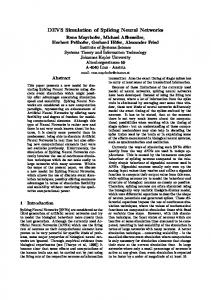
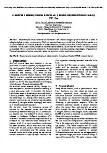
current W i,j will be injected in the target neuron kj=K i,j, where it will add to the currents arriving in the same time step from other source neurons, to form the total external incoming current Ik(t) which contributes to the dynamic of neuron kj. Bidimensional arrays of neural columns and their distribution on the processes and processors In this experiment of strong and weak scaling behavior, we arranged the neurons in “columns”, each one composed by one thousand neurons. Columns are then arranged in bidimensional grids (see Figure 2-1). Each excitatory neuron projected 76% of its synapses to neurons in its own column, 12% of its synapse toward neurons in first neighboring columns, 8% towards second neighbors and 4% toward neurons in third neighboring columns (see picture). Inhibitory neurons projected their synapses only towards excitatory neurons in the same column. We varied the total number of columns between one and 8192 (a 128x64 grid of neural columns). Each process can either host a fraction of a column (e.g. 1/8, ¼ …), a whole single column, or several columns (in the present version, up to 32 columns per process). When performing strong and weak scaling measures, periodic boundary conditions are used for columns at the boundary of the grids, to get more homogeneous spiking rates for different numbers of columns. For grids so small not to have enough distinct neighbors, the periodic boundary rule can end projecting more synapses on the same target column than expected for a large grid. Actually, in the case of a single column, all synapses are projected by the column to itself.

Figure 2-1. Example of distribution of an identical problem over a varying number of software processes and computational cores. In this figure, the grid to be distributed is composed by 8x8=64 neural columns. The DPSNNSTDP simulator produces the same external stimulus, synaptic structure and spiking activity on all distributions.

4

Distributed generation of reproducible connections and external “thalamic” stimulus We mention a feature that has been of some importance to simplify the execution of repeatable strong and weak scaling measures, while varying the number of processes and hardware resources (e.g. processors). We mean, the capability to initialize in a distributed manner an identical network and provide, again in a distributed manner, the same external “thalamic” stimulus to a network composed by a given grid of neural columns, distributed over a varying number of software processes and hardware processors. In a system with N total neurons, distributed among H software processes we can assign a fair share of locN = N/H neurons per software process, and the global and local identities of neurons can be easily computed using the local identifiers of processes and neurons. If there is a grid of CFT = CFX x CFY neural columns, and this info is known to each process, it will be easy for each process to generate autonomously forward connectivity patterns that does not depend on the number of processes/hardware processors. The same can be done to generate patterns of external “thalamic” stimulus to the network, e.g. prescribing the number of events per ms per neural column. Production of Observables The DPSNN-STDP code can produce files tracing several observables (list of individual spiking times and spiking neuron identity, mean spiking rates, membrane potentials, synaptic values). The code is equipped with facilities for distributed measurement of time spent on execution of individual routines and sections of the code based on the MPI_WTIME function.

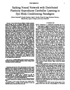
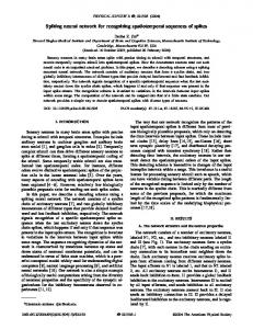
Figure 2-2. A sample trace of 320 ms of spiking activity, produced by the DPSNN-STDP code. In this case, it is the simulation of a single neural column, composed by 1000 neurons (80% excitatory RS, 20% inhibitory FS Izhikevich neurons). Above, each dot in the rastergram represents a spiking event. Below, the traces of the membrane potential of two excitatory neurons.

If necessary, the trace of the evolution of the membrane potential and other state variables of individual neurons can be activated. The membrane potential of a “resting” neuron fluctuates around a -70mV potential as a result of its own activities and of the perturbation produced by signals produced by other neurons. When the neuron decides to “fire”, its membrane potential (v state variable) starts to climb to positive voltages. If a “spike” happened, the Izhikevich rules drops the voltage down to its after spike potential, but the internal variable u keeps a memory of the past. This event is the “spike” of an individual neuron, which is propagated by the axon, and reaches a set of synapses after a time delay, 5

specific for each synapse, which depends on the distance travelled). When reached by the spike, each synapse produces a perturbation of the membrane potential of the target, which depend on its “strength” (here, we consider the simplistic case of the neural soma and dendritic arborization represented by a single “compartment”, i.e. a single u(t)-v(t) pair in the case of the Izhikevich equation). The following picture reports about 320 ms of collective spiking activity of a single column of 1000 neurons (800 RS excitatory, 200 FS inhibitory), and the evolution of the individual membrane potential of two neurons. In the “rastergram” the horizontal axis is the simulation time, the vertical axis the identifier of individual neurons. Each dot in the rastergram represents a spiking event. Representation of spiking messages Spiking messages are sent using an address event representation (AER): we send “axonal spike” messages that carry the identifiers of spiking neurons and are packed in groups that have the same spike emission time and the same target process (i.e. same target cluster of neurons). Our strategy is to defer as much as possible the arborization of the “axon”, to reduce the load on the network and unnecessary wait barrier (i.e. waiting for the completion of computations of cluster of neurons from which a process does not expect messages). To this purpose, we perform some preparatory actions during the network initialization phase (performed once at the beginning of the simulation), to reduce the number of active communication channels during the iterative simulation phase. Initial construction of the connectivity infrastructure During the initialization phase, each process can contribute to create the awareness about the subset of processes that should be listened to, during next simulation iterations. At the end of this construction phase, each “target” process should know about the subset of “source” processes that need to communicate with it, and should have created its database of locally incoming axons and synapses. A simple implementation of the construction phase can be realized using two steps. During the first step, each source process informs other processes about the existence of incoming axons and about the number of incoming synapses to be established. A single word, the synapse counter, is communicated among pairs of processes. Under MPI, this can be achieved by an MPI_Alltoall(). Performed once, and with a single word payload, the cost of this first step, creates a cumulative network load proportional to the square of the number of processes. The cost of this operation is negligible in the range of processes and synapsed explored by this paper. The second step transfers the identities of synapses to be created on each target process. Under MPI, the payload, a list of synapses specific for each pair in the subset of processes to be connected, can be transferred using a call to the MPI_alltoallv()library function. The cumulative load created by this second step is proportional to the product between the total number of processes and the subset of target processes reached by each source process. The first step produces two effects: 1- it reduces the cost of initial construction of synapses, second step of the construction phase; 2- the knowledge about the existence of a connection between a pair of processes can be reused to reduce the cost of spiking transmission during the simulation iterations. Delivery of spiking messages during the simulation phase Here, we describe the present implementation of the delivery of spiking messages. In this first implementation, we did not take advantage of the possibility of delivering spikes to targets just before the deadline imposed by the synaptic specific delay. Instead, we used a synchronous approach: all spikes are delivered to target processes before proceeding to the simulation of next time step of the neural dynamic. The delivery of spiking messages can be split in two steps, with communications directed toward subsets of decreasing sizes. During the first step, single word messages (spike counters) are sent to the subset of potentially connected target processes. On each pair of source-target process subset, the individual spike 6

counter informs about the actual payload (i.e. axonal spikes) that will have to be delivered, or about the absence of spikes to be transmitted between the pair. The knowledge of the subset has been created during the first step of the initialization phase, described in a previous section. The second step uses the spiking counter info to establish a communication channel only between pairs of processes that actually need to transfer an axonal spikes payload. On MPI, both steps can be implemented using calls to the MPI_Alltoallv() library function. However the two calls establish actual channels among sets of processes of decreasing size, as described just above. For the simple bidimensional grid of neural columns and for the mapping on processes used in this experiment this implementation demonstrated to be quite efficient, as reported by the measures presented in the “Results” section, further refined in the “Discussion” section. However, we expect that the delivery of spiking messages will be one of the key point still to be optimized for large scale simulations and when white area “connectomes” will be introduced, describing the communication channels among a multiplicity of remote cortical areas. 3. Results This section presents the strong and weak scaling behavior of the first revision (October 2013) of the DPSNN-STDP mini-app benchmark, run on a small scale commodity cluster. We run on a cluster of sixteen dual socket quad core servers, interconnected through a 40 Gb/s commodity network, for a maximum of 128 physical cores2. Each physical core supported two simultaneous threads. During this experiment, for each neural network size, we checked that the list of spiking neurons and their timings were identical for all run performed using a variable number of software processes and/or physical cores. For this measure, we varied the size of the network between a minimum of 200 K synapses and a maximum of 1.6 G synapses. Each network was distributed on a variable number of software processes, then assigned to a variable number of physical cores. Each MPI process hosted a maximum of 16 neural columns (i.e. 16 K neurons), and a minimum of 1/8 of neural column (i.e. 125 neurons). Due to the hardware support for two simultaneous threads per core, we observed that, in the majority of the cases, the best execution time was reached when two MPI software processes were launched on each physical core. Table 1. We run different problem sizes, from 200 K synapses to 1.6 billion synapses. Each network size, was distributed using a varying number of MPI processes, and run on a varying number of physical computational resources. Each problem size produced the same detailed firing activity, independently from the distribution. Synapses Neurons Grid of neural columns Firing rate (Hz) Used cores (min-max) MPI processes

200K 1K 1x1

3.2 M 16 K 4x4

6.4 M 32 K 8x4

12.8 M 64 K 8x8

25.6 M 128 K 16x8

51.2 M 256 K 16x16

102.4 M 512 K 32x16

0.4 G 2.0 M 64x32

0.8 G 4.1 M 64x64

1.6 G 8.0 M 128x64

20 1-8

26 1-64

29 2–64

31 4–64

33 8–128

33 8–128

40 32–128

43 32–128

36 64-128

48 128

1-8

1-128

2- 28

4–256

8- 28

16-256

32-256

128-256

256

256

We measured the execution time needed by the first 2000 steps of simulation of the spiking activity and synaptic plasticity. As expected, at the beginning of the simulation, the network exhibited high firing rates (in the range between 24 and 48 Hz). Indeed, the initial value of all excitatory and inhibitory synapses was set to a high strength, and during the first second of simulated activity the 2

Each server is a 1U SuperMicro X8DTG-D. Each node in the cluster is a dual socket. Each socket hosts one quad-core Intel(R) Xeon(R) CPU E5620 (max clock @ 2.40GHz). On each core HyperThreading is enabled (two threads per core). Each node is equipped with a Mellanox InfiniBand board, the MT26428 [ConnectX VPI PCIe 2.0 5GT/s - IB QDR (40Gb/s data rate)]. 16 nodes are connected using a Mellanox Switch.

7

STDP plasticity mechanism had not yet had enough time: 1- to select a subset of synapses, and 2- to bring the synaptic strength down to their distribution range. However, in the context of this measure, such an initial high activity was a desirable feature, because it translates into a high number of spiking messages to be distributed among the software processes and computational resources. Strong scaling The computational load needed to solve the simulation problem is expected to be proportional: a) to the number of simulated synapses, b) to the firing rate and c) to the physical time to be simulated.

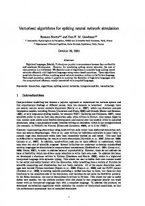
Figure 3-1. Strong scaling

Therefore, if we divided the measured execution time on a given number of computational cores by the product of a, b and c, we should obtain an estimate of the execution time needed per synapse per second. In first approximation, we could expect this number to be similar for different problem sizes. Then, an ideal code distributed on an ideal machine should half its execution time when doubling the number of computational cores assigned to the solution of the problem. Here below a picture of the scaling we observed running the DPSNN-STDP code. Surely, in Figure 3-1, we observe a scaling on the log-log graph, which, however, if far from be ideal. As the behavior is remarkably independent from the problem size, when normalized as described, let us discuss the measures of the 51.2 M synapse case. Instead of decreasing at each doubling in the number of cores of a factor 2, it decreases of an approximate factor 1.69 per doubling. Using this slope as representative, the multiplication of the number of cores by a factor 8

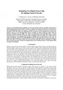
128 would decrease the simulation time by a factor 39 only, i.e. at least 3 times worst that an ideal scaling. We analyze the results in next “Discussion” section. Weak scaling If, instead of dividing the execution time by the total number of synapses, we divided it by the number of synapses assigned to each computational core, we should obtain, for the same consideration of the previous section, a value that for an ideal code, executing on an ideal machine should be constant for different network sizes and number of computational cores assigned to the solution of the problem. Figure 32 is the graph of our measures. Actually, the behavior for Figure 3-2. Weak Scaling different problem size is remarkably homogeneous. Therefore, let us use in the following the data measured on the 3.2 M synapse/core case as representative. On a single core the time needed to simulate one second of activity of each synapse, normalized by the firing rate, is 3.4 E-7 seconds, while it grows to 1.0 E-6 seconds when run on 128 nodes (a factor 2.9 of slow-down, compared to the ideal scaling case). We analyze the finding in the next “Discussion” section. 4. Discussion Searching for better scaling solutions At first sight, if one looked naively at the measures of time spent in the two step communication of spikes, one could derive a wrong conclusion: the non ideal scaling could be attributed to the cost of communications. On the contrary, in this case (a regular grid of neural columns connected to a few first neighbor neural columns), and for this synchronous implementation of the communication of spikes, additional measures discussed in this section appear to point to another cause: loadbalancing. The non-equal rate of activity between different portions of the network would force some processes to wait for others at each simulation step. If we were right, there should be a simple approach that should mitigate the case, distributing neurons of a single column among several processes After insertion of an explicit synchronization barrier, placed before the communication of spikes, we measured a set of times on each process, accumulated over the 2000 iterations of each run: 1the cumulative time spent by a process on the barrier itself, i.e. the time spent waiting for other processes completing their computations; 2- the cumulative time spent for the transmission/reception of the single word spike counter, that informs about the payload to be transmitted; this exchange happens with a few neighboring processes; 3- the cumulative time spent on axonal spiking payload transmission; on each channel, individual payloads are sent to further restricted subsets of neighboring processes, those containing targets for individual axonal spikes; 4the total elapsed time (equal for all processes). As we can notice, in Table 2., the sum of times 2) 9

and 3), the actual time spent on communication, is at most one tenth of the total time. The measurement did not cover the full range of cases explored by prvious sections, but the qualitative indication seems clear. Table 2. The time spent on the transmission of the spikes is never more than 10% of the total time. In this simple case, even if the network is evenly distributed among processes, each process spends a significant fraction of its time waiting for the completion of those processes where there is a greater computational activity. The role of “active” and “waiting” process changes over time. If we were right, this could be cured distributing neurons of a column among different computational resources.

Hardware  cores   MPI  processes   Neural  columns   1-­‐  barrier  (seconds)   2-­‐  spikes  dim  (s)   3-­‐  spikes  payload  (s)   Other  (s)   4-­‐  total  fire  (sec)  

8   16   2  

8   16   4  

8   16   8  

8   16   16  

8   16   32  

8   16   64  

8   16   128  

0,71   0,09   0,04   0,11   0,95  

1,77   0,13   0,15   0,24   2,29  

2,65   0,19   0,25   1,61   4,7  

2,79   0,47   0,27   4,29   7,82  

6,67   0,07   0,07   10,09   16,9  

13,40   0,15   0,35   26.00   39,90  

37,66   0,07   0,31   45,96   84,00  

5. Conclusions We introduced a natively distributed mini-application benchmark representative of plastic spiking neural network simulators. It can be used to measure performances of existing computing platforms and to drive the development of future parallel/distributed computing systems dedicated to the simulation of plastic spiking networks. The mini-application is designed to generate identical spiking behaviors and network topologies over a varying number of processing nodes, simplifying the quantitative study of scalability on commodity and custom architectures. Here, as a test case, we presented a first set of strong and weak scaling measures on a small scale cluster of commodity processors (varying the number of used physical cores and the problem size) and searched for the cause of the deviation from the ideal scaling behavior for a simple neural network structure (bidimensional grids of neural columns, connected to first, second and third neighboring columns). In this case, we indentified a possible strategy that could lead to a better scaling, that will be verified in a future work. More in general, our expectation is that the potential performance improvements from dedicated software and hardware co-design solutions will grow, when more complex interconnection topologies (e.g. inter-areal connectomes) will be simulated. The miniapplication has been designed to be easily interfaced with standard and custom software and hardware communication interfaces and permit easy measurements of scalability. It has been designed from its foundation to be natively distributed and parallel, and should not pose major obstacles against distribution and parallelization on several platforms. During 2014, we will further enhance it to enable the description of larger networks, more complex connectomes, and prepare it for distribution to a larger community. Meanwhile, the DPSNN-STDP mini-application benchmark will be validated against biologically significant cases. 6. Acknowledgements This work has been partially supported by the EURETILE European integrated FP7 project grant no. 247846. We also acknowledge the contribution of several valuable discussions with Paolo Del Giudice and Maurizio Mattia. 7. References N.T. Carnevale, M.L Hines. The NEURON Book. Cambridge University Press, (2006) N. T. Carnevale, M. L. Hines. NEURON for Empirically-Based Simulations of Neurons and Networks of Neurons. Available online at: http://www.neuron.yale.edu/neuron/. (retrieved October 2013)

10

J.M Bower, D. Beeman. The Book of GENESIS. Exploring realistic neural models with the GEneral NEural SImulation System (1988). GENESIS: GEneral NEural SImulation System. Available online at thhp://www.genesis-sim.org (retrieved Ocotber 2013) Gewaltig M-O & Diesmann M. (2007) NEST (Neural Simulation Tool) Scholarpedia 2(4):1430. P. Del Giudice, M. Mattia. Efficient Event-Driven Simulation of Large Networks of Spiking Neurons and Dynamical Synapses. Neural Computation, 12, 2305-2329 (2000). A. Morrison, C. Mehring, T. Geisel, A. Aertsen, M. Diesmann. Advancing the Boundaries of HighConnectivity Network Simulation with Distributed Computing. Neural Computation, 17, 1776-1801 (2005). S. B. Furber, D. R. Lester, L. A. Plana, J. D. Garside, E. Painkras, S. Temple, A. D. Brown. Overview of the SpiNNaker system architecture. IEEE Transactions on Computers, vol. PP, no.99, (2012). doi: 10.1109/TC.2012.142. Xin Jun, Steve B. Furber, John V. Woods. Efficient Modelling of Spiking Neural Networks on a Scalable Chip Multi-processor. Int. Joint Conf. on Neural Networks 2008 (IJCNN 2008), 2812-2819 (2008) . E. M. Izhikevich, G. M. Edelman. Large-scale model of mammalian thalamocortical systems. PNAS March 4, 2008 vol. 105 no. 93593-3598. Modha, S. D., & al., e. (2011). Cognitive Computing. Communications of the ACM , 54 (08 (pag. 62-71)). Jayram M. Nageswaran et al. (n.d.). Efficient Simulation of Large-Scale Spiking Neural Netwoks Using CUDA Graphics Processors. Int. Joint Conf. on Neural Networks 2009 (IJCNN 2009), 2145-2152 (2009). N. Avico et al. From APE to APE-100: from 1 to 100 Gigaflops in Lattice Gauge Theory Simulations. Comput. Phys. Commun. 57(1989)285. P.S. Paolucci. N-Body Classical Systems and Neural Networks on APE100 Massive Parallel Computers. Int. Journ. Mod. Phys. C 6(1995)169. Paolucci, P.S., Bacivarov, I., Goossens, G., Leupers, R., Rousseau, F., Schumacher, C., Thiele, L., Vicini, P., "EURETILE 2010-2012 summary: first three years of activity of the European Reference Tiled Experiment.", (2013), arXiv:1305.1459 [cs.DC] , http://arxiv.org/abs/1305.1459 R Ammendola et al . (2011). APEnet+: high bandwidth 3D torus direct network for petaflops scale commodity clusters. J. Phys.: Conf. Ser. 331 052029 doi:10.1088/1742-6596/331/5/052029 A.F.Huxley and A.L.Hodgkin. (n.d.). A quantitative description of membrane current and application to conduction and excitation in nerve. Journal of Physiology, 117, 500-544 (1952) . Izhikevich, E.M. Dynamical Systems in Neuroscience: the Geometry of Excitability and Bursting. Cambridge, MA: The MIT Press (2006). Izhikevich, E. M. Simple Model of Spiking Neurons. IEEE Transactions on Neural Networks, Vol. 14, No. 6, November 2003 . Izhikevich, E. M. Which Model to use for cortical spiking neurons? IEEE Transaction on Neural Networks, 15, no. 5 1063-1070 (2004) . C.C.Bell, et al. (n.d.). Synaptic plasticity in a cerebellum-like structure depends on temporal order. Nature 387, 278–281 (1997) . S. Song, K.D. Miller, L.F. Abbott. Competitive Hebbian learning through spike-timing-dependent synaptic plasticity. Nature Neuroscience 3, 919-926, (2000) . Izhikevich, E. M. Polychronization: Computation with Spikes. Neural Computation, 18, 245-282 (2006).

11