Department of Electrical and Computer Engineering. The University of ... Abstract. The traffic load of wireless local area networks (WLANs) is often dis- ... tree repair mechanism instead of complete pseudo-tree reconstruction when instability ...
DLB-SDPOP: A Multiagent Pseudo-tree Repair Algorithm for Load Balancing in WLANs Shanjun Cheng, Anita Raja Department of Software and Information Systems The University of North Carolina at Charlotte Charlotte, NC 28223 {scheng6, anraja}@uncc.edu
Abstract The traffic load of wireless local area networks (WLANs) is often distributed unevenly among access points. In addition, interference from collocated wireless devices operating in the same unlicensed frequency band may cause WLANs to become unstable, leading to temporary failures of access points. This paper addresses the questions of how to dynamically balance the load and how to quickly respond to instability in WLANs1 . We present a new decentralized multi-agent load balancing framework for WLANs that uses DLB-SDPOP, a distributed optimization algorithm, to dynamically load balance the WLAN. The algorithm implements a less expensive pseudotree repair mechanism instead of complete pseudo-tree reconstruction when instability problems occur. It also leverages an efficient communication mechanism to control communication overhead in heavily loaded situations. We empirically show that DLB-SDPOP improves WLAN load balancing performance significantly.
1. Introduction Wireless local area networks (WLANs) have become one of the most popular wireless technologies due to their low cost, simple installation, and great capability to support high speed data communications. However, research studies on operational WLANs have shown that the traffic load is often distributed unevenly among access points (APs) [1]. Also, in a dynamic operational environment like a WLAN, interference may significantly impact the signal quality, and hence, impact the decision-making related to network management. The ability of the system to handle such dynamic changes and quickly move from a previous stable state to a new optimal stable state is a critical issue. We show that the WLAN load balancing issue can be handled using a multiagent system (MAS) [2]. An agent is located inside each AP within the WLAN and interacts with agents within its neighborhood. The neighborhood of a certain AP is the set of those APs with whom it has frequent interactions. These interactions include sharing of data and negotiating about resource assignments. Individual agents act as coordinators and cooperate with agents in their neighborhood to take care of resource management across the WLAN. We assume that all the agents in this domain are cooperative. The dynamics in WLAN includes agent (AP) failure [3] and the movement of mobile stations (MSs). 1. This work is supported in part by the US National Science Foundation (NSF) under Grant No.CNS-0855200, CNS-0915599 and CNS-0953644.
Jiang(Linda) Xie, Ivan Howitt Department of Electrical and Computer Engineering The University of North Carolina at Charlotte Charlotte, NC 28223 {jxie1, ilhowitt}@uncc.edu
In this paper, we map the WLAN load balancing issue to a distributed constraint optimization problem (DCOP) [4] and define a decentralized framework that leverages DLB-SDPOP, a distributed optimization algorithm with a self-stabilizing mechanism, to solve the problem. We discuss this framework by first describing DLB-DPOP, a Dynamic Load Balancing-Distributed Pseudo-tree Optimization Procedure. We designed DLB-DPOP to be an improvement of the DPOP algorithm [5] in that it reduces the total message size by adding a communication filtering mechanism in its utility propagation phase. We then extend DLB-DPOP to Dynamic Load Balancing-Self-stabilizing Distributed Pseudotree Optimization Procedure (DLB-SDPOP) by augmenting it with a self stabilization mechanism. The main data structure in the DPOP family of algorithms is the pseudo-tree. A pseudotree of a graph G is a rooted tree with the same vertices as G and has the property that adjacent vertices from the original graph fall in the same branch of the tree [5]. The key feature of DLB-SDPOP is that once it finds initial assignments to reach steady state, it uses self-stabilizing [6] pseudo-tree localized repair mechanisms instead of complete pseudotree reconstruction in order to load balance the WLAN dynamically. Self stabilization in distributed systems [7] is the ability of a system responding to transient failures, eventually reaching a legal state, and maintaining it afterwards. Self-stabilizing systems are particularly fault tolerant and able to cope with dynamic environments [8]. DLB-SDPOP pseudo-tree localized repair mechanism helps to maintain the current tree structure and avoid the retransmission of redundant messages. In this paper, we empirically show that DLB-SDPOP is a scalable approach and significantly improves WLAN load balancing performance in dynamic environments when compared to other state-of-theart algorithms. The following is an example scenario to motivate our approach. Fig 1 is a WLAN scenario with 8 APs and several MSs. All the APs are static. Some MSs are static and some are moving (as shown in Fig 1). Each AP has a coverage radius of 80 meters (shown as the dashed circles) which means the effective distance to associate a MS is 80 meters. If two APs have overlapping coverage areas, they are defined as neighboring APs (e.g., AP5 and AP4 are neighboring APs, while AP5 and AP3 are not.). APs can only hand off MSs to
their neighboring APs.
Fig. 6. Repaired Pseudo-tree (AP6 is deleted). Fig. 1. 8-APs WLAN scenario.
Fig. 2. Pseudo-tree for the WLAN scenario in Fig 1.
Fig 2 is the whole pseudo-tree representing the global view for AP3 . All the neighboring APs in Fig 1 are connected by tree-edges (solid lines) or back-edges (dashed lines) so that they can send messages to each other.
Fig. 7. Repaired Pseudo-tree (Adding back AP1 ).
to the tree and the final repaired pseudo-tree is depicted in Fig 7. The rest of the paper is organized as follows. First, we discuss the mapping of the WLAN load balancing problem as a DCOP. Our DLB-SDPOP algorithm and related work are presented and the performance results of the algorithms are discussed later, followed by the conclusions and future work.
2. WLAN load balancing
Fig. 3. Perturbation at AP1 .
Fig. 4. Repaired pseudo-tree where AP1 − AP4 edge is deleted.
Suppose at time tk , a new source of perturbation causes AP1 to cease working temporarily (Fig 3). We apply our pseudotree localized repair algorithm as shown in Fig 4 where AP2 and AP1 have switched parent/child roles. This allows for AP1 to be removed from the tree without detrimentally affecting the other nodes.
The goal of the WLAN load balancing problem is to dynamically assess the associations of MSs at time tk , find the optimal set of MSs under each AP based on the estimates of the states of the MSs at time tk+1 , and change the associations of specific MSs from one AP to another neighboring AP when required and complete handoffs by tk+1 (the term time refers to discrete time in this paper). We define tdelay = tk+1 −tk , as the maximum time required to handoff one MS from one AP to a neighboring AP. We formulate the load balancing task as an optimization problem. The optimization satisfies the following criteria: Criterion I: The received signal strength (RSS) of each MS associated with an AP is above the minimum received power threshold γ. In this paper, γ is set to be -82 dBm. Criterion II: Maximize the minimum received power by each MS in order to minimize the likelihood of packet loss. We implement this criterion as: max min(Rij (tk )) i,j
Fig. 5. Perturbation moves into AP6 .
(1)
where Rij (tk ) denotes the reward of M Si being handed off to APj at time tk . Criterion III: Distribute the load amongst viable APs in order to increase fairness as well as the overall network-wide resource utilization. In this paper, we assume each MS has the same load to each AP and implement this criterion as: X min{max | M SjN um (tk ) − M SlN um (tk ) |} (2) j,l,j6=l
Now suppose at time tk+1 , the previous perturbation moves out of AP1 and interferes with the functionality of AP6 (Fig 5). AP1 is active again and AP6 ceases working. AP6 would be deleted resulting in Fig 6. AP1 is then added back
where M SjN um (tk ) denotes the number of MSs assigned to APj at time tk . Criterion II and III may not be satisfied simultaneously. In our work, load balancing is more critical to maintain capacity
availability across the network. We give Criterion III higher priority than Criterion II.
3. Solution
In our MAS based decentralized approach for WLAN load balancing, a distributed load balancing (DLB) agent is located inside each AP. Each DLB agent cooperates with other DLB agents in its neighborhood to ensure load balancing across the entire WLAN. A DLB agent’s neighborhood consists of those DLB agents with whom it has frequent interactions. We map the WLAN load balancing problem to a DCOP [4] model in the following way. The model is a tuple hA, X , D, Ri, where
In this section, we discuss our approach to handle the dynamics of the load balancing problem by first describing DLB-DPOP, a variation of the DPOP algorithm. It regenerates a new pseudo-tree that excludes the fault nodes every time a perturbation occurs.
•
•
•
•
A = {A1 , ..., An } is the set of agents interested in the optimal solution; in the WLAN context, each access point APj is assigned a DLB agent. X = {X1 , ..., Xm } is the set of variables; in the WLAN context, each APj has a variable Xi for M Si , which represents the new associated AP after a handoff. D = {d1 , ..., dm } is a set of domains for the variable set X, where each domain dj is a set of APs in APj ’s neighborhood. R = {r1 , ..., rp } is a set of relations where a relation ri is a utility function that provides a measure of the value associated with a given combination of variables. In WLAN, R represents the objective functions, which are the three criteria defined above for load balancing.
Our goal is to find a complete instantiation X ∗ for the set X that maximizes the sum of the utilities of individual relations in the multi-agent system, in other words, to find which AP each MS should be associated with so that all the criteria for load balancing can be achieved. DLB agent interaction is initiated by two event triggers: (1) a handoff event and (2) the need for load balancing among APs. A handoff event occurs when the RSS of one MS begins to drop below the threshold. When a AP’s DLB agent Ai recognizes that it is over-loaded, some MSs associated with this AP need to be handed off to its neighboring APs so as to increase fairness as well as the overall resource utilization of the WLAN. Upon receiving a handoff event trigger, Ai initiates agent interactions within its neighborhood by sending request messages to its neighbors. The request messages contain the information about which MSs should be handed off and the deadlines of such handoffs. Ai has the pseudo-tree which is made up of its neighborhood and itself. Similarly, the neighboring agents also have partial views of the global pseudo-tree and send back response messages to announce the possible new assignments based on local evaluations of the three aforementioned criteria. The response messages contain the information about the possible time durations in which handoffs can be initiated. Each DLB agent calculates the utility values of its own assignment choices, and runs the DLBSDPOP algorithm using the local utility values as initial inputs. After the optimal assignment is found, the handoff decisions are implemented by the appropriate target DLB agents.
3.1. DLB-DPOP Algorithm The DLB-DPOP includes 3 phases: Phase 1-DFS (Depth-First Search) Traversal: DLBDPOP performs a distributed depth-first traversal of the network to establish a pseudo-tree structure [9]. This is similar to the pseudo-tree creation phase in DPOP. We have defined two heuristic functions here: N um(v) and Low(v). For each node v, we call its preorder number N um(v). Low(v) is defined as: Low(v) = min{N um(v), min{N um(w), ∀back−edge(v, w)}, min{Low(w), ∀tree − edge(v, w)}}
(3)
Low(v) is the minimum value of the preorder number of node v, the lowest preorder number of node w from all the back-edges connecting node v to node w and the lowest Low(w) from all the tree-edges connecting node v to node w. This definition ensures that all the nodes in the same pseudotree “loop” (A pseudo-tree “loop” is formed by tree-edges and back-edges as a close circle.) are assigned the same value of Low(v). They help us efficiently represent and identify the triggered AP when a handoff trigger happens, thus obviating the need to traverse the DFS tree in search of the triggered AP. Building the DFS tree takes O(|E|+|V |) time, where |E| and |V | are the number of edges and vertices in the pseudo-tree, respectively. Phase 2-Utility Propagation: DLB-DPOP propagates utility messages (called U T IL messages) which contain utility vectors sent bottom-up along the pseudo-tree starting from the leaves, only through tree edges. This step too is similar to DPOP, except that (a) the values propagated in the U T IL messages of DLB-DPOP are the reward values and (b) a communication filtering mechanism is used to reduce the size of U T IL messages. We define Uij (tk ) as the normalized signal strength above the threshold of M Si from APj per unit time: Pte i,j Pratio j (4) Ui (tk ) = ts te − ts i,j i,j i,j where Pratio = Preceive − Pthres , Preceive denotes the received power (dBm) of M Si from APj at a certain time i,j unit, Pthres denotes the threshold value (If Preceive is lower than Pthres , M Si should be handed off to another powerful AP so as to remain working. In our WLAN problem, Pthres i,j i,j is set to be -82 dBm.), Pratio measures how much Preceive is above Pthres at a certain time unit. ts and te denote the
earliest and last time at which the signal goes above Pthres . Cij (tk ) is defined as the estimated handoff cost function: � Ch if te − ts > tdelay j te −ts Ci (tk ) = (5) Cmax otherwise Ch and Cmax are constant values (dBm) representing the handoff cost. If the time duration of good signal is not long enough (te − ts ≤ tdelay ), the handoff decision would be unnecessary. We use the function Rij (tk ) to denote the reward of M Si being handed off to APj at time tk , which can be expressed as: Rij (tk ) = Uij (tk ) − Cij (tk )
(6)
The reward value Rij (tk ) is used to reduce the possibility of reaching myopic solutions. The handoff decision is viable only if the value of Rij (tk ) is positive. In DPOP, the child node sends its U T IL message as a hypercube to its parent node. The largest message is exponential in the induced width along the particular pseudo-tree chosen [5]. Sometimes the hypercube transmitted contains a large portion of uninformative reward values (In our problem, the value of Rij (tk ) is zero or negative). This always happens when a MS is moving away and continually loses signals from its nearby APs. This MS has few potential APs to be handed off to which results in a large number of uninformative reward values in the hypercube. Instead of sending the whole hypercube, the child agent of DLB-DPOP only sends the set of reward tuples to its parent agent that contain the positive reward values. The filtering process continues bottom-up until the root agent receives its U T IL message. This reduces the total message size substantially. For example, Consider a very dense network with pseudo-tree induced width 8, neighborhood size 9 and each reward value in the hypercube uses 1 byte of storage. So the total size of the hypercube is calculated as: (1 byte) ∗ 98 ≈ 41 M B. In a heavily loaded situation, most APs would have reached their maximum capacities and will be incapable of handling any new MSs, meaning their information does not have to be transmitted in the hypercube. Suppose only 2 of the 9 neighbors can take on additional MSs. Each reward tuple contains 8 bytes for information about domain combinations and 1 byte for the reward value. Using the filtering strategy, the total size is calculated as: (9 bytes) ∗ 28 ≈ 2 KB. The filtering strategy filters huge amounts of useless information in this scenario. Phase 3-Optimal VALUE Propagation: The optimal value assignments are then propagated top-down from the root node [5]. The root agent chooses the optimal assignment and sends V ALU E message to its children agents (a V ALU E message represents this assignment). Each child agent determines its optimal assignment based on the messages from Phase 2 and the V ALU E message and repeats the propagation process. When all the nodes finish choosing an assignment, the algorithm is completed. The domain size (dom) and induced width (w) of the pseudo-tree increase with the propagation of the neighborhood size of the whole WLAN. The increase of neighborhood size
would bring in a larger set of involved APs and a local view of pseudo-tree for each AP with more nodes, leading to a larger domain size and an equal or larger induced width separately. In the worst case (All the APs are in the same neighborhood and no fault nodes exist.), the complexity w∗ converges at O(|dom∗ | ), where dom∗ =the set of all APs in the WLAN, w∗ =induced width of the pseudo-tree of the whole WLAN. Changes in the pseudo-tree structure will adversely affect the performance of DLB-DPOP since some of the U T IL messages will have to be recomputed and retransmitted. This is sometimes wasteful, since some of the faults have limited, localized effects, that do not need to propagate through the whole problem. It is therefore desirable to maintain as much of the current DFS tree as possible.
3.2. DLB-SDPOP Algorithm We now describe DLB-SDPOP, an extended version of DLB-DPOP, designed to respond to the dynamic failures of APs in WLANs quickly, repair the original pseudo-tree efficiently, and make the optimal hand-off decisions for load balancing in the whole networks. Algorithm 1 DLB-SDPOP 1: DLB-SDPOP (X , D, R) Each agent Xi executes:
2: 3: 4: 5: 6: 7: 8: 9: 10: 11: 12: 13: 14: 15: 16: 17: 18:
Phase 1:DFS Traversal root ← electedleader assignNum(root) assignLow(root) afterwards, Xi knows N um (Xi ) and Low (Xi ). Phase 2:Self-stabilizing Utility� Propagation � store all new U T IL messages Xi , U T ILji if any perturbation is detected in WLAN then case 1: agent Xi stops working for all constraints Rik� of Xi in the pseudo-tree do deleteEdge Xi , Rik delete the single agent Xi from the pseudo-tree case 2: agent Xi resumes working connect Xi to �existing agent � Xj send Message Xi , U T ILji for all original constraints Rik of Xi do � k addEdge Xi , Ri Phase 3:Optimal Value Propagation Xi ← vi∗ = choose Optimal (agent view) send V ALU Eil to all Xl ∈ C (Xi ) END ALGORITHM
DLB-SDPOP extends DLB-DPOP by incorporating a selfstabilizing mechanism. It dynamically modifies/repairs the affected nodes in the original pseudo-tree retaining the topology and states of unaffected nodes when inconsistency is detected (e.g., one or several APs stop working for a moment or
previously fault APs resume functionalities). We define the following variables: U T ILji is the U T IL message that Xi sends to Xj ; Rik is the constraint relationship between Xi and Xk ; V ALU Eik is the V ALU E message that Xi sends to Xk ; Sep(Xi ) is the set of ancestors of Xi in the pseudotree; P (Xi ) is the parent of Xi (the single node higher in the hierarchy of the pseudo-tree that is connected to Xi directly through a tree-edge.); C(Xi ) is the children of Xi (the set of nodes lower in the pseudo-tree that are connected to Xi directly through tree-edges.); P P (Xi ) is the pseudoparents of Xi (the set of nodes higher in the pseudo-tree that are connected to Xi directly through back-edges.); and P C(Xi ) is the pseudo-children of Xi (the set of nodes lower in the hierarchy of the pseudo-tree that are connected to Xi directly through back-edges.). The DLB-SDPOP algorithm is described in Algorithm 1. It starts with a DFS traversal. After this phase, each node is assigned N um() and Low(). The Self-stabilizing Utility Propagation process (line 6 − 16, Algorithm 1) is initialized and then run continuously. DLBSDPOP ends with the propagation of optimal values to each node. Main functions in DLB-SDPOP are described in Procedure 1. The functions assignNum(vertex) and assignLow(vertex) respectively generate N um(v) and Low(v) for each node v in the pseudo-tree. In Phase 2 of DLBSDPOP, deleting interfered agents and adding back previous agents cleared of interference are two main concerns. deleteEdge(Xi , Rik ) deletes a relation/constraint Rik depending on the type of the edge (whether they are tree-edge or back-edge), addEdge(Xi , Rik ) adds a new relation/constraint Rik between two existing agents based on their relative position (whether they are ancestor-descendant or siblings). initiateU T IL(Xj , P (Xj )) runs the communication filtering mechanism and sends the set of reward tuples from Xj to P (Xj ). In order to prove that DLB-SDPOP algorithm is complete, we have to prove its correctness and liveness. We use the two heuristics N um(v) and Low(v) to generate a pseudotree. N um(v) helps to sort the nodes and Low(v) is used to distinguish all the nodes to different groups that each group forms a pseudo-tree “loop”. Adding each node according to N um(v) and Low(v) leads to a pseudo-tree that guarantees completeness as described below. We extend the optimality proof for DPOP [5] to DLB-SDPOP. A pseudo-tree has no cycles. This implies that all messages come from unrelated parts of the tree and these messages are hence accurate evaluations of the utility that can be obtained by the sub-trees belonging to each sender node for each value of the node. The upper bound of the utility obtained from the whole problem at a node can be accurately computed by summing up the messages, for each possible value of the node. The value that produces the maximum utility is then assigned to the node. This shows correctness of the algorithm. In addition, both the absence of cycles in the pseudo-tree and the fact that all the leaves initiate the message propagation guarantee that each node will eventually receive m − 1 messages (with m as the number of
Procedure 1 Main Functions in DLB-SDPOP 1: assignNum(vertex) 2: vertex.num ← counter ++ 3: for all Xi do 4: if vertex.relation[i] == true then 5: ifXi has not been visited then 6: Xi .parent ← vertex 7: assignNum(Xi ) 8: return true 9: 10: 11: 12: 13: 14: 15: 16: 17: 18: 19: 20: 21: 22: 23: 24: 25: 26: 27: 28: 29: 30: 31: 32: 33: 34: 35: 36: 37: 38: 39: 40: 41: 42: 43: 44: 45: 46: 47: 48:
assignLow(vertex) vertex.low ← vertex.num for all Xi do if vertex.relation[i] == true then if Xi .num > vertex.num then assignLow(Xi ) vertex.low ← min (vertex.low, Xi .low) elseifvertex.parent 6= Xi vertex.low ← min (vertex.low, Xi .num) return true � deleteEdge Xi , Rik if back-edge(i, k) == true then remove Rik from the pseudo-tree for all lower agents Xj involved in Rik do initiateU T IL (Xj , P (Xj )) if tree-edge(i, k) == true then let Xk ← P (Xi ) if (∀Xl ∈ C (Xi ) , Sep(Xl ) = {Xk }) && (Sep(Xi ) = {APk })then Xi ← root initiateV ALU E (Xi , subtree (Xi )) initiateU T IL (Xk , P (Xk )) ← previous U T ILs else let Xm ← highest agent in Sep(Xi ) sendV ALU E (Xm , C (Xm ) ∪ P C (Xm )) for all Xs ∈ subtree (Xm ) in right-hand side do C(X ) traversal ← U T ILs s switchRole ← valueChange(Xs , C (Xs )) � addEdge Xi , Rik if Xi and Xk are in an ancestor-descendant relation then connect Xi , Xk as a back-edge ( Suppose Xi is descendant) initiateU T IL (Xi , P (Xi ) ∪ P P (Xi )) if Xi and Xk are siblings let Xk ← P (Xi ) let Xl ← lowest common ancestor of Xi and Xk for all agents Xs on the tree-path from Xi to Xl switchRole ← valueChange(Xs , C (Xs )) P C (Xl ) ← C (Xl )
neighbors) and hence it will be able to send its mth message.
This also means that each node will receive a message from its last neighbor, thus terminating the algorithm. This proves liveness. Hence, DLB-SDPOP algorithm is complete. We now describe DLB-SDPOP’s self-stabilizing pseudotree repair mechanism in the context of the motivating example presented in Section 1. Given that WLAN scenario in Fig 1, Fig 2 is the whole pseudo-tree generated by Phase 1 (line 2 − 5, Algorithm 1) as a global view for AP3 . If we assume that a new source of perturbation causes AP1 to cease working at time tk as described in the example, then AP1 should be deleted (line 8 − 11, Algorithm 1) from the pseudo-tree in Fig 2. AP1 has two neighboring agents: AP4 and AP2 . The algorithm first considers removing tree-edge AP1 − AP4 (line 24, Procedure 1). Removing the edge AP1 −AP4 does not disconnect the problem, but disrupts the structure of the pseudo-tree (line 31 − 36, Procedure 1). The nearest ancestor of AP1 and AP4 in the pseudo-tree is AP3 (line 32, Procedure 1). Thus the pseudo-tree repair begins from AP3 and proceeds as follows (line 34 − 36, Procedure 1): AP3 → AP2 → AP1 → AP4 → AP3 . It should be noted that AP2 and AP1 have switched parent/child roles. The U T IL message between AP2 and AP1 has to be recomputed as well as that between AP4 and AP3 , while other U T IL messages can be reused. The algorithm considers removing tree-edge AP1 −AP2 (line 26−30, Procedure 1). AP1 becomes a single node (line 28, Procedure 1) that can be deleted directly, and AP2 begins a new U T IL propagation by re-computing its U T IL message which does not include the previous message that sent from the sub-tree of AP1 (line 30, Procedure 1). The result is depicted in Fig 4. At time tk+1 , the perturbation affects AP6 and AP1 resumes its activity (Fig 5). The algorithm deletes AP6 from the pseudo-trees by doing the following: First, the back-edge AP6 −AP4 is removed (line 20−21, Procedure 1). Then treeedge AP6 − AP5 is removed just as AP1 − AP2 was removed in previous scenario. AP1 is added back to the pseudotree implying it is connected as a child of AP2 (line 13, Algorithm 1). Fig 6 shows the repair results so far. AP1 begins propagation by sending AP2 U T IL messages that considering all the influence of tree-edges and back-edges between them (line 14, Algorithm 1, in this case, only consider the tree-edge AP1 − AP2 ). AP1 and AP4 are siblings (they lie in different branches of the pseudo-tree [9]). Adding AP1 − AP4 violates the required property that agents in different branches of the pseudo-tree should be disconnected [9]. So the pseudo-tree is not valid any more and has to be repaired (line 43 − 48, Procedure 1). The final repaired pseudo-tree is depicted in Fig 7. AP4 becomes AP1 ’s parent and AP1 and AP2 switch their roles.
gorithms have been applied to problems such as graph coloring and meeting scheduling. However, there are only few attempts to address real world scenarios using this formalism, mainly because of the complexity associated with these algorithms [11]. Atlas [12] presented a complete mapping to DCOP for large-scale team coordination problems that offers fast convergence to high quality solutions. However, their algorithm did not address the issue of handling agent failures. Choxi and Modi [13] proposed an approach to reposition wireless routers to maximize signal strength in the network. In their work, small robots act as wireless routers and can reposition themselves. In our WLAN problem, APs are fixed and can not be repositioned. DSA and DBA do not guarantee completeness. We show in this paper that the DLB-SDPOP algorithm is complete. ADOPT requires polynomial memory, but it may produce a very large number of small messages, resulting in large communication overheads which would occupy the bandwidth used by MSs. Among these algorithms, DPOP is a complete algorithm based on dynamic programming. It is a utility-propagation method that extends tree propagation algorithms to work on arbitrary topologies using a pseudo-tree structure. It can generate only a linear number of messages. SDPOP [8] is the first self stabilization mechanism for multi-agent combinatorial optimization. SDPOP has the complexity of O(domw ), where dom bounds the domain size and w = induced width along the particular pseudo-tree chosen. The induced width is the maximum number of parents of any node in the induced graph [9]. SDPOP has been implemented to solve the meeting scheduling problem with up to 10% of the agents having simultaneous perturbations. Our algorithm DLB-SDPOP is different from SDPOP in that (a) We introduce a self-stabilizing pseudo-tree repair mechanism to handle the perturbations in WLAN efficiently. (b) It can solve the complicated load balancing situations with up to 50% agents simultaneously failing. (c) It has the complexity of O(domw ), where dom bounds the domain size and w = the maximum induced width of all the localized pseudo-trees involved in the perturbations in WLAN.
5. Empirical Evaluation All experiments in this section were performed using the Matlab optimization toolbox for simulation, running in an Intel Centrino Core Duo with 1.6GHz, 1G RAM memory, under Windows XP. Values reported here are averages over at least 10 repetitions of the simulation. We assume that all the APs are cooperative. We consider the dynamics of both agent (AP) failure and movement of MSs. In the experiments, our baselines are ADOPT, DSA and DPOP, the existing state of the arts. We show the computational advantage of DLBSDPOP over others with a low overhead.
4. Related Work 5.1. Metrics for Evaluation Distributed algorithms such as DSA/DBA [10], ADOPT [4] and DPOP [5] have previously been proposed to solve distributed constraint optimization (DCOP) problems. These al-
We evaluate the performance of ADOPT, DSA, DPOP and DLB-SDPOP based on the following variables:
# of APs - the total number of APs in the scenario. Neighborhood size -the number of neighboring APs of each associated AP. • #-changes - the number of both pseudo-tree nodes which are added and deleted simultaneously. • # of MS/AP - the average number of MSs associated with each AP in the scenario. We compare the algorithms by measuring the following metrics when perturbation occurs: DLB-Value, Messages, Message size and Solving time.DLB-Value measures the Criterion III in Section 2. The lower DLB-Value is, the better the load balancing performance is. Messages is defined as the total number of messages exchanged between DLB agents to respond to the perturbations and stabilize in a state corresponding to the optimal solution. Message size is defined as the total amount of information bytes exchanged among DLB agents to solve a problem scenario. Solving time is defined as the time (sec.) it takes for the DLB agent architecture to recover from the perturbations and stabilize in an optimal solution. We make the assumptions in our experiments. When perturbation occurs (DLB agents stop working or previous fault DLB agents resume functionalities), the DFS trees in ADOPT, DSA and DPOP which represent the communication topology among DLB agents would be regenerated according to the changes. In DSA, the probability p [10] which controls how frequently neighboring agents changing values is set to 0.6 (If p is too high, the phase transition occurs that would decrease the performance sharply). •
•
Fig. 8. Simulation Scenario. # of APs Algorithm Solving time(sec.) Messages Message size ADOPT 0.480 ± 0.016 306 ± 57 16.5 K DSA 0.037 ± 0.023 129 ± 20 3.3 K 9 DPOP 0.053 ± 0.008 38 ± 5 2.4 K DLB-SDPOP 0.024 ± 0.006 72 ± 9 1.7 K ADOPT 1.341 ± 0.302 2393 ± 430 1665.9 K DSA 0.984 ± 0.153 473 ± 87 123.6 K 16 DPOP 0.109 ± 0.012 96 ± 27 366.2 K DLB-SDPOP 0.028 ± 0.009 147 ± 41 58.0 K ADOPT 14.456 ± 2.482 9531 ± 967 3.5 M DSA 2.846 ± 0.634 2420 ± 592 2.8 M 36 DPOP 0.458 ± 0.037 162 ± 42 8.3 M DLB-SDPOP 0.041 ± 0.013 253 ± 72 248.9 K ADOPT 273.833 ± 58.484386246 ± 4958 611.0 M DSA 19.473 ± 3.298 49857 ± 6447 93.8 M 81 DPOP 8.522 ± 0.122 384 ± 83 294.4 M DLB-SDPOP 0.849 ± 0.105 540 ± 127 1.8 M
TABLE 1. DLB-SDPOP vs. other DCOP algorithms (Neighborhood size= 5, # of MS/AP= 5, #-changes= 1)
5.2. Scenario Setup For the experiments reported here, we use four different scenarios or grids with different sizes (3 × 3, 4 × 4, 6 × 6 and 9 × 9). Thus the variable # of APs is set to 9, 16, 36, and 81. Each grid in our simulation is wrapped around, i.e., if a MS moves out of one boundary of the simulation scenario, it moves into the scenario through the opposite boundary. The distance between APs is 80 meters. The link quality is based on the expected received power over a transmission distance of dij (tk ) between APj and M Si at time tk given by PR (dij (tk )) = PT − (20 log10 fc + 10κ log10 (dij (tk )) − 28)(dBm) [14]. In our simulation, 10% of MSs belonging to each AP are randomly chosen to move in a random direction with a constant speed 0.5 m/s (MSs mobility percentage = 10%). We conduct simulation experiments with increasing Neighborhood size of 5, 9, 16 and 25. We set the #-changes to be 1, 2, 4, 5, 8, 16 and 36 to see the trends of all the algorithms (We set the perturbation areas in the scenario randomly to influence the functionalities of APs). Ch = 30dBm and Cmax = 25dBm. Fig 8 shows the simulation scenario.
5.3. Discussion Table 1 provides the performance comparison of the algorithms. ADOPT spends substantial time and messages to reach a solution. This is mainly because ADOPT is more susceptible
to the variations in the construction of the constraints. DLBSDPOP performs significantly better than others on Solving time and Message size (compared with DPOP, the p values from t-tests are 0.00478, 0.00359, 0.0370 and 0.000846 on Solving time and 0.0221, 0.00351, 0.00613 and 0.000289 on Message size). This shows the effectiveness of pseudo-tree repair and communication filtering in DLB-SDPOP. DLBSDPOP consumes more Messages only than DPOP which mainly occur in the V ALU E and U T IL initiation processes (Phase 2, Algorithm 1). Given the importance of fast response time to perturbations in real-time WLAN scenarios, DLBSDPOP is preferable. In Fig 9, DLB-SDPOP performs a little worse than ADOPT and DPOP on load balancing, but much better than DSA when # of APs increases to 36 and 81. However, DLB-SDPOP significantly outperforms (p < 0.05) the others on Solving time on most cases (DPOP spends less time than DLB-SDPOP on small-scale scenarios (#of AP s = 9 and 16)). Solving time of DLB-SDPOP decreases when # of APs increases to 36 and 81. This is mainly because the percentage of #-changes in the whole scenario becomes much smaller which helps the self-stabilizing algorithm to discover the fault points and recover from the inconsistent state. DLB-SDPOP significantly outperforms (p < 0.05) ADOPT and DSA on Messages. DPOP uses fewer messages than DLB-SDPOP. The increase in
6. Conclusion and Future Work
(a) DLB-Value
(c) Messages (log scale)
(b) Solving time (log scale)
(d) Message size (K bytes) (log scale)
Fig. 9. DLB-SDPOP vs. other DCOP algorithms (Neighborhood size=5, #of MS/AP=5, #-changes=4), for # of APs to be 9,16, 36 and 81.
messages comes from the pseudo-tree repair process of DLBSDPOP. DLB-SDPOP consumes substantially (p < 0.05) less Message size than the others when the scenario scales up.
(a) DLB-Value
(b) Solving time (log scale)
Fig. 10. DLB-SDPOP vs. other DCOP algorithms (# of APs=36, Neighborhood size=9, # of MS/AP=5), for #changes to be 1,4, 8 and 16. When the #-changes parameter is tweaked as in Fig 10, DLB-SDPOP takes extremely short time (compared with other algorithms) in the price of not very large decrease of load balancing. In real-time WLAN environments, recovering from perturbations and making handoff decisions quickly are given higher priority. So DLB-SDPOP outperforms the other algorithms in response to dynamism in WLAN environments.
We have developed a multi-agent approach for decentralized load balancing in WLANs. This approach uses DLB-SDPOP, a constraint optimization algorithm to determine the optimal allocation of MSs under each AP. DLB-SDPOP dynamically repairs the affected nodes in the original pseudo-tree retaining the topology and states of unaffected nodes when inconsistency is detected. Empirical evaluation of DLB-SDPOP shows that the self-stabilizing, scalable mechanism leverages pseudo-tree localized repair efficiently and handles up to 50% perturbations in real-time WLAN scenarios. It outperforms ADOPT, DSA and DPOP as the problem scales (up to 81 APs). The experiments also show that the communication filtering mechanism improves communication efficiency especially in heavily loaded scenarios. As future work, we plan to extend our algorithm to handle situations where the interference prediction is probabilistic in keeping with real-world scenarios.
References [1] A. Balachandran, G. M. Voelker, P. Bahl, and P. V. Rangan, “Characterizing user behavior and network performance in a public wireless LAN,” in Proceedings of ACM SIGMETRICS, 2002, pp. 195–205. [2] S. Cheng, A. Raja, L. Xie, and I. Howitt, “A distributed constraint optimization algorithm for dynamic load balancing in WLANs,” in Proceedings of Eleventh International Workshop on Distributed Constraint Reasoning to be held in conjunction with IJCAI 2009, pp. 31–45. [3] M. N. Sahoo, P. M. Khilar, and B. Majhi, “A redundant neighborhood approach to tolerate access point failure in IEEE 802.11 WLAN,” in Fourth International Conference on Industrial & Information Systems, December 2009. [4] P. J. Modi, W. Shen, M. Tambe, and M. Yokoo, “ADOPT: Asynchronous distributed constraint optimization with quality guarantees,” in AI Journal, vol. 161, 2005, pp. 149–180. [5] A. Petcu and B. Faltings, “DPOP: A scalable method for multiagent constraint optimization,” in Proceedings of International Joint Conference on Artificial Intelligence (IJCAI), 2005, pp. 266–271. [6] S. Dolev, Self-stabilization. MIT Press, 2000. [7] E. W. Dijkstra, “Self-stabilizing systems in spite of distributed control,” Commun. ACM, vol. 17, no. 11, pp. 643–644, 1974. [8] A. Petcu and B. Faltings, “S-DPOP: Superstabilizing, fault-containing multiagent combinatorial optimization,” in Proceedings of the National Conference on Artificial Intelligence (AAAI-05), Pittsburgh, Pennsylvania, July 2005, pp. 449–454. [9] R. Dechter, “Constraint processing.” Morgan Kaufmann, 2003. [10] W. Zhang and Z. Xing, “Distributed breakout vs. distributed stochastic: A comparative evaluation on scan scheduling,” in Proceedings of AAMAS-02 Workshop on Distributed Constraint Reasoning, Bologna, Italy, 2002, pp. 192–201. [11] R. Junges and A. L. C. Bazzan, “Evaluating the performance of DCOP algorithms in a real world, dynamic problem,” in AAMAS (2), 2008, pp. 599–606. [12] J. Atlas and K. Decker, “Coordination of agent schedules using distributed neighbor exchange,” in Proceedings of International Joint Conference on Autonomous Agents and Multi Agent Systems (AAMAS), Toronto, Canada, May 2010. [13] H. Choxi and P. J. Modi, “A distributed constraint optimization approach to wireless network optimization,” in Proceedings of AAAI07 Workshop on Configuration, July 2007. [14] J. Xie, I. Howitt, and A. Raja, “Framework for decentralized wireless LAN resource management,” in Emerging Wireless LANs, Wireless PANs, and Wireless MANs. Wiley, 2008.