We present applications of domain theory in stochastic learning automata and ... These results have provided new domain-theoretic and constructive tech-.
Electronic Notes in Computer Science 1 (1998)
Domain Theory in Learning Processes A. Edalat 1 Department of Computing Imperial College of Science, Technology and Medicine 180 Queen's Gate London SW7 2BZ UK
Abstract We present applications of domain theory in stochastic learning automata and in neural nets. We show that a basic probabilistic algorithm, the so-called linear reward-penalty scheme, for the binary-state stochastic learning automata can be modelled by the dynamics of an iterated function system on a probabilistic power domain and we compute the expected value of any continuous function in the learning process. We then consider a general class of, so-called forgetful, neural nets in which pattern learning takes place by a local iterative scheme, and we present a domain-theoretic framework for the distribution of synaptic couplings in these networks using the action of an iterated function system on a probabilistic power domain. We then obtain algorithms to compute the decay of the embedding strength of the stored patterns.
1 Introduction The probabilistic power domain was introduced in [21] and developed in [20,14] for studying probabilistic computation, in order to provide semantics for probabilistic programming languages. In [3,5], a general framework was established for application of the probabilistic power domain in computation beyond semantics. It was shown that the probabilistic power domain of the upper space of any compact metric space provides a domain-theoretic framework for measure and integration theory on the metric space. The basic idea is that any bounded measure on the metric space can be obtained as the least upper bound of an increasing chain of linear combinations of point measures, or valuations, on the upper space. This leads to a theory of generalised Riemann integration. These results have provided new domain-theoretic and constructive techThis work has been supported by EPSRC project \Constructive Approximation Using Domain Theory".
c 1
1998 Elsevier Publishers B. V. and the author.
Edalat
niques and new algorithms for computation in several elds of mathematics and physics [7,4]. The present paper deals with applications in learning algorithms. We will rst consider stochastic learning automata, which have been studied since 1950's and can be regarded as the precursors of neural nets. We show that a basic probabilistic algorithm, the so-called linear reward-penalty scheme, for the binary-state stochastic learning automata [19,16] can be modelled by the dynamics of an iterated function system on a probabilistic power domain. As a result, we obtain a precise characterisation of the distribution of the states at any stage of the learning process. This enables us to compute the expected value of any continuous function in the learning process. We will then consider a general class of, so-called forgetful, neural nets in which pattern learning takes place by a local iterative scheme [10,2]. Such nets have been proposed in order to overcome the phenomenon of catastrophic forgetting in the well-known Hop eld model. We present a domain-theoretic framework for the distribution of synaptic couplings in forgetful nets. This framework also uses the action of an iterated function system on a probabilistic power domain and it enables us to analyse the local behaviour of the distribution of the synaptic couplings. We then obtain algorithms to compute the decay of the embedding strength of the stored patterns, a quantity which is used in computing the storage capacity of the network.
2 Domain-theoretic Framework In this section, we establish the domain-theoretic framework for measure and integration theory that we need in this paper by reviewing the work in [14,3,5,6] and by presenting some new results. Let X be a compact metric space, and let (UX; �) be its upper space, i.e. the non-empty compact subsets of X ordered by reverse inclusion, which is a bounded complete !-continuous dcpo (directed complete partial order) with bottom X . The Scott topology on UX has basic open sets
2a = fC 2 UX j C � ag for any open set a � X . The singleton map s : X ! UX embeds X onto the set of maximal elements of UX . Similarly, the set of normalised measures (or probability measures or probability distributions) on X can be embedded into the set of normalised measures on UX . This is done using the normalised probabilistic power domain, which we now aim to de ne. A valuation on a topological space Y is a map � : (Y ) ! [0; 1) which 2
Edalat
satis es: (i) � (a) + � (b) = � (a [ b) + � (a \ b), (ii) � (;) = 0, and (iii) a � b ) � (a) � � (b). A normalised valuation � further satis es � (Y ) = 1. A Scott-continuous valuation is a valuation such that whenever A � (Y ) is a directed set (wrt �) of open sets of Y , then [ � ( O) = supO2A� (O): O2A
For any b 2 Y , the point valuation based at b is the valuation �b : (Y ) ! [0; 1) de ned by
8 >< 1 if b 2 O �b (O) = > : 0 otherwise:
Any nite linear combination Pni ri�b of point valuations �b with constant coe�cients ri > 0, (1 � i � n), is a Scott-continuous valuation on Y ; we call it a simple valuation. =1
i
i
The normalised probabilistic power domain, P Y , of a topological space Y consists of the set of normalised Scott-continuous valuations � on Y and is ordered as follows: � v � i� for all open sets O of Y , �(O) � � (O). The partial order v) is a dcpo in which the lub of a directed set h�iii2I is given by F � =(P� Y; where for any open subset O 2 (Y ) we have i i � (O) = supi2I �i(O): 1
1
If D is an !-continuous dcpo with bottom ?, then P D is also an !-continuous dcpo with bottom �? and has a basis consisting of simple valuations [5]. Furthermore, any � 2 P D extends uniquely to a Borel measure on D. For convenience, we denote this unique extension by � as well. 1
1
For two simple valuations X X � = rb�b � = sc�c 1
b2B
2
c2C
in P Y , where B; C are nite subsets of D, we have by the Splitting Lemma [14,5]: � v � i�, for all b 2 B and all c 2 C , there exists a nonnegative number tb;c such that X X tb;c = sc (1) tb;c = rb 1
1
2
c2C
b2B
3
Edalat
and tb;c 6= 0 implies b v c. We can consider any b 2 B as a source with mass rb, any c 2 C as a sink with mass sc, and the number tbc as the ow of mass from b to c. Then, the above property can be regarded as conservation of total mass. Since (UX; �) is an !-continuous dcpo with bottom X , P UX is an !continuous dcpo with bottom �X . Any Borel subset B � X induces, via the singleton map s, a Borel subset s(B ) � UX . A valuation � 2 P UX is said to be supported in s(X ) if its unique extension to a Borel measure on UX satis es �(s(X )) = 1. We have � 2 P UX is supported in s(X ) i� 1
1
1
�(s(a)) = �(2a)
(2)
for all open subsets a � X . If � is supported in s(X ), then the support of � is the set of points y 2 s(X ) such that �(O) > 0 for any Scott-neighbourhood O � UX of y. Any element of P UX which is supported in s(X ) is a maximal element of P UX [3, Proposition 5.18]; we denote the set of all valuations which are supported in s(X ) by S X . We can identify S X with the set M X of normalised Borel measures on X as follows. Let 1
1
1
1
1
e:M X ! S X � 7! � � s? 1
1
1
and
j:SX!MX � 7! � � s: 1
1
Theorem 2.1 [3, Theorem 5.21] The maps e and j are well-de ned and induce an isomorphism between S1 X and M1 X . For � 2 M X and an open subset a � X , Equation (2) implies 1
�(a) = e(�)(s(a)) = e(�)(2a):
(3)
Furthermore, it follows from Theorem 2.1 that there exists an increasing chain of simple valuations h�iii� with
� � s? = 1
G
i�0
0
�i :
(4)
In other words, any probability measure on X is the least upper bound of a chain of simple valuations on UX . (For convenience, we write � instead of � � s? .) 4 1
Edalat
There is also the converse problem: Suppose A � P UXFis a directed set of simple valuations, and we would like to know when the lub A of A determines a Borel measure on X ; in other words, under what conditions we have F A 2 S X . The following proposition gives the necessary and su�cient condition for this. We will denote the diameter of any compact subset c � X by jcj. 1
1
Proposition 2.2 The following conditions are equivalent.
(i) F A 2 S X . (ii) For all � > 0 and all > 0, there exists Pa2A ra �a 2 A with 1
X
jaj�
ra < �:
Given a poset D, a sequence hAiii� of nite subsets Ai � D (i � 0) is a tower in D if Ai vEM Ai for all i � 0, where sqsubseteqEM is the EgliMilner ordering. Suppose now we have an increasing chain h�iii� of simple valuations 0
+1
0
�i =
X
b2Bi
rb;i�b
in P UX . Using Equation (1), it is easy to see that hBiii� is a tower in UX ; we call it the associated tower of the chain h�iii� . Clearly, the lub in UX of any chain in the associated tower is an element of UX , which is to say that the intersection of a shrinking sequence of non-empty compact subsets of X is a non-empty compact subset. Using Proposition 2.2 and Konig's Lemma, we can prove the following useful result. 1
0
0
Proposition 2.3 Suppose h�iii� 2 P UX is an increasing chain of simple 0
1
valuations. If the lub of any chain in the associated tower in a singleton subset of X , then the lub of the chain h�iii�0 is in S1 X .
An IFS with probabilities,
fX ; f ; : : : ; fN ; p ; : : : ; pN g; 1
1
is given by a nite number of continuous maps fi : X ! X (1 � i � N ) on a compact metric space XP, such that each fi is assigned a probability weight pi with 0 < pi < 1 and Ni pi = 1. The IFS is said to be hyperbolic if the maps fi are all contracting. An hyperbolic IFS with probabilities gives rise to a unique invariant Borel measure on X [1]. =1
It was shown in [3, Theorem 6.2], that this unique invariant measure is the 5
Edalat
xed point of the transition operator
T : P UX ! P UX � 7! T (�) 1
1
de ned by
T (�)(O) =
N X i=1
pi�(fi? (O)): 1
This xed point can be written as Fn� �n where � = �X and for n � 1, 0
0
�n = T n�X
=
N X i1 ;i2 ;:::;in =1
pi1 pi2 : : : pi �f 1 f 2 :::f X : n
i
i
in
Therefore, the unique invariant measure of the hyperbolic IFS with probabilities can be expressed as the lub of a canonical !-chain of simple valuations in P UX . The invariant measure is obtained in a natural way. We start with the valuation �X , which contains no information, and then, at each stage of iteration, we obtain more information about the invariant measure. The chain of valuations gives rise to a tree, called the IFS tree with transitional probabilities as in Figure 1, whose nth level represents the nth valuation in the chain. The edges from the nodes on the nth level to those on the n + 1st are labelled by probabilities pi, indicating the ratios by which mass is distributed from each node to its children (cf. the Splitting Lemma, Equation (1)). 1
X p
p
1
fX
..
2
fX N
p
p 1
1 1
N
fX
1
ffX
p
2
p
N
..
ffX
1 N
p
1
..
..
..
.. ..
ffX
N 1
N
..
ffX
N N
Figure 1. The IFS tree with transitional probabilities. What can we say if the IFS is not hyperbolic? Using Proposition 2.3, we can deduce the following.
Proposition 2.4 An IFS with probabilities has a unique invariant measure if 6
Edalat
the lub of every branch of the associated IFS tree is a singleton set.
The above domain-theoretic framework also provides a nite algorithm for generating on the digitised screen the invariant measure of an IFS with probabilities satisfying the condition of Proposition 2.4. Since the lub of any branch is a singleton subset, every branch in the digitised screen terminates in a leaf which is of pixel size. The total weight assigned to each pixel z is the sum
X
fi1 fi2 :::fin X �z
pi1 pi2 : : : p i
n
of all weights pi1 pi2 : : : pi of the leaves fi1 fi2 : : : fi X which lie in z. This algorithm generalises that in [11] which holds for hyperbolic IFSs. n
n
The generalised Riemann integral, developed in [5], gives a simple formula to compute the expected value of any continuous function with respect to the invariant measure of an IFS with probabilities. First assume that we have an IFS which satis es the condition of Proposition 2.4 and let g : X ! R be a real-valued function continuous almost everywhere with respect to the invariant measure ��. Fix a point x 2 X . Then, we have the generalised Riemann sum for T n�X given by
S (g; T n�X ) = and it follows that
S (g; T n�X ) !
N X i1 ;:::;in =1
Z
pi1 : : : pi g(fi1 : : : fi x)
g d��
n
n
(5)
(6)
as n ! 1. This result re nes that in [11] which holds for an hyperbolic IFS and continuous functions. If the IFS is hyperbolic and g satis es a Lipschitz condition, then we can obtain a nite algorithm to calculate the integral to any given accuracy as follows [6]. Suppose there exist k > 0 and c > 0 such that
jg(x) ? g(y)j � c(d(x; y))k for all x; y 2 X . When k = 1, we call c a Lipschitz constant for g. Let � > 0 be given. Then
jS (g; T n�
X) ?
Z
gd��j � �
(7)
for n = dlog((�=c) =k =jX j)= log se, where s is the contractivity of the hyperbolic IFS and dae is the least integer greater than or equal to a. 7 1
Edalat
3 Stochastic Learning Automata Stochastic learning automata [15,19,16] are learning systems which are the precursors of modern neural nets. We will rst give a brief review. A learning automaton operates in an unknown probabilistic environment with which it is connected by a feedback loop. Each action by the automaton receives a simple response from the environment which indicates its success or failure. This response is taken as input to the automaton which will then reevaluate its action. The automaton has to learn which actions have the highest probability of success. Learning takes place if the automaton tends to increase its chance of success. More formally, a stochastic learning automata consists of the following. (i) It has a nite set A of actions, which for convenience we denote by
A = f1; 2; : : : ; rg: (ii) The state, s, of the automaton at each step of learning is given by a probability vector,
s = (s ; s ; : : : ; sr ); 1
2
r X i=1
si = 1:
The set of states S is therefore the r ? 1 dimensional simplex in Rr which is endowed with the induced Euclidean metric, and is, hence, a compact metric space. (iii) At each step of learning, the automaton takes action i 2 A with probability si, where
s = (s ; s ; : : : ; sr ) 2 S 1
2
is the current state. (iv) The environment receives action i 2 A as input and responds by sending a simple success or failure signal b 2 f0; 1g. Here 1 and 0 denote success and failure respectively. The environment is characterised by a set of success probabilities
f� ; � ; : : : ; �r g 1
2
where �i is the probability of a success signal (i.e. b = 1) for action i. The probability of a failure signal (b = 0) for action i is therefore 1 ? �i . The probabilities �i are not known a priori of course. However for simplicity we assume that they are time independent (the environment is said to be stationary) and that r X i=1
�i = 1: 8
Edalat
(v) If the automaton takes action i 2 A and the environment responds with the signal b 2 f0; 1g, then the pair e = (i; b) is called an event. The set of events E is therefore E = A � f0; 1g. If the automaton is in the state
s = (s ; s ; : : : ; sr ) 2 S; 1
2
then the probability of the event e = (i; b) is easily seen to be given by
pe(s) = si(�i b + (1 ? �i)(1 ? b)): And we have
X
e2E
pe(s) = 1
for each s 2 S . (vi) A learning algorithm for the automaton is a set of continuous maps
ffe : S ! S j e 2 E g: If the automaton is in the state s and the event e = (i; b) 2 E takes place, then the automaton modi es its state by the mapping fe, i.e. s 7! fe(s) and the new state is therefore fe(s). This means that we have the following dynamical equation for updating the state sn of automaton at the step n of learning when an event en 2 E occurs
sn = fe (sn) +1
n
where fe is selected with probability pe (sn). n
n
A basic learning algorithm is the linear reward-penalty scheme which is de ned as follows. For e = (i; 1), (fe(s))i = si + �(1 ? si) (fe(s))j = (1 ? �)sj
if j 6= i
and for e = (i; 0), (fe(s))i = (1 ? �)si (fe(s))j = (1 ? �)sj + �=(r ? 1) if j 6= i where 0 < � < 1. Therefore, if action i is taken and rewarded by the environment, then si increases and all other states decrease. For a punishment response, si is decreased and the other states are increased. The binary-state 9
Edalat
linear reward-penalty automaton has been extensively studied since the work of Karlin [15]. In this case,
A = f1; 2g; S = fs j s + s = 1g; 1
2
E = f(1; 1); (2; 1); (1; 0); (2; 0)g; and the mappings fe : S ! S and the probabilities pe(s), for each e 2 E , are given by
f
;
(s) = (s (1 ? �) + �; s (1 ? �))
p
;
(s) = (s (1 ? �); s + �(1 ? s ))
p
;
(s) = (s (1 ? �); s (1 ? �) + �)
p
(1 0)
;
(s) = (s (1 ? �) + �; s (1 ? �))
p
(2 0)
(1 1)
f
(2 1)
f
(1 0)
f
(2 0)
1
2
1
2
1
2
2
1
2
;
(1 1)
;
(s) = s � 1
(2 1)
1
(s) = s � 2
2
;
(s) = s �
;
(s) = s � :
1
2
2
1
We note that f ; = f ; , and p ; (s)+ p ; (s) = (s + s )� = � . Similarly, f ; = f ; , with p ; (s)+p ; (s) = (s +s )� = � . Therefore, the dynamics of the automaton is reduced to that of two maps with state-independent transition probabilities. More precisely, let (1 1)
(2 1)
(1 0)
f : [0; 1] ! 1
(2 0)
(1 1)
(2 1)
(2 0)
1
(1 0)
1
2
2
2
1
1
2
[0; 1]
s 7! s(1 ? �) + � and
f : [0; 1] ! [0; 1] 2
s 7! s(1 ? �): Then the dynamics of the state s is governed by the hyperbolic IFS with probabilities ([0; 1]; f ; f ; � ; � ), and that of s by ([0; 1]; f ; f ; � ; � ). Since the automaton is probabilistic we are really interested in the probability distribution of the two states s 2 [0; 1] and s 2 [0; 1] at each stage of learning. 1
1
2
1
1
2
2
1
2
2
1
2
Domain theory provides the proper conceptual and technical framework to model the process of learning. We apply here the domain-theoretic setup, described in Section 2, for the step by step generation of the invariant probability distribution of an hyperbolic IFS with probabilities. Initially, there is no learning, and the distribution of each of the states is given by � ; . Then, at each 10 [0 1]
Edalat
stage of iteration of the probabilistic algorithm, new learning is achieved. The evolution of the distribution of the state s is captured by the mapping 1
L : P U[0; 1] !
P U[0; 1]
1
1
�
1
7! � � � f ? + � � � f ? 1
1
1
2
2
1
and that of s by the mapping 2
L : P U[0; 1] !
P U[0; 1]
1
2
�
1
7! � � � f ? + � � � f ? 2
1
1
1
2
1
The distributions of the states are re ned at each step of the learning process; technically, this is expressed by the information relation Lni� ; v Lni � ; for each n � 0 and i = 1; 2. We have therefore the following theorem. [0 1]
+1
[0 1]
Theorem 3.1 At the nth step of learning of the binary state linear rewardpenalty automaton, the distribution of the state si is given by
Lni�
;
[0 1]
=
X
i1 ;:::;in =1;2
pi1 : : : pi �f 1 :::f n
i
;1]
in [0
for i = 1; 2. The limiting distribution is ��i = Fn�0 Lni �[0;1].
The nature of the limiting distribution depends on the parameter �. This can easily be analysed using the above framework.
Theorem 3.2 For 0 < � < 1=2, the support of ��i (i = 1; 2) is a Cantor set; whereas for 1=2 � � < 1 the support of ��i (i = 1; 2) is the whole unit interval. The above result con rms that in [15], which uses classical measure theory. Our framework, however, allows us to obtain the expected value of any real valued almost everywhere continuous function, g : S ! R, of the states of the automaton. Since s + s = 1, any such function can be regarded either as a function, g : [0; 1] 7! R, of s or alternatively as a function, g : [0; 1] 7! R, of s . Using Equation (5) with x = 0, say, we have the generalised Riemann sum X pi1 : : : pi g(fi1 : : : fi (0)) S (gi; T n� ; ) = 1
1
2
1
2
2
[0 1]
i1 ;:::;in =1;2
n
n
for i = 1; 2, and by Equation (6) we obtain:
Proposition 3.3 For each i = 1; 2, we have, Z
Z n g d��d�� = gi d��i = nlim !1 S (gi ; T � ; ): 11 1
2
[0 1]
Edalat
If g is Lipschitz, we obtain a nite algorithm to obtain the integral up to a given threshold of accuracy as in Equation (7).
4 Forgetful Neural Nets Neural networks present models for computational behaviour which resemble those of the brain. In this section, we give a brief review in order to describe the class of so-called forgetful nets. The study of neural nets began with the work of McCulloch and Pitts in 1943, who introduced the notion of a formal neuron as a two-state threshold element, with the ring state 1 and the non ring state ?1, say. Neuron i receives input Jij Sj from the neuron j , where Sj is the state of neuron j and Jij is the (synaptic) coupling from neuron j to neuron i. Then, in an assembly of N neurons, the dynamics of the states of neurons is as follows:
8 >< 1 if PNj Jij Sj > Ti Si becomes > : ?1 if PNj Jij Sj � Ti =1
(8)
=1
where Ti is the threshold of neuron i. McCulloch and Pitts showed that networks of such elements can implement any logical function. An important step was later taken by Hebb in 1949, who suggested that a concept is represented in the brain by the ring activity of cell assembly and that learning takes place by modi cation of the couplings Jij between the neurons. A variety of models for associative memory, pattern recognition and various classi cation problems were then developed. Neural network models are of two di�erent types of architecture. One is the feedforward networks, where neurons in one layer receive inputs only from the preceding layer. The other type is the multiply connected network with a lot of feedback between its elements. An important breakthrough came with the work of Hop eld [12] in multiply connected networks. He assumed that the couplings are symmetric, i.e. Jij = Jji, and that the states of neurons change one at a time. Then, as in the theory of Ising spin and spin glasses in statistical physics, an energy function can be de ned, N N X X 1 E = ? 2 Jij Si Sj + TiSi i i;j =1
=1
12
Edalat
which under the dynamic equations (8) cannot increase: If �Si is the change in the state Si, then the change in the energy is easily seen to be given by �E = ?�Si (
N X j =1
Jij Sj ? Ti ) � 0:
Therefore, the states of neurons ip and the energy decreases until a stable local minimum of the energy is reached. In order to capture the concept of learning and memory, Hop eld made the nal assumption that the stable local minima, or the \wells" of the energy function, are associated with the stored key patterns. Each stored pattern X is characterised by specifying its component state Xi = �1 for each neuron i. Figure 2 depicts a schematic picture of an energy function with three stable local minima representing three stored patterns X , X and X . 1
2
3
E
. X
1
.
.
X
X
2
3
Figure 2. An energy landscape with three local stable minima representing three stored patterns. In order that the stored key patterns become the stable local minima of E , the thresholds Ti and the couplings Jij have to be suitably determined. Hop eld put Ti = 0 and Jii = 0 for all i = 1; : : : ; N , and, for i 6= j , used a Hebbian prescription M X Jij = N1 XimXjm m=1
where Xm , m = 1; : : : M , are the patterns to be stored. It can then be easily shown that Xm is near a stable local minimum of E . This implies that if we start with a con guration of neuron states which is close to a stored pattern Xm, then the network follows a \down the hill" dynamics and ends up with the stable pattern Xm. We can, therefore, say that the pattern Xm has been embedded in the memory of the net. The Hop eld breakthrough was an important landmark in the theory and architecture of neural nets. However, the Hop eld model su�ered from a serious shortcoming, namely that of catastrophic forgetting. As long as the important 13
Edalat
parameter � = M=N , where M is the number of stored patterns and N is the number of neurons in the net, remains less than the critical value �c � 0:14, a Hop eld network works quite well and practically all stored patterns are remembered. But for � > �c the network goes into a state of total confusion and only a negligible amount of patterns is remembered. Technically, in this model, the couplings Jij become arbitrarily large in magnitude. This is obviously very unsatisfactory. Any memory which has been well constructed should not go into a state of total confusion when overloaded; instead old patterns should be forgotten in order to leave room for new inputs. The task, therefore, is to design networks which forget when overloaded. An attractive method to construct such forgetful neural nets is to model learning through a local, iterative procedure, which makes sure that the couplings Jij remain bounded. This was proposed rst by Hop eld himself [13]. If Jijm represents the stored information up to and including pattern Xm, then one stipulates that (
Jijm = N1 �(�N XimXjm + NJijm? ) (
)
(
)
(9)
1)
where � : R ! R is a suitable continuous function, Jij = 0 and Xm, m = 1; : : : ; M , are the patterns to be stored. Di�erent choices for � give us di�erent models. The original Hop eld model [12] can, in fact, be recovered by putting (0)
�(x) = x
(10)
and �N = 1. In [13], Hop eld chose
8 >< x if jxj � 1 �(x) = > x : jxj if jxj > 1
(11)
p
and �N = k N (k a constant). Nadal et al [18] and M�ezard et al [17] have examined the so-called marginalist case
�(x) = �N x
(12)
with �N = 1 ? kN ? and �N = 1. Hemmen et al [10] have considered the so-called smooth case when � is an odd function (�(?x) = ?�(x)), strictly concave (�00(x) < 0) for x > 0 and �0(0) = 1. The prototype of this general class is given by taking 1
�(x) = tanh(x)
14
(13)
Edalat
with �N = kN ? . For the sake of exposition, it is convenient to work with this prototype of the smooth model; all our results can be extended to the general case. Note that all the other models, including the marginalist (12), can be considered, in whole or in part and up to a scalar factor, as a limit of the smooth case, as �00(x) ! 0. 1
These di�erent models give rise to di�erent distributions of the couplings and to di�erent storage capacities.
5 Probabilistic power domain and forgetful nets The iterative equation (9) can be used to study the distribution of the couplings Jij . This was rst investigated by Behn et al. [2]. Consider equation (9) for a xed bond j ! i, and assume that the key patterns Xm are independent, random and uncorrelated. This means that the variables Xim, m = 1; : : : ; M are independent identically distributed random variables which take values �1 with equal probabilities 1=2. Similarly, for Xjm, m = 1; : : : ; M . It follows that the variables hm = XimXjm , for Xim , m = 1; : : : ; M , are also independent identically distributed random variables which take values �1 with equal probabilities 1=2. Putting xm = NJijm and, for convenience, � = �N , equation (9) reduces to the stochastic equation (
xm = �(xm + �hm );
)
(14)
+1
with x = 0. The choices of (10) and (11) give rise to simple distributions for xm . In fact, it can be easily seen that (10) leads to a random walk on the set of integers, and (11) leads to a nite-state Markov partition. 0
Behn et al. studied the dynamics of the stochastic equation (14) in the marginalist (12) and smooth (13) cases. Let �� : R ! R be given by ��(x) = �(x � �). Then, in both cases of (12) and (13), � and �? each have a unique xed point x� and the dynamics is con ned in [x?; x ]. Using the Perron-Frobenius operator [22] and computer simulation, they inferred that the stochastic equation (14) has a limiting distribution as M ! 1, which has a multi-fractal structure. +
+
Using domain theory, we now present a general framework for the stochastic equation (14), by studying the dynamics of the IFS with probabilities ([x? ; x ]; � ; �?; 1=2; 1=2) on the domain P U[x? ; x ]. For the marginalist and smooth models, this domain theoretic setting provides a simple constructive analysis to show the existence and uniqueness of the limiting distribution and to examine its properties. Furthermore, it enables us to compute the expected value of physical quantities with respect to this distribution. We can in 15 +
+
1
+
Edalat
particular compute the decay of the embedding strength of the stored patterns. This quantity is used in computing the storage capacity of the network. Note that the IFS with probabilities ([x? ; x ]; � ; �?; 1=2; 1=2) +
+
captures the stochastic equation (14) without the speci cation of the initial value x = 0. We show rst that in both the marginalist and smooth case the IFS has a unique invariant measure, and we will deduce some of their properties. We will then show that these invariant measures are in fact the limiting distributions of the stochastic equation (14). For convenience, we put I = [x? ; x ]. 0
+
In the case of (12), we have
��(x) = �N (x � 1);
x� = ��=(1 ? �);
and the IFS is hyperbolic with contractivity �N = 1 ? kN ? . Furthermore, for �N < 1=2, the two sets � I and �?I have empty intersection and hence, as in Theorem 3.2, the support of the invariant measure is a Cantor set; whereas, for �N � 1=2, the union of the above two sets is I and, therefore, the support is this whole interval. 1
+
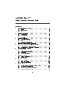
In the smooth case of (13), ��(x) = tanh(x � �) as depicted in Figure 3.
φ+ x x-
o
x+
φ-
Figure 3. The graphs of �� = tanh(x � �) with � > � � 0:957. 16 0
Edalat
For � > � where � � 0:957 is the root of the equation � = tanh 2�, the IFS is hyperbolic (since �0�(x) < 1 for all x 2 I ) and satis es � I \ �?I = ;. Therefore, for � > � , the support of the invariant measure is a Cantor set. For 0 < � < � , the IFS is not hyperbolic (since each �0� takes value 1 when �� vanishes), but it can be shown to satisfy the condition of Proposition 2.4; therefore, a unique invariant measure exists; furthermore, � I [ �?I = I , which implies that the support of the invariant measure is the whole interval. 0
0
+
0
0
+
Note that in all cases the invariant measure �� is given constructively by the unique xed point of the transition operator
T : P UI ! P UI � 7! � � �?? + � � �? : 1
1
1 2
1 2
1
1 +
In other words, �� = Fn� T n�I where, for n � 1, 0
T n�I = 21n
X i1 ;i2 ;:::;in =�
�� 1 � 2 :::� I : i
i
in
Using Elton's Theorem [8], we can now prove the following.
Theorem 5.1 The limiting distribution of the couplings of the marginalist and smooth models are given by the invariant measures of the corresponding IFSs with probabilities, the unique xed points of the transition operators on the domain P1 UI .
As an interesting application, one can use the above result to investigate the local behaviour of the limiting distributions, which is of basic theoretical as well as practical interest [2]. In fact, for any open subset a � I , we have
��(a) = supn� (T n�I )(2a) = supn� 0
0
X �i1 �i2 :::�in
1: n I �a 2
In this paper, however, we will use Equations (6) and (7) to compute the expected value of any physical quantity with respect to the distribution of the couplings. An important quantity is the decay rate of each stored pattern as new patterns are learned; this is used to compute the storage capacity of the net [2] and is de ned as follows. If patterns Xm , m = 1; : : : ; M , have been learned and encoded in the couplings Jij = JijM (i; j = 1; : : : ; N ) of a net, then the embedding strength [9] of pattern Xm is given by (
N X 1 Jij Xim Xjm: em = N i;j =1
17
)
Edalat
In forgetful nets the embedding strength of a pattern depends on its storage ancestry. That is, if n = M ? m, then em = eM ?n = e(n). The decay rate of e(n) with n is exponentially fast and is given by, e(n) � exp( n) as n ! 1 [2], where is the average Lyapunov exponent of the stochastic mapping (14), and is given by, Z
= 21 (ln �0 (x) + ln �0?(x)) d��(x): +
For the marginalist model, one immediately nds that = ln �N [2]. For the smooth case,
Z
= ? ln cosh(x + �) cosh(x ? �) d��(x); I
which can be accurately computed by the generalised Riemann integral as compared with the approximation obtained in [2]. First note that the function g : [0; 1] ! R with
g(x) = ? ln cosh(x + �) cosh(x ? �) is an analytic function in I with
jg(x) ? g(y)j � cjx ? yj for c = maxx?�x�x+ jg0(x)j. For � > � , we know that the associated IFS is hyperbolic, and therefore Equation (7), with k = 1 and s = 1=2, gives us a formula to compute the integral up to any threshold � > 0. 0
For 0 < � � � , when the associated IFS is not hyperbolic, we have an algorithm to compute the integral up to � > 0 accuracy, although we have not yet analysed its complexity. We will describe the algorithm and show its soundF � ness. Since � = n� T n�I 2 S I , by Proposition 2.2, with � = �=2 and = �=2c, there exists n � 0 such that 0
1
0
k < �=2 2n
(15)
where k is the number of lists hi ; i ; : : : ; ini (where i ; : : : ; in = �) of length n such that the diameter of the set �i1 �i2 : : : �i I is at least �=2c. 1
2
1
n
The generalised Riemann sum X g(�i1 �i2 : : : �i 0) S (g; T n�I ) = 21n i1 ;:::;i � 18 n
n=
Edalat
and the integral are both sandwiched between the corresponding lower and upper sums S ` and S u and we have
Su ? S` = 1 X (sup g(� : : : � I ) ? inf g(� : : : � I )) = i1 i i1 i 2n i1 ;:::;i � 1 X(sup g(� : : : � I ) ? inf g(� : : : � I ))+ i1 i i1 i 2n 1 X(sup g(� : : : � I ) ? inf g(� : : : � I )) i1 i i1 i 2n n
n
n=
n
n
n
n
1
2
where the rst summation is over those subsets whose diameters are less than �=2c and the second summation is over the rest of the subsets. By Equation (15), the rst term is < �=2, since 0 < g(x) � 1 for all x 2 R. By the Lipschitz condition, the second term is also < �=2, since the sum of the coe�cients 1=2n is at most 1. Hence, Z jS (g; T n�I ) ? g d��j < �: The algorithm, therefore, nds the least n � 0 such that the nth level of the IFS tree, equivalently T n�I , satis es Equation (15). Note that since �? and � are both monotone, the diameter of �i1 : : : �i I is simply +
n
�i1 : : : �i (x ) ? �i1 : : : �i (x? ): n
+
n
The algorithm then computes S (g; T n�I ).
Acknowledgement I would like to thank U. Behn for inviting me to the Physics Department at Leipzig University in the Summer of 1994 and for a number of informative discussions on forgetful neural nets.
References [1] M. F. Barnsley. Fractals Everywhere. Academic Press, second edition, 1993. [2] U. Behn, J. L. van Hemmen, R. Kuhn, A. Lange, and V. A. Zagrebnov. Multifractality in forgetful memories. Physica D, 68:401{415, 1993.
19
Edalat
[3] A. Edalat. Dynamical systems, measures and fractals via domain theory (Extended abstract). In G. L. Burn, S. J. Gay, and M. D. Ryan, editors, Theory and Formal Methods 1993. Springer-Verlag, 1993. Full paper to appear in Information and Computation. [4] A. Edalat. Domain of computation of a random eld in statistical physics. In Hankin et al, editor, Proceedings of the Second Imperial College, Department of Computing, Theory and Formal Methods Workshop. 1994. [5] A. Edalat. Domain theory and integration (Extended abstract). In Logic in Computer Science. IEEE Computer Society Press, 1994. Ninth Annual IEEE Symposium, July 3-7, 1994, Paris, France. Full paper to appear in Theoretical Computer Science. [6] A. Edalat. Power domains and iterated function systems. Technical Report Doc 94/13, Department of Computing, Imperial College, 1994. Submitted to Information and Computation. [7] A. Edalat. Domain theory in stochastic processes. In Proceedings of Logic in Computer Science, Tenth Annual IEEE Symposium, 26-19 June, 1995, San Diego. IEEE Computer Society Press, 1995. To appear. [8] J. Elton. An ergodic theorem for iterated maps. Journal of Ergodic Theory and Dynamical Systems, 7:481{487, 1987. [9] J. L. van Hemmen, G. Keller, A. Huber, and R. Kuhn. Nonlinear neural networks. Journal of Statistical Physics, 50(1/2):231{293, 1988. [10] J. L. van Hemmen, G. Keller, and R. Kuhn. Forgetful memories. Europhysics Letters, 5(7):663{668, 1988. [11] D. Hepting, P. Prusinkiewicz, and D. Saupe. Rendering methods for iterated function systems. In Proceedings IFIP Fractals 90. 1991. [12] J. J. Hop eld. In Proceedings of the National Academy of Science, USA, volume 79, page 2554. 1982. [13] J. J. Hop eld. Neurons with graded response have collective computational properties like those of two-state neurons. In Proceedings of the National Academy of Science, USA, volume 81, pages 3088{3092. 1984. [14] C. Jones and G. Plotkin. A Probabilistic Powerdomain of Evaluations. In Logic in Computer Science, pages 186{195. IEEE Computer Society Press, 1989. [15] S. Karlin. Some random walks arising in learning models. Paci c Journal of Mathematics, 3:725{756, 1953. [16] S. Lakshmivarahan. Learning algorithms theory and applications. Springer, 1981. [17] M. M�ezard, J. P. Nadal, and G. Toulouse. Solvable models of working memories. J. Physique, 47:1457{1462, 1986. [18] J. P. Nadal, G. Toulouse, J. P. Changeux, and S. Dehaene. Networks of formal neurons and memory palimpsests. Europhysics letters, 1(10):535{542, 1986.
20
Edalat
[19] M. F. Norman. Markov processes and learning models. Academic Press, 1972. [20] G. D. Plotkin. A powerdomain for countable non-determinism. In M. Nielsen and E. M. Schmidt, editors, Automata, Languages and programming, pages 412{ 428, Berlin, 1982. EATCS, Springer-Verlag. Lecture Notes in Computer Science Vol. 140. [21] N. Saheb-Djahromi. Cpo's of measures for non-determinism. Theoretical Computer Science, 12(1):19{37, 1980. [22] A. N. Shiryayev. Probability. Graduate texts in mathematics. Springer, 1984.
21