DRAFT – COMMENTS WELCOME WHAT CAUSED CHANGES IN HOUSEHOLD INCOME AND POVERTY IN RURAL SICHUAN IN THE EARLY 1990s? Neil McCulloch * Institute of Development Studies University of Sussex Brighton East Sussex, BN1 9RE UK Tel: 01273 877223 Fax: 01273 621202 Email:
[email protected] and Cao Yiying Chinese Centre for Agricultural Research Beijing China
Abstract The recent entry of China into the WTO has led to a heated debate about the impact of liberalisation upon the poor in China. Aggregate studies of growth and poverty are generally unable to identify the causal pathways through which policies impact upon households, whilst modeling approaches only provide plausible simulations of what may occur. This paper attempts to disentangle the empirical causes of changes in income and poverty transitions in Sichuan during in the early 1990s, a period of major reform. We find that poverty is highly dynamic with income and poverty changes driven by changes in income from farming and animal husbandry. We also find evidence that health, rainfall and grain market shocks have a strong impact on incomes whilst grain quota prices play a small but statistically significant role in social protection. Keywords: East Asia, China, chronic poverty, vulnerability, poverty dynamics JEL Codes: *
This paper was prepared as part of the DFID funded Globalisation and Poverty Research Program. The authors are grateful to DFID for financial assistance. In addition we are grateful to the International Development Research Centre for funding a visiting fellowship from the Chinese Centre for Agricultural Policy (CCAP) to ensure technical capacity building during the course of the project. Thanks are due to Julie Litchfield and L. Alan Winters who set up the project, the Household Survey Division of the Rural Survey Organization in the National Bureau of Statistics for supplying the data and to Zhang Shuying and Yan Fang for their invaluable assistance. Zhang Linxiu and Huang Jikun at the Center for Chinese Agricultural Policy provided information about anti-poverty policy in Sichuan. All errors remain the responsibility of the authors.
1
DRAFT – COMMENTS WELCOME 1. Introduction China is often hailed as one of the most successful examples of poverty reduction in history. The economic reforms initiated in 1978 led to a dramatic increase in the rate of economic growth. The average annual rate of growth of GDP was 10.2 per cent during the 1980s leading to a rapid decline in the proportion of the population below the official poverty line (Khan, 1998). Although estimates vary, all sources show a huge decline in poverty between the late 1970s and the mid 1980s - for example, a World Bank study estimated that the proportion of the rural population in poverty declined from 33 per cent in 1978 to 11 per cent in 1984 (World Bank, 1992). The decline in poverty slowed considerably in the second half of the 1980s and the early 1990s and even reversed in some locations, but strong growth and poverty reduction was re-established by the mid1990s. However, studies of income growth and poverty reduction in the aggregate are rarely able to disentangle the myriad causes for movements into and out of poverty or to link such causes to variables under the direct influence of policy. Yet an understanding of the relative importance in determining incomes of demographic shocks, changes in endowments, economic shocks, illness, policy shocks and initial conditions, can help in the design of appropriate policies to reduce poverty. Furthermore, there is a hotly contested debate about the impact of particular policies of liberalisation upon the poor. At the national level several studies have attempted to predict the impact of different facets of China’s recent entry into the WTO on growth and poverty reduction (Huang and Rozelle, 2002, Hussain, 2002, Ianchovichina and Martin, 2002, Sicular and Zhao, 2002). However, it is also important to know empirically what the actual effects of previous policy interventions have been and this entails disentangling these effects from those of the many other things going on at the same time. For example there was a dramatic shift in grain market policy during the early 1990s – it is important to know to what extent this policy change gave rise to the observed movements into and out of poverty. This paper looks at the causes of changes in income and poverty in rural Sichuan. Sichuan’s growth and poverty reduction performance appears to have mirrored that of China as a whole with growth rates of over 10% each year in the early 1990s. McCulloch and Calandrino (2003) show that poverty levels in the province stagnated between 1991 and 1993, but then fell rapidly in 1994 and 1995. They also draw on a five year panel of households to provide evidence for considerable economic mobility with many households experiencing a high level of variability in their consumption over time causing many to enter or exit poverty. Given China’s impressive performance in reducing poverty, and the fact that Sichuan is, in many respects, a microcosm of China, it is of particular interest to understand the reasons for movements in income and poverty in Sichuan. The paper is arranged as follows: the next section briefly describes the five year panel data set available for rural Sichuan; the subsequent section details our approach to the analysis of income and poverty dynamics – in particular for both income and poverty we attempt to first describe the changes which took place, decompose them into their
2
DRAFT – COMMENTS WELCOME constituent elements, and then explain the proximate causes for the observed changes. We conclude with the implications of our findings for policies which are likely to impact upon poverty.
2. Data The data which we use are from a five year panel of 3311 households in rural Sichuan from 1991 to 1995. This data was collected by the Household Survey Division of the Rural Survey Organization in the State (now National) Bureau of Statistics. The administration of the Rural Household Survey (RHS) has been described in detail elsewhere (Chen and Ravallion, 1996). However, it is worth highlighting some of the key features of the RHS since they impact strongly upon the quality and reliability of the data. Firstly the RHS is administered directly by the NBS through its provincial and local survey network. This ensures that the data collected are free from interference by local governments. Secondly, rather than employing a single interview approach, each selected household maintains a daily diary over the entire year as well as two transaction books – one for cash transactions and one for goods. An assistant interviewer is supposed to visit each household every two weeks to check the books, assist the household in filling them in and transfer the information to the county level. The assistant interviewer is usually a cadre and is therefore familiar with the local area and has a secondary school qualification. A member of the county level team visits each household once a month. The unusual rigor applied to the collection, checking and processing of the RHS data means that the RHS is less likely to suffer from a variety of non-sampling errors common to household surveys in many other countries. The survey questionnaire collects a large amount of socio-economic information about the community, the local area, the household and its members and their assets and economic activities.1 In particular, the data set contains detailed information on both household income and consumption. Gross income comprises both cash income and goods in kind, and is broken into wage income, family business income, transfer income and asset income. Net income is gross income minus family business expenditures, depreciation, tax, payments to the collective and the survey subsidy. Furthermore, family business income can be broken down by sector, by far the largest of which are farming (of which grain sales are the most important) and animal husbandry. Most quantitative studies of poverty in the developing world use consumption data because this is generally deemed to be more reliable than income data and because consumption is an outcome variable which takes into account the ability of the household to smooth income over time. However, our particular interest here is to understand the causes of movements in and out of poverty. In many cases such movements may result from changes in income from particular sources. We therefore use income rather than consumption as our welfare indicator since it allows us to examine more closely how policy and other factor affect the level of resources available to the household.2 1 2
See (McCulloch and Calandrino, 2002) for details. See (McCulloch and Calandrino, 2003) for an analysis using the consumption data.
3
DRAFT – COMMENTS WELCOME
Our estimates of household income were divided by the number of adult equivalents in the households using the World Health Organization adult equivalence scale presented in Appendix 1. This scale is derived from detailed studies of the nutritional requirements of males and females of different ages in developing countries (West, et al., 1988).3 The Consumer Price Index used to deflate nominal variables is taken from the published data in the China Statistical Yearbook for rural Sichuan. It is based on a basket of 382 commodities and services and compounds the year-on-year rates using 1991 as the base year.4 Published data for 1991 to 1993 used an (unknown) mix of market and official prices, rather than market prices to value certain goods which may give an underestimate of the rate of increase of consumer prices (and therefore an overestimate of the improvement in real incomes and consumption). Unfortunately, we have no means of correcting this since we do not have any information on the market prices of the goods included in the basket.5 Published price indices for 1994 and 1995 appear to use free market prices and so we have used these values. Measurement Error Income measures from household surveys are notoriously susceptible to measurement error. Although from an econometric point of view, additional noise in the dependent variable will not affect the consistency of estimates6, this noise will be amplified when examining changes in income which is our particular concern here. Therefore we have adjusted our income measure using the method described in (McCulloch and Baulch, 2000). This method exploits the fact that consumption and income tend to be well correlated and therefore can be used as instruments for each other in econometric models.7 It constructs a simple model in which the ‘true’ real adult equivalent income of household i in year t (i.e., uncorrupted by measurement error), y*it, is a function only of its value in the previous year – that is:
y*it = ρy*i,t −1 + ε it
(1)
where εit is an error term which is assumed to be uncorrelated with past income. If income is measured with error, then estimating this model using measured income will
3
No adjustment was made for economies of scale within the households. This is because estimates in the literature of the extent of household economies of scale vary considerably (Lanjouw and Ravallion, 1995) and the profession does not currently have an acceptable theory for how to handle differing needs and economies of scale. See (Deaton, 1997) for an exposition of the theory and the debate over the identification of equivalence scales; (Deaton and Muellbauer, 1980, Deaton and Muellbauer, 1986) provide a detailed description of the theory. A recent paper by (White and Masset, 2002) claims to provide a practical solution to the identification problem. 4 Note that since the CPI is a year-on-year Paasche index, compounding in this way yields a mixed index rather than a true Paasche index for the whole period. 5 It is not advisable to use our dataset to correct for these since our panel data contains information on only 17 commodities. 6 As long as the measurement error is uncorrelated with the regressors. 7 For example, (Altonji and Siow, 1987) use this technique to obtain unbiased estimates of the response of consumption to changes in income.
4
DRAFT – COMMENTS WELCOME σ2 yield an estimate of ρ that is biased towards zero by 1 − m2 where σ2m is the variance σ y 2 of the measurement error and σ y is the variance of observed income. However, an unbiased estimate of ρ can be obtained by estimating the model using consumption in ρ − ρ OLS then provides an estimate year t-1 as an instrument for measured income; IV ρ IV
of the ‘noise-to-signal’ ratio σ2m/σ2y. We estimate this ratio using both consumption and lagged income as instruments in order to obtain an indication of the magnitude of measurement error. An adjusted income variable is then constructed which shares the same estimated mean as the true income variable but has the estimated variance of the true income variable rather than that of the observed income. The adjusted income variable is: σ y* (2) a it = y i + (y it − y i ) σ y where y i is the inter-temporal mean of the observed income of household i and σ y* is the standard deviation of “true” income. Under the assumption above that the measurement error has a zero mean, the expected value of y i is equal to the expected value of true income; deviations from this expected value are scaled by the estimated ratio of the standard deviation of true income to the standard deviation of observed income. Poverty Line
The poverty line is composed of food and non-food components. The food poverty line is based on the cost of the nutritional requirements of individuals – set at 2100 kilocalories per day – with weights determined by the composition of food consumption of families around the poverty line. In 1994 the food poverty line was Yuan 452. The non-food component was estimated using the food share regression methodology presented in (Ravallion and Bidani, 1994) estimated using data from 5500 families in Sichuan in 1994. Low and high poverty lines were calculated: the low poverty line has a non-food component equal to the expenditure on non-food items of those households whose total expenditure is equal to the food poverty line – this can be regarded as a lower limit of essential non-food expenditure, since these households are choosing to spend on these items at the expense of meeting their nutritional needs; the high poverty line is based on the non-food expenditure of those whose food expenditure is equal to the food poverty line – that is, the typical non-food expenditure of those who just meet the nutritional standard. A further adjustment was made to take account of the fact that food for own-consumption was valued at market prices despite being of lower quality, and to translate per capita poverty lines into per adult equivalent poverty lines. This yielded per adult equivalent lower and upper poverty lines for 1991 of 409 and 457 Yuan
5
DRAFT – COMMENTS WELCOME respectively. These are similar to the poverty lines suggested by (Tong and Mingang, 1995).8
3. Analysing Income and Poverty Dynamics There are a large number of different ways in which income and poverty dynamics may be analysed (see (Bradbury, et al., 2001, Walker and Ashworth, 1994) for reviews of methods). We focus on three approaches to the analysis of income dynamics and the corresponding methods for the analysis of poverty dynamics. These three approaches can be broadly characterised as description, decomposition and explanation and are illustrated in Table 1. Table 1: Techniques for description, decomposition and explanation of income and poverty dynamics
Description Decomposition
Explanation
Income Quantile transition matrices Mobility indices Explaining income changes in terms of changes in the number of adult equivalents and changes in income from different sources Dynamic panel regressions of income against household and community characteristics
Poverty Poverty transition matrices Explaining poverty changes in terms of changes in the number of adult equivalents and changes in income from different sources Switching regressions of income against household and community characteristics
Techniques for describing the extent of income dynamics typically focus on the production of quantile transition matrices (usually by quintile or decile) and the calculation of associated aggregate mobility measures. Alternatively a different class of mobility measures may be constructed from estimates of aggregate inequality. As poverty is a discrete rather than a continuous state, descriptions of poverty dynamics tend to use poverty transition matrices centered around a poverty line rather than an arbitrary set of quantiles. Decomposition methods for income changes simply exploit the fact that real adult equivalent incomes comprise two components – real household income and the number of adult equivalents – and the relative influence of these components can therefore be calculated. The real household income component can be similarly decomposed into different income sources. Decomposition methods for poverty changes use the same methods but focus on the changes which have actually given rise to poverty transitions. Finally, “explanatory” techniques attempt to address how household and community characteristics and their changes (e.g. educational level of the members, assets, prices of 8
McCulloch & Calandrino (2002) provide full details of the construction of the poverty lines.
6
DRAFT – COMMENTS WELCOME key commodities) may have given rise to the observed changes in income and poverty using panel data regression methods.
4. Describing Income and Poverty Dynamics The starting point in understanding movements in income and poverty is to appreciate the extent of such movements. We therefore calculated quintile transition matrices for each consecutive pair of years. Table 2 shows the quintile transition matrix using adjusted income in 1991 and 1992.9 Table 2: Relative Quintile Transition Matrices 1991-92 Percentage of households from 1991 quintile in 1992 quintile 1992 quintile 1 2 3 4 5 53.6 26.4 12.6 5.7 1.7 25.4 31.5 23.9 14.0 5.3 13.0 22.0 30.7 24.3 9.9 5.7 15.8 21.1 31.3 26.1 2.2 4.4 11.8 24.7 57.0
real net income 1991 quintile 1 2 3 4 5
Table 2 shows a very degree of income mobility, even after income has been adjusted for measurement error. Almost half of the households in the bottom quintile in 1991 move to a different quintile in 1992, whilst a quarter of those in the second quintile fall into the bottom quintile (the bottom quintile is Yuan 472 in 1991 – the upper poverty line is Yuan 457, the lower poverty line is Yuan 409). Examining the transition matrices between other years in the panel shows that mobility increases over the years, with only around 49% of households remaining in the bottom quintile between 1992 and 1993 and only 48% of households remaining in the bottom quintile between between 1993 and 1994 and between 1994 and 1995. To assess the extent to which overall mobility has changed over the period we calculated values for a set of mobility measures commonly used in the literature for each consecutive pair of years in our panel – the results are shown in Table 3 (see (Fields, 2002) for a review of mobility measures). Table 3: Mobility Measures for relative income quintiles Year 91-92 92-93 93-94 94-95 9
Trace Mobility 0.59 0.61 0.61 0.60
More Than One Mobility 0.20 0.23 0.23 0.20
Distance Mobility 0.27 0.28 0.28 0.27
All tables show results using adjusted income unless otherwise noted.
7
DRAFT – COMMENTS WELCOME
Table 3 confirms the high level of mobility suggested by looking at individual quintiles in the transition matrices. The Trace Mobility measure shows that around 60% of households change quintile between each consecutive pair of years10, with a fifth or more moving More Than One quintile. The Distance Mobility measure calculates the ratio of actual quintile movements to the maximum possible movement, with households on average travelling more than a quarter of the maximum possible distance. Tables 2 and 3 show relative mobility between quintiles of different years. However, income were increasing on average over the period. It is therefore useful also to examine absolute mobility. Table 4 shows the absolute quintile transition matrix between 1991 and 1995. This shows that only 36% of those who were in the bottom quintile in 1991 were in the same absolute income quintile (i.e. fixed at the 1991 level) in 1995. By contrast 62% of those who were in the top income quintile in 1991 were in the same income bracket at the end of the panel. Table 4: Absolute quintile transition matrix 1991-95 real net income 1991 quintile 1 2 3 4 5 Total
1
2 35.8 19.8 13.5 6.8 3.6 15.9
25.7 20.0 16.9 11.6 4.4 15.7
1995 quintile 3 18.0 21.2 22.3 16.4 11.8 18.0
4
5 12.7 21.1 25.9 28.4 18.3 21.3
7.8 17.8 21.4 36.7 62.0 29.1
As before, aggregate mobility measures can be calculated for absolute income quintiles. Table 5 shows the aggregate mobility measures when quintiles are fixed at their 1991 values. Table 5: Mobility Measures for absolute income quintiles Year
Trace Mobility
91-92 92-93 93-94 94-95
0.59 0.62 0.63 0.60
More Than One Mobility 0.21 0.24 0.26 0.22
Distance Mobility 0.27 0.29 0.31 0.28
Upward Mobility 0.23 0.19 0.33 0.25
Downward Mobility -0.20 -0.28 -0.16 -0.20
Table 5 again shows a high level of income mobility. However, using fixed “quintile” values allows us to disaggregate the distance mobility measure into upward and downward distance measures. This shows that there was a large general upward movement between 1993 and 1994 and again between 1994 and 1995. For example, 10
This is a higher figure than for the bottom quintile because the central three quintiles are more mobile by construction than the bottom and top quintiles since the former cannot move down and the latter cannot move up.
8
DRAFT – COMMENTS WELCOME households who moved up absolute income quintiles between 1993 and 1994 moved by one third of the maximum possible distance which they could have moved, whereas households who moved down during the same period moved by only 16% of the possible downward movement. It is also interesting to note that there was a large downward movement between 1992 and 1993.11 The existence of a high level of income mobility overall does not necessarily mean that there is a large amount of movement in and out of poverty. To determine the extent to which poverty is dynamic we calculated poverty transition matrices. These show that only 28% of households who were poor in 1991 were poor in 1995. Furthermore, to show the extent of income movement among the poor and non-poor separately, the intertemporal mean income (across the five years of the panel) was calculated for each household. Table 6 shows the number of households whose intertemporal mean income is below or above the lower poverty line against their income poverty status in 1991. Table 6: Poverty status in 1991 by Intertemporal poverty status Intertemporal mean income Below poverty Above poverty Total Poor 123 226 row% 35.24 64.76 col% 70.69 7.41 Non-poor 51 2824 row% 1.77 98.23 col% 29.31 92.59 Total 174 3050 row% 5.4 94.6 col% 100 100
349 100 10.83 2875 100 89.17 3224 100 100
Table 6 shows that slightly more than one third of those who were income poor in 1991 had an intertemporal mean income below the poverty line across the five years. Thus households who were poor at the beginning of the panel have experienced a large amount of movement. Moreover, 29% of those households whose intertemporal income is below the poverty line were not poor in 1991. Such descriptive exercises suggest that there is a great deal of income mobility both amongst the general population and amongst the poor. But what is driving this mobility? The next section decomposes the elements of real per adult equivalent income to shed light on the balance between changes in the number of adult equivalents and the changes in different income sources giving rise to the observed high level of income mobility. The following section seeks to understand the factors responsible for poverty transitions.
5. Decomposing the changes in adult equivalent income
11
These results are also reflected in the cumulative distributions of income for each of the five years – see McCulloch and Calandrino (?? working paper) for details.
9
DRAFT – COMMENTS WELCOME Per adult equivalent income, of course, consists of the ratio of household income and the number of adult equivalents in the household. Changes in per adult equivalent income can therefore result from changes in household income or changes in the demographic composition of the household or both. However, from a policy perspective, it is useful to know whether such changes arise predominantly from changes in household income, or from changes in the household structure. The change in per adult equivalent income can be decomposed into three components: the percentage change in household income times the base year per adult equivalent income; negative the percentage change in the number of adult equivalents times the base year per adult equivalent income; and a residual term. More precisely:
Y ∆Y Yt −1 − ∆A Yt −1 − ∆A ∆Y Yt −1 + + ∆ = A Yt −1 At −1 At −1 At −1 At −1 Yt −1 At −1
(3)
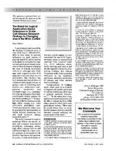
where Y is household income and A is the number of adult equivalents; time subscripts indicate the year. The graphs in Figure 1 plot the income component of equation 1 (the first term on the right hand side) by the adult equivalent component, both normalised by the overall change in per adult equivalent income, for each household and each consecutive pair of years. If the change is entirely due to changes in household income, the household will be plotted at point (0,1) – similarly if the change is entirely due to changes in the number of adult equivalents then the household will be plotted at (1,0). The extent to which points are concentrated at one end of the line running between these two points indicates the relative importance of income changes and changes in the number of adult equivalents, whilst the extent to which points are “off” the line indicates situations in which both household income and the number of adult equivalents have changed. The left hand graph in Figure 1 plots the normalised income and adult equivalent components between –5 and +5. This shows that in many instances (28%) the income component is greater than one. This implies that the percentage change in household income is in the same direction as the percentage change in per adult equivalent income but with a larger absolute magnitude. For example if household income increases by a larger percentage than the increase in per adult equivalent income, then it must be the case that there was also an increase in the number of adult equivalents (implying a negative adult equivalent term). When the adult equivalent term is larger than one (which is true in 7% of the cases) this implies that the percentage change in income has been in the opposite direction from the change in per adult equivalent income implying that there has been a compensating movement in the number of adult equivalents. For example, if per adult equivalent income rises, but household income falls, then the number of adult equivalents must also have fallen (causing a positive adult equivalent term). The points lying between coordinates (0,1) and (1,0) represent the 30% of cases where household income changes in the same direction as per adult equivalent income but by a smaller absolute magnitude – for example if household income rises and the number of adult equivalents also falls (or if household income falls and the number of
10
DRAFT – COMMENTS WELCOME adult equivalents also rises). The remaining 35% of all cases are situations in which only household income changes. The second graph plots points between (0,1) and (1,0). The clustering of the points in the top left hand corner of this graph suggests that, for situations where household income changes in the same direction as per adult equivalent income but by a smaller absolute magnitude, the bulk of the change in per adult equivalent income results from changes in household income rather than changes in the number of adult equivalents. This is true in general, with the absolute value of the income component being larger than that of the adult equivalent component in 87% of cases. The importance of income changes in determining most changes in per adult equivalent income suggests that it would be helpful to examine further the different components of income to understand which income sources are typically giving rise to changes in household income. Table 7 shows the sources of household income broken down by quintiles of mean per adult equivalent income across the five years of the panel. The wage share increases with household income, from 12 per cent for the bottom quintile to 18 per cent for the top quintiles. Conversely the share of profits from family business in total income decreases from 83 per cent to 75 per cent between the bottom and top quintiles. The remaining income categories represent only a small proportion of total income. The share of net remittances lies between 2 and 2.5% for all quintiles, while transfers are rather regressive accounting for 1.4 per cent of the income of households in the poorest quintile but 3.6 per cent of the income of the richest households.
11
DRAFT – COMMENTS WELCOME
Figure 1: Relative importance of Income and Adult equivalent changes
1
inocme component
inocme component
5
0
-5
.5
0 -5
0 adult equivalent component
5
0
.5 adult equivalent component
1
12
DRAFT – COMMENTS WELCOME
Table 7: Income Shares by Inter-temporal Mean Income Quintiles Intertemporal % income share of: mean income profits wages net transfers asset quintiles remittances income 1 (poorest) 83.5 11.9 2.2 1.4 0.9 2 80.3 14.2 2.5 2.1 1.0 3 79.5 15.0 2.2 2.2 1.1 4 77.7 16.2 2.1 2.8 1.2 5 (richest) 74.8 18.2 2.0 3.6 1.4 Note: this table uses unadjusted income since it is not reasonable to assume that all income sources have the same error variance. However, since the table present shares of income the results are similar to those for adjusted income.
Although Table 7 shows that profits are the most important source of income, this does not necessarily mean that changes in profit income are the principle cause of changes in household income since some sources of income may be more “constant” than others. In the extreme case one might have a source of income with a high share of income but which was completely constant over time; if this was the case then it would contribute nothing to the changes in income even if it contributed a large share to the level of income. To explore this further we regressed each component of income separately on household income12; the coefficients from such descriptive regressions provide a robust approximation to the income shares of each component.13 We then regressed the change in each income source against the change in household income; the coefficients from this regression indicate the average share of the change in income arising from each source. Note that in the example above of a constant income source, the former regression would correctly show the high share of income coming from the constant source, whilst the latter regression will have a coefficient of zero, indicating that none of the income changes resulted from changes in the (constant) component. Table 8 shows both sets of coefficients, along with the average inter-temporal coefficient of variation for each income source. Table 8: Level and change coefficients for income sources Share of income coefficient Profits Wages Net remittances Transfers Assets
0.779 0.156 0.024 0.028 0.013
Share of change of income coefficient 0.780 0.136 0.023 0.018 0.010
Average Intertemporal coefficient of variation 0.35 1.13 1.32 1.55 1.74
12
The regressions are constrained to pass through the origin to ensure adding up. An alternative to this approach would be to average the income shares. However, this will not necessarily give the same result and is more sensitive to the presence of extreme outliers than the regression approach. 13
13
DRAFT – COMMENTS WELCOME Note: this table uses unadjusted income for the reasons described above. Results for shares from adjusted income are the same; results for profit share of changes is somewhat lower.
Table 8 shows that, although in principle the share of changes in income could be different from the share of income, in practice this difference is small. Just as 78% of household income comes from profits, so it is true that on average 78% of changes in household income result from changes in profit income. The shares of changes of income are similar to the shares of income for all income sources except transfers, which contribute somewhat less to changes in household income than their (small) share of household income. The third column of Table 8 shows that profit income is substantially less variable across time than other income sources, with a standard deviation across time only around a third of the inter-temporal mean value of profit income. By contrast, all other sources of income are highly variable with assets income the most variable with a standard deviation of 174% of its mean value. Given the importance of changes in profit income for changes in overall household income, it is useful to further disaggregate this term. Profit income consists of the gross income from farming, animal husbandry, and other family business income14 minus costs, depreciation of assets and tax. Table 9 shows the results from regressing the real income from each component of profits on profit income, as well as regressing the change in each component against the change in profit income. Table 9: Level and change coefficients for profit income Profits
Share of profit coefficient
Share of change of profit coefficient 0.29 0.10 0.36 0.36
Farming 0.74 - of which grain sales 0.40 Animal Husbandry 0.55 Other family business 0.30 income Costs 0.52 0.02 Depreciation 0.04 0.00 Tax 0.03 0.00 Note: revenues and expenditures are expressed as percentages of profit. Again unadjusted income is used. The results are very similar with adjusted income.
As expected we see that the bulk of profits comes from farming income – indeed grain sales on their own typically constitute 40% of profit income. Animal husbandry is also an extremely important part of profit income, with revenue from this source equal to more than 50% of profit income. However, unlike above, the typical change in each of these sources of revenue and expenditure as a share of the change in profit is not equal to their share of profit income. For example, although revenue from farming constitutes almost three-quarters of profit 14
From forestry, fishery, handicraft, collecting/hunting, industry, construction, transportation, commerce, catering, services and other income.
14
DRAFT – COMMENTS WELCOME income, changes in farming revenue only make up 29% of changes in profit income. The main reason for this is that reported changes in costs only make up 2% of change in profits, even though expenditures on family businesses amount to more than 50% of profit income. This suggests that households have only reported fixed costs, thus leading to an underestimate of the role of changes in variable costs in changes in profits. However, even if this is the case the ranking of the share of changes in revenue sources in changes in profit is different from their shares in the level of profit income. This does suggest that other family business income is somewhat more volatile than animal husbandry, which in turn is more variable than income from farming and particular income from grain sales. Since income from grain sales is to some extent determined by government policy, this suggests that grain policy may have helped to stabilise income from this particular source.
6. Decomposing movements in and out of poverty The above section focussed on decomposing movements in the continuous income variable. However, we are particularly concerned with changes in income which give rise to movements into or out of absolute poverty. We therefore decompose movements in and out of poverty by assigning the principle cause of the change.15 Table 10a shows the principle causes of movements into poverty for each pair of years; table 10b shows the principle causes for movements out of poverty (using the lower poverty line). Interestingly for both moving in and out of poverty, changes in household income are generally much more important than changes in the number of adult equivalents in the household, with over 90% of entries into and exits from poverty resulting from income rather than demographic changes. Furthermore, it can be shown that the relative importance of household income changes is even greater for poverty transitions than for movements in per adult equivalent income generally, since demographic changes contribute more to changes in per adult equivalent income than household income changes for 14% of households who do not change poverty status, whereas this is true for only 5% of those who fall into poverty and 7.5% of those who exit poverty on average. Of course, this does not imply that major demographic events are not responsible for movements in and out of poverty – for example if the household head’s contribution to household income is larger than their share of the number of adult equivalents in the household (which will often be the case), then a household which falls into poverty because of the loss of this income through the death or illness of the household head will still be (correctly) classified as falling into poverty primarily because of a change in household income.
15
The largest cause is defined as the cause which has the largest share of the overall change.
15
DRAFT – COMMENTS WELCOME
Table 10a: Principle causes of movements into poverty Largest Cause of Falling into Poverty Change in adult equivalents Change in household income Change in employment income Change in remittances Change in transfer income Change in asset income Change in profits Change in farming income Change in livestock income Change in other business income Change in costs Change in tax or depreciation
1991-1992 4.8 95.2 3.5 0.0 0.4 0.0 91.2 56.4 24.2 7.0 3.5 0.0
% of households for whom this was the largest cause 1992-1993 1993-1994 3.7 5.6 96.3 94.4 5.4 3.3 0.5 1.4 0.0 0.5 0.0 0.0 90.4 89.3 59.3 39.7 21.0 34.1 5.2 10.3 4.0 3.7 1.0 1.4
1994-1995 5.2 94.8 4.1 0.5 0.0 0.5 89.6 40.4 35.8 8.8 2.6 2.1
% of households for whom this was the largest cause 1992-1993 1993-1994 12.9 6.7 87.1 93.3 8.6 4.8 3.8 0.5 0.5 0.0 0.0 0.2 74.2 87.7 38.3 57.1 22.5 19.8 9.6 4.1 2.9 6.3 1.0 0.5
1994-1995 8.1 91.9 3.3 1.1 0.4 0.0 87.1 48.9 25.7 7.0 4.8 0.7
Table 10b: Principle causes of movements out of poverty Largest Cause of moving out of Poverty Change in adult equivalents Change in household income Change in employment income Change in remittances Change in transfer income Change in asset income Change in profits Change in farming income Change in livestock income Change in other business income Change in costs Change in tax or depreciation
1991-1992 3.4 96.6 6.8 0.0 0.4 0.0 89.4 51.3 28.4 6.4 3.0 0.4
16
DRAFT – COMMENTS WELCOME Of the over 90% of households for whom a change in household income is the most important cause of the poverty transition, the overwhelming majority experience a larger change in profits than in any other source of income. Only 3-5% of the households in this panel fell into poverty because of a change in employment income and only 3-8.6% rose out of poverty for this reason. It is therefore rather important to understand what gave rise to these changes in profits. Decomposing this shows that changes in farming income and livestock income are the two most important reasons for changes in profits. However, the proportion of households for whom these are the most important causes fluctuates considerably from year to year: over half of the households falling into poverty at some point between 1991 and 1993 did so because of changes in farming income, whereas only 40% fell for this reason between 1993 and 1995. Conversely between a fifth and a quarter of households fell into poverty between 1991 and 1993 because of changes in livestock income, whereas over one third of households fell for this reason between 1993 and 1995. By contrast, the proportion of households exiting poverty primarily because of changes in farming income fell sharply from 51% between 1991-92 to 38% between 1992-93, probably reflecting a combination of grain policy and the drought of 1993. And, as the proportion of households falling into poverty because of changes in farming income fell between 1993 and 1995, so the proportion of households rising out of poverty for this reason between these years rose, again potentially reflecting changes in grain policy. Similarly as the proportion of households falling into poverty because of changes in livestock income rose between 1993-94, so the proportion of households moving out of poverty between these years for this reason fell (although the share was larger between 1994-95). The share of households falling into or rising out of poverty due to changes in other components of profits was generally much smaller, although over 10% of those who fell into poverty between 1993-94 did so because of changes in other (non-farming or livestock) business income). Tables 10a and 10b above indicate the largest single causes of movements in and out of poverty. However, there are usually multiple causes for entries or exits from poverty for any individual household. It is useful therefore to try and obtain some indication of the relative importance of different causes, rather than categorising households by the single largest cause. Table 11a and 11b show for each consecutive pair of years the percentage of households experiencing a corresponding change in each cause; for example Table 11a shows that 59.9% of the 227 households who fell into poverty between 1991 and 1992 experienced an increase in the number of adult equivalents in the households, while 95% of these households experienced a fall in profit income. The tables also show the median size of the change and the median percentage change. Finally the median share of each cause in the overall change is indicated.16 Tables 11a and 11b confirm the picture presented above that changes in profit income drive movements into (out of) poverty with typically over 90% of households falling into (rising out of) poverty experiencing some fall (rise) in profit income. 16
Medians are reported rather than means in order to try and indicate the typical value of each change and to provide results more robust to outliers.
17
DRAFT – COMMENTS WELCOME Table 11a: Relative importance of different causes of entering poverty (lower poverty line) Year
1991-92
1992-93
1993-94
1994-95
Causes
n = 227 Adult equivalent Profits Employment income Net remittances Transfers Asset income n = 405 Adult equivalent Profits Employment income Net remittances Transfers Asset income n = 214 Adult equivalent Profits Employment income Net remittances Transfers Asset income n = 193 Adult equivalent Profits Employment income Net remittances Transfers Asset income
Median percentage change
Median share in overall change*
0.1
1.5%
3.5%
94.7% 50.7%
-575.1 -0.5
-32.7% -3.8%
83.2% 0.1%
18.5% 44.5% 38.3%
0.0 0.0 0.0
0.0% -4.1% 0.0%
0.0% 0.0% 0.0%
47.9%
0.0
0.0%
0.0%
94.3% 52.3%
-659.7 -11.9
-38.6% -27.6%
82.4% 1.3%
22.0% 44.4% 31.4%
0.0 0.0 0.0
0.0% -32.3% 0.0%
0.0% 0.0% 0.0%
52.8%
0.0
0.6%
0.8%
91.1% 43.9%
-684.7 0.0
-39.9% 0.0%
83.6% 0.0%
28.0% 31.8% 4.7%
0.0 0.0 0.0
0.0% 0.0% 117.8%
0.0% 0.0% 0.0%
43.5%
0.0
0.0%
0.0%
93.3% 46.6%
-670.8 0.0
-41.0% 0.0%
81.1% 0.0%
25.9% 26.9% 33.2%
0.0 0.0 0.0
0.0% 0.0% 0.0%
0.0% 0.0% 0.0%
Percentage of households experiencing corresponding change when entering poverty
Median size of change
59.9%
(1991 Yuan)
* For the Adult equivalent cause, the median share in overall change indicates the median value of the adult equivalent component of the household income/adult equivalent decomposition described above of all those households which fell into poverty. The median share in overall change for the income terms indicates the change in the income component divided by the change in household income.
18
DRAFT – COMMENTS WELCOME Table 11b: Relative importance of different causes of exiting poverty (lower poverty line) Year
1991-92
1992-93
1993-94
1994-95
Causes
n = 236 Adult equivalent Profits Employment income Net remittances Transfers Asset income n = 209 Adult equivalent Profits Employment income Net remittances Transfers Asset income n = 415 Adult equivalent Profits Employment income Net remittances Transfers Asset income n = 273 Adult equivalent Profits Employment income Net remittances Transfers Asset income
Median percentage change
Median share in overall change*
0.0
0.0%
0.0%
92.4% 58.1%
506.4 23.7
38.9% 55.5%
78.6% 3.6%
21.6% 30.9% 19.5%
0.0 0.0 0.0
0.0% 0.0% 0.0%
0.0% 0.0% 0.0%
39.2%
0.0
0.0%
0.0%
83.3% 45.5%
449.4 0.0
39.8% 0.0%
79.7% 0.0%
25.8% 24.9% 4.3%
0.0 0.0 0.0
0.0% 0.0% 0.0%
0.0% 0.0% 0.0%
26.3%
0.0
0.0%
0.0%
91.3% 49.4%
628.1 0.0
58.5% 13.3%
76.8% 0.2%
26.5% 21.9% 45.5%
0.0 0.0 0.0
0.0% 0.0% 156.0%
0.0% 0.0% 0.0%
31.5%
0.0
0.0%
0.0%
93.4% 45.8%
688.8 0.0
59.4% 0.0%
82.2% 0.0%
25.6% 22.3% 32.2%
0.0 0.0 0.0
0.0% 0.0% 0.0%
0.0% 0.0% 0.0%
Percentage of households experiencing corresponding change when entering poverty
Median size of change
28.0%
(1991 Yuan)
* For the Adult equivalent cause, the median share in overall change indicates the median value of the adult equivalent component of the household income/adult equivalent decomposition described above of all those households which fell into poverty. The median share in overall change for the income terms indicates the change in the income component divided by the change in household income.
19
DRAFT – COMMENTS WELCOME However, changes in profit income are far from the only changes taking place. Around half of households falling into poverty experience an increase in the number of adult equivalents. A similar proportion of households falling into poverty experience a fall in employment income, around a fifth experience a fall in net remittances and typically over a third lose transfer and asset income. However, the size of these other changes is generally much smaller than changes in profit income. The median fall in profit income of those falling into poverty is between Yuan 575 and Yuan 685 – other income sources may be important in individual cases but because a similar number of households falling into poverty experience an increase in these sources as experience a decrease, the median change of those falling into poverty is close to zero. For example, the median change in employment income of those households falling into poverty between 1991 and 1992 is a mere Yuan 0.5, but for the 51% of these households who experienced a decline in employment income the median fall was Yuan 130. This was counteracted by the 49% of these households who experienced a median increase of Yuan 89. This is further illustrated by examining the median percentage changes for each source. Although profit income again typically shows the largest percentage change, other sources of income feature strongly in particular years. For example, both employment income and transfers fell by an average of close to a third between 1992 and 1993 for those households who fell into poverty, although the size of these changes was small. However, the small size of most movements in other sources of income and the balancing out of positive and negative movements mean that their overall contribution to the change in household income is minimal. Changes in profit income, by contrast, typically constitute over 80% of the change in household income. Table 11b shows a similar picture for movements out of poverty. The vast majority of households moving out of poverty experience an increase in profit income, but between 45-60% also experience increases in employment income, and between a fifth and around a quarter experience an increase in net remittances or transfers. The numbers experiencing an increase in asset income varies greatly across the years. Again the median size of movements in other income sources (and in the number of adult equivalents) is usually zero, whereas the median increase in profit income varies between Yuan 449 and Yuan 689. Profits typically increase by almost 40% each year between 1991 and 1993 and by almost 60% each year between 1993 and 1995. The median percentage increase in employment income is important between 1991-92 and non-trivial between 1993-94, but all other sources of income rise as much as they fall for households exiting poverty. Consequently changes in profit income constitute the only major contributor to the overall change in household income. The above decomposition of the movements into and out of poverty make it clear that changes in profit income and, in particular, farming and livestock income are the principle causes of both entry into and exit from poverty in rural Sichuan. Given the dependence of the rural poor in Sichuan on these sources of livelihood this is hardly surprising. However, the relative unimportance of demographic factors, separate from their impact upon household income, and the unimportance in the aggregate of changes in employment income is a new finding. It also reinforces the importance of understanding
20
DRAFT – COMMENTS WELCOME the factors which give rise to the observed changes in profit income and the way in which household and individual characteristics may shape the vulnerability of households and their ability to exploit new opportunities. In other words, it is necessary to try and understand the causes of changes in income and poverty as well as merely decomposing the constituent elements of such changes. The next section explores the causes of changes in income – the following section looks at the causes of movements in and out of poverty.
7. Explaining the causes of changes in income Before it is possible to explain the causes of changes in income it is necessary to posit some model of income determination. In the first instance we adopt a simple log linear model as follows:
ln( yit ) = α + DEit .β + Gi .δ + Eit .γ + Sit .λ + ui + ε it
(4)
where yit is per adult equivalent adjusted income; DEit is a vector of demographic and education characteristics (household size, share of different genders and ages in the household, gender, age and educational level of the household head); Gi is a set of constant geographical variables (terrain, old revolutionary area, minority area); Eit is a vector of household endowments (cultivated land, real fixed assets, share of household members with off-farm jobs); and Sit is a set of shock variables. The last set of variables attempt to account for the way in which income in any given year may be determined by current or previous shocks. The shock variables include: medical care expenses and the share of medical care expenses in living expenses both in the current and previous year; quota and market prices of grain; the current and lagged real value of Township and Village Enterprise (TVE) output in the local area (which we take as a proxy for the availability of off-farm jobs); and the quantity of rainfall during the current year (and its square). Appendix 2 shows the definitions of all the variables employed along with their mean values and standard deviations. Since we have a panel, we take account of unobserved heterogeneity by assuming a fixed effect ui (Breush-Pagan and Hausman tests always rejected random effects in our data) and estimate the coefficients using a within-groups estimator; εit is the traditional i.i.d. error term. Table 12 shows the results from estimating equation 4.
21
DRAFT – COMMENTS WELCOME Table 12: Regression of income against demographic, educational, geographic, endowment and shock variables Fixed-effects Group variable
(within) re gression (i) : hhnu m
R-sq: within between overall
corr(u_i, Xb) ------------lAincpaS ------------hhsize p_hchild p_h6 p_h65 female educlitr r_assfixpa landpaac pofffarm medicaresh~e medisht_1 raincm raincm2 grquopr3 grmktpr3 netsalespa netsmktppa netsquoppa r_tveoutm r_tvelagm _cons -----------sigma_u sigma_e rho -----------F test that
0.096 0.1008 0.0994
-0.061 ----------Coef. -----------0.1207 0.0175 0.0202 0.0455 0.0129 0.0028 -0.0011 0.3875 0.1069 -0.0258 -0.1552 0.0056 0.0000 0.0660 0.1191 -0.0003 0.0003 0.0002 -0.0097 0.0057 6.5742 ----------0.347 0.265 0.632 all
Number of obs = 11983 Number of groups = 3153 Obs per group: min = avg = 3.8 max = 4
----------Std. Err ----------0.0059 0.0455 0.0384 0.0595 0.0375 0.0129 0.0012 0.0720 0.0240 0.0707 0.0746 0.0012 0.0000 0.0304 0.0180 0.0002 0.0001 0.0003 0.0020 0.0020 0.0860 -----------
F(20,8810) Prob > F --------. t ---------20.52 0.38 0.52 0.77 0.34 0.22 -0.91 5.38 4.46 -0.37 -2.08 4.64 -5.7 2.17 6.63 -1.99 2.07 0.89 -4.94 2.82 76.41 ---------
1
= =
46.8 0
(fraction of variance) u_i=0:
F(3152, 8
810) =
4.98
22
DRAFT – COMMENTS WELCOME Table 12 shows an interesting picture of the determinants of income in rural Sichuan. Cross-sectional income regressions often find demographic effects to be key determinants of income. However, these (and other) factors may be correlated with unobserved fixed effects giving rise to inconsistent estimates. The fixed effects estimates shown in Table 12 take account of such potential bias. They show that, in keeping with cross-sectional studies, household size is a strong determinant of income, with larger households typically poorer than smaller households. However, none of the other demographic variables are statistically significant suggesting that the particular demographic shape of the household is not systematically associated with higher or lower income once one has taken into account the effect of household size. This is also true of the gender of the household head and the educational level of the household head despite both variables being strongly positively associated with income in cross-sectional regressions. By contrast, endowments of cultivated land and the share of household members with off-farm jobs have a strong and statistically significant effect on income.17 Of most interest, however, is the role played by shocks. The share of medical expenditure in living expenses is negatively associated with income with the impact strongest for the lagged value of this variable. Thus previous illness can have a persistent effect upon current income. Unsurprisingly more rainfall is also better for incomes, although at a diminishing rate. However, of greatest interest to government policy is the impact of grain prices on incomes. Both the grain quota price and the market price for grain are strongly positively associated with higher incomes, with the effect of the market price being particularly important. Moreover, a variable measuring net sales of grain per adult equivalent was included as well as the interaction of this variable with both the market and quota price for grain. This shows that households with larger net grain sales per adult equivalent are not better off in general; however, the interaction terms show that households with larger net sales are better off when market prices for grain are higher. The same is true when quota prices are higher, although the effect is not statistically significant. Finally, the gross TVE output in the area has a statistically significant negative impact upon current income, whilst the lagged value of this variable has a statistically significant positive effect. This suggests that the expansion of off-farm employment opportunities does increase incomes but that there may be a lag between the dislocation of labour from farming activities and obtaining employment. Table 12 presents an interesting picture of the determinants of the level of income. However, our principal interest is in changes of income. From equation 4 above, such changes will depend on changes in the values of key explanatory variables; but they may also depend on the initial level of such variables. For example, geographical location, which does not change for the households included in our panel, may be an important determinant of changes in income. To test this, the specification in equation 4 is
17
Surprisingly real fixed assets per adult equivalent have a negative but not statistically significant effect on income; this may reflect the difficulty in accurately valuing fixed assets in this context.
23
DRAFT – COMMENTS WELCOME modified by taking first differences of both sides, and then adding as explanatory variables the initial values of each of the explanatory variables. Thus we estimate:
∆ ln( yit ) = α + ∆DEit . β + DEit −1.β L + ∆Eit .γ + Eit −1.γ L + ∆Sit .λ + Sit −1.λ L + Gi .δ + ui + ε it
(5)
The coefficients on the first differenced variables are consistent estimates of the same parameters estimated in equation 4. If the original specification is correct then the coefficients on the lagged level variables should be zero and their presence should only serve to reduce the efficiency of the estimates of the coefficients on the differenced variables. On the other hand, if the coefficients on the level variables are significantly different from zero then this suggests that the specification of equation 5 may be preferable. Table 13 shows the results from estimating equation 5. As expected, the signs and significance of the coefficients on the differenced variables is broadly similar to those in Table 1218. However, the coefficients on many of the lagged level variables are significantly different from zero. For example, having a large household, in addition to lowering per adult equivalent income, appears to reduce percentage increases in income (or increase percentage decreases). Surprisingly, a higher level of education for the household head appears to have the same effect. Conversely, a higher initial share of young children in the household is positively associated with the change in income. As before endowment of land has a major positive impact upon income – but interestingly households with higher initial endowments of land appear to have experienced smaller increases in income (or larger falls) than less well endowed households. Looking at the shock variables, the initial share of medical expenditures in overall living expenditures tends to reduce upwards movements (or accentuate downwards movements). With the grain market variables we see that, although the grain quota price only has a very small effect on the level of income, the initial level of the quota price is strongly associated with positive income changes. This does provide some tentative evidence that maintaining a higher quota price may have been used as an informal safety net, reducing downward movements in income. The results for the lagged net sales variables suggest that, as before, having net sales of grain tends to indicate lower income households, but that those households with net sales gained from higher market and quota prices. The initial levels of these variables appear to accentuate this effect by a small amount.
18
Although with some exceptions; in particular the size and significance of the demographic variables is somewhat higher than in Table 12.
24
DRAFT – COMMENTS WELCOME Table 13: Regression of changes in income against changes and levels of regressors Regression with robust standard errors
Number of clusters dlAincpaS -----------dhhsize dp_hchild dp_h6 dp_h65 dfemale deduclitr hhsizelag p_hchildlag p_h6lag p_h65lag femalelag educlitrlag dr_assfixpa dlandpaac dpofffarm r_assfixpa~g landpaaclag pofffarmlag dmedishare draincm draincm2 dgrquopr3 dgrmktpr3 dnetsalespa dnetsmktppa dnetsquoppa dr_tveoutm medisht_1 raincmlag raincm2lag grquopr3lag grmktpr3lag netsalespa~g netsmktppa~g netsquoppa~g r_tveoutmlag flatlag hillylag oldarlag minorlag _cons
Number of F( 40, 29 Prob > F R-squared 2990 Root MSE
obs = 89) = = = =
11470 23.38 0 0.0819 0.34858
Robust Coef. Std. Err . t -----------------------------0.1318 0.0066 -20.01 0.1556 0.0520 3.00 0.0690 0.0423 1.63 0.0178 0.0669 0.27 0.0879 0.0345 2.55 0.0088 0.0155 0.56 -0.0068 0.0018 -3.68 0.0470 0.0207 2.27 0.0177 0.0129 1.38 -0.0007 0.0249 -0.03 -0.0141 0.0093 -1.51 -0.0080 0.0027 -2.98 0.0002 0.0015 0.14 0.3157 0.0762 4.14 0.0543 0.0278 1.95 0.0002 0.0008 0.24 -0.0976 0.0330 -2.96 -0.0152 0.0206 -0.74 -0.0066 0.0795 -0.08 0.0056 0.0013 4.16 0.0000 0.0000 -4.84 0.0106 0.0391 0.27 0.0488 0.0244 2.00 -0.0007 0.0002 -3.25 0.0003 0.0002 1.66 0.0008 0.0003 2.43 -0.0165 0.0022 -7.35 -0.1133 0.0713 -1.59 0.0003 0.0012 0.28 0.0000 0.0000 -0.37 0.1179 0.0338 3.48 0.0119 0.0234 0.51 -0.0006 0.0002 -2.72 0.0003 0.0002 1.52 0.0005 0.0003 1.55 0.0013 0.0016 0.79 0.0076 0.0079 0.96 -0.0230 0.0057 -4.06 -0.0084 0.0058 -1.46 -0.0038 0.0143 -0.27 0.0100 0.0696 0.14
25
DRAFT – COMMENTS WELCOME Finally, unlike Table 12, a set of time-invariant geographical variables were included. The principle result here is that being in a hilly or mountainous area is not only associated with being poorer (as cross-sectional studies show), but also with smaller upward movements in poverty. Overall, the results in Table 13 suggest the presence of both poverty traps and factors which help to protect households from falling into poverty. Of most importance quantitatively are the impact of medical shocks, grain quota prices and land. A high share of medical expenditure in living expenditure is likely to indicate chronic illness and so it is not surprising that this is associated with much smaller upward movements (or larger downward ones). More surprising is the negative association between endowments of land and changes in income, suggesting that, although households with more land are generally better off, they may be less diversified too. It may be that households with more land are constrained from pursuing other income generating opportunities which might benefit them by more. Finally, the strong positive association between grain quota prices and positive (or less negative) movements in income may result from the use of quota prices as a tool of social protection – or it may result from there being a larger gap between quota and market prices in more vulnerable and less well integrated parts of the province.
8. Explaining the causes of entry/exit from poverty Now going back to the exint.do file – can we explain the reasons for entry and exit. Table 14: Multinomial logit for exiting poverty Table 15: Multinomial logit for entering poverty Can we do a Cox-Proportional Hazards model too??
9. Conclusions This paper has described the changes in income and poverty in rural Sichuan between 1991 and 1995, decomposed those changes into their constituent elements and attempted to explain their causes. Our results point to three major conclusions. Firstly, incomes and poverty are highly dynamic. Almost half of the households in the bottom quintile of per adult equivalent income move to the second quintile between consecutive years of the panel, whilst a quarter fall back into poverty. The high level of economic mobility is confirmed by the mobility measures, although upward mobility has been larger than downward over the period. This finding is consistent with results from other studies both on China and other developing countries. However, it poses a serious challenge to poverty analysis, since it means that current poverty status can be an extremely poor indicator of the likelihood of being poor over the medium term. Further
26
DRAFT – COMMENTS WELCOME methodological work is needed to identify static welfare indicators which are likely to be better correlated with long-term welfare. Secondly, changes in household income are the most important part of changes in per adult equivalent income. This is an important finding since it was not clear hitherto the extent to which welfare changes were driven by economic or demographic events. However, the result should be interpreted with some caution since changes in household income may be induced by certain demographic changes. In the Chinese context it is also true that changes in household income are predominantly driven by changes in profit income, with the latter resulting predominantly from changes in farming income, animal husbandry and other family business income. In short, the obvious things (farming and animal husbandry) are as important for income changes as one might expect. However, the importance of farming in overall income appears to have led households to try and protect themselves against changes in that income source so that changes in farming income are a much smaller share of changes in profit income that their share of profit income. A similar picture holds true for movements in and out of poverty, with changes in profit income dominating both entry into and exits from poverty. Other changes often occur at the same time – but they typically are much less quantitatively significant. Thirdly, although the long-run level of income is determined by household size, land and geography19, certain shocks play an important role and initial conditions can determine the size of the shocks experienced. In particular chronic ill health, rainfall and the market price for grain have a significant effect upon current income and there is evidence that changes in the quota and market prices for grain have benefited net sellers of grain. Moreover initial conditions do affect the changes in incomes which households experience, with chronic illness and a higher endowment of land tending to reduce upward movements, whilst high grain quota prices tend to reduce downward movements in income. The last finding is of particular interest, since it suggests that the quota price has acted as crude form of social protection, although its influence is small. The liberalisation of the grain markets should therefore pay attention to ensuring that suitable alternative forms of social protection are available for poor households. In conclusion, exploring the micro-determinants of income changes and poverty transitions shows a complex picture with numerous causes of change. Disengtangling these causes is crucial if one is to understand the real impact of policy. Our analysis shows that the factors which one might expect to influence such changes, do indeed dominate. Many of these factors are subject to policy intervention (e.g. population policy, policies affecting land allocation, employment migration and health care) and so improvements in these interventions can influence changes in income and poverty. We provide empirical evidence that in at least one case – grain policy – there is a small but statistically significant impact upon household welfare resulting from the maintenance of higher grain quota prices.
19
Along with the proportion of household members with off-farm employment.
27
DRAFT – COMMENTS WELCOME References Altonji, J. G., and A. Siow. "Testing the Response of Consumption to Income Changes with (Noisy) Panel Data." The Quarterly Journal of Economics CII, no. 2(1987): 293-328. Bradbury, B., S. P. Jenkins, and J. Micklewright. The Dynamics of Child Poverty in Industrialised Countries. Cambridge, UK: Cambridge University Press, 2001. Chen, S., and M. Ravallion. "Data in Transition: Assessing Rural Living Standards in Southern China." China Economic Review 7, no. No. 1(1996): 23-56. Deaton, A. The Analysis of Household Surveys: A Microeconometric Approach to Development Policy. Baltimore and London: John Hopkins University Press for the World Bank, 1997. Deaton, A., and J. Muellbauer. Economics and Consumer Behaviour. Cambridge, UK: Cambridge University Press, 1980. Deaton, A., and J. Muellbauer. "On Measuring Child Costs: With Applications to Poor Countries." Journal of Political Economy 94(1986): 720-44. Dercon, S. Change in Poverty in Rural Ethiopia 1989-1995: Measurement, Robustness Tests and Decomposition, March 1998. Fields, G. (2002) The Measurement of Mobility: An Introduction to the Literature, ed. J. Silber. Ramat-Gan, Israel, Kluwer Academic Publishers. Huang, J., and S. Rozelle (2002) The Nature of Distortions to Agricultural Incentives in China and Implications of WTO Accession. Beijing, Center for Chinese Agricultural Policy, Beijing. Hussain, A. (2002) Coping and Adapting to Job Losses and Fall in Farm Earnings. Beijing, London School of Economics. Ianchovichina, E., and W. Martin (2002) Economic Impacts of China's Accession to the WTO. Beijing, World Bank. Khan, A. R. "Poverty in China in the Period of Globalization: New Evidence on Trend and Pattern." Issues in Development Discussion Paper. Development Policies Dept, International Labour Office. Lanjouw, P., and M. Ravallion. "Poverty and Household Size." The Economic Journal 105, no. November(1995): 1415-1434. McCulloch, N., and B. Baulch. "Simulating the Impact of Policy upon Chronic and Transitory Poverty in Rural Pakistan." Journal of Development Studies 36, no. 6(2000): 100-130. McCulloch, N., and M. Calandrino. "Poverty Dynamics in Rural Sichuan Between 1991 and 1995." IDS Working Paper. Institute of Development Studies. McCulloch, N., and M. Calandrino. "Vulnerability and Chronic Poverty in Rural Sichuan." World Development forthcoming(2003). 28
DRAFT – COMMENTS WELCOME Ravallion, M., and B. Bidani. "How Robust is a Poverty Profile?" The World Bank Economic Review 8, no. 1(1994): 75-102. Sicular, T., and Y. Zhao (2002) Employment, Earnings and Poverty in Rural China: A Microeconomic Analysis. Beijing, University of Western Ontario. Tong, X., and L. Mingang. "A Study of Poverty Lines in Rural Areas." Social Sciences in China Summer(1995): 81-87. Walker, R., and K. Ashworth (1994) Definition and measurement of poverty, Avebury. West, C., F. Pepping, and C. R. Temalilwa. "The Composition of Foods Commonly Eaten in East Africa." CTA and ECSA. White, H., and E. Masset. Child Poverty in Vietnam: using adult equivalence scales to estimate income-poverty for different age groups. World Bank. China: Strategies for Reducing Poverty in the 1990s. Washington DC: World Bank, 1992.
29
DRAFT – COMMENTS WELCOME Appendix 1: Adult Equivalence Scale
Age
Male Weight
Female Weight
0
0.33
0.33
1
0.46
0.46
2
0.54
0.54
3-4
0.62
0.62
5-6
0.74
0.70
7-9
0.84
0.72
10-11
0.88
0.78
12-13
0.96
0.84
14-15
1.06
0.86
16-17
1.14
0.86
18-29
1.04
0.80
30-59
1.00
0.82
60+
0.84
0.74
The equivalence scale is based on a World Health Organization equivalence scale quoted in (Dercon, 1998).
30
DRAFT – COMMENTS WELCOME Appendix 2: Descriptive Statistics of Explanatory Variables Variable name
Definition
hhsize p_hchild p_h6 p_h65 female educlitr r_assfixpa landpaac pofffarm
number of family members (nmale+nfemale) Prop. of household members under age 5 Prop. of household members aged Prop. of household members aged 65 or over Female headed household education and literature real fixed assets per ae in 100 Yuan cultivated land per ae in acres Prop. Of household members with off-farm employment the share of medical care expenses in total living expenses lagged value of medicareshare rain in cm raincm squared real county level grain quota price real county level grain market price net sales of grain per adult equivalent (kg) product of netsalespa and grmktpr3 product of netsalespa and grquopr3 tve output in millions of Yuan lagged value of r_tveoutm flat area hilly area Old revolutionary base area Minority area
medicareshare medisht_1 raincm raincm2 grquopr3 grmktpr3 netsalespa netsmktppa netsquoppa r_tveoutm r_tvelagm flat hilly oldar minor
Obs
Mean Std. Dev.
16120 16119 16119 16119 16120 16041 16120 16120 16119
4.28 0.07 0.17 0.04 0.05 2.36 3.17 0.21 0.07
1.29 0.13 0.18 0.10 0.23 0.77 4.73 0.09 0.14
16120
0.03
0.05
12896 16120 16120 15090 15090 16120 15090 15090 16120 12896 16120 16120 16120 16120
0.03 99.07 10400.69 0.60 0.78 21.15 18.97 13.41 1.42 1.28 0.14 0.61 0.17 0.07
0.04 24.21 4966.20 0.15 0.17 138.51 98.87 77.59 1.91 1.82 0.35 0.49 0.38 0.26
31