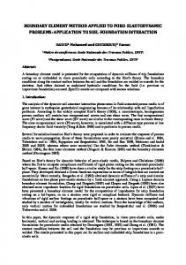
DUAL BOUNDARY ELEMENT METHOD FOR AXISYMMETRIC CRACK ANALYSIS
L. A. de Lacerda? and L. C. Wrobel† Brunel University, Department of Mechanical Engineering, Uxbridge, Middlesex UB8 3PH, UK. FAX: +44 1895 256392 ?
[email protected], †
[email protected] Short title : DUAL BEM FOR AXISYMMETRIC CRACK ANALYSIS
ABSTRACT In this paper a dual boundary element formulation is developed and applied to the evaluation of stress intensity factors in, and propagation of, axisymmetric cracks. The displacement and stress boundary integral equations are reviewed and the asymptotic behaviour of their singular and hypersingular kernels is discussed. The modified crack closure integral method is employed to evaluate the stress intensity factors. The combination of the dual formulation with this method requires the adoption of an interpolating function for stresses after the crack tip. Different functions are tested under a conservative criterion for the evaluation of the stress intensity factors. A crack propagation procedure is implemented using the maximum principal stress direction rule. The robustness of the technique is assessed through several examples where results are compared either to analytical ones or to BEM and FEM formulations. KEY WORDS: boundary element method, axisymmetry, fracture mechanics, modified crack closure integral method, Cauchy Principal Value, Hadamard Principal Value.
1
INTRODUCTION
Axisymmetric cracks are inherent from mechanical systems in which the geometry and loading conditions are symmetrical about an axial direction. Indentation tests, pressure vessels, pipes, are a few of the examples where such cracks might occur. The boundary element method has been applied to axisymmetric elasticity since the midseventies [1, 2, 3]. In structures where the crack is situated along a radial direction, symmetrically located with respect to the axial direction, application of the BEM is straightforward but limited to geometries satisfying this double symmetry condition [4, 5]. Chen and Farris [6] and more recently Selvadurai [7] and Bush [8] applied the BEM along with a multi-domain technique, which allowed the analysis of cracks at general orientations. The inconvenience of using the multi-domain technique is the need of introducing artificial discretizations connecting the crack tips to other boundaries. This drawback is clearly evident in crack propagation analysis [7, 8]. The dual BEM is an elegant approach for the analysis of crack problems [9, 10]. Its application to axisymmetric problems requires a stress (hypersingular) boundary integral equation together with the displacement (standard) boundary integral equation, one applied to each side of the crack. Recently, de Lacerda and Wrobel [11] derived such hypersingular equation, a process which involved a great amount of algebra due to the complexity of the axisymmetric kernels. The development of a dual BEM for the analysis of axisymmetric cracks is part of the proposal of the present work. The derivation of the standard and hypersingular boundary integral equations is reviewed and numerical aspects are discussed. The computation of stress intensity factors follows the work of Chen and Farris [6], who employed the modified crack closure integral method introduced by Rybicki and Kanninen [12] for finite element analysis. The method is based on the evaluation of Irwin’s [13] crack closure integral over the whole length of the tip element, and its main attraction is the accurate calculation of stress intensity factors even with coarse meshes. The possibility of combining this method with the dual BEM is investigated for a variable size of the integration path. Simple linear elements are used to discretize the crack and their performance is assessed through several examples. The material toughness and the maximum principal stress criteria are employed in the crack
propagation routines. An efficient approach is implemented using a predictor-corrector technique and an LU solver, as reported by Portela et al. [10]. The growth trajectories of a cylindrical crack are investigated under different load conditions.
2
AXISYMMETRIC STANDARD BIE Let a 2-D body B rotate 360 degrees about the z-axis, forming an axisymmetric geometry.
Under an axisymmetric load, all displacements and stresses are constant along the hoop direction, and this type of problem can be more efficiently analysed by simply considering the 2-D body B instead of the whole 3-D domain. As a result of this axisymmetry, directions r and z are sufficient to define the problem. The axisymmetric integral equation describing the problem is of the form ui (ξ) =
Z
Γ
λ(x)Uij (ξ, x)tj (x)dΓ −
Z
Γ
λ(x)Tij (ξ, x)uj (x)dΓ
(1)
with i, j = r, z, λ(x) = 2πrx , ξ is the point where the ring unit load is applied, x is the integrating field point, rx is the radial distance from the field point to the axis of symmetry, ur and uz are the radial and axial displacements, tr and tz are the radial and axial tractions, and U and T are the axisymmetric displacement and traction fundamental solutions which are functions of the complete elliptic integrals of the first (K1 ) and second kind (K2 ) [14]. The singular behaviour of kernels U and T is similar to their 2-D counterparts if the collocation point ξ is not at the axis of symmetry, 1 U 2D (ξ, x) + Uijr (ξ, x) λ(x) ij 1 Tij (ξ, x) = T 2D (ξ, x) + Tijw (ξ, x) λ(x) ij
Uij (ξ, x) =
O(ln R) O(R−1 )
(2)
where R = |x − ξ|, U 2D and T 2D are the 2-D displacement and traction fundamental solutions, and the terms U r and T w are the remaining parts of the axisymmetric kernels containing, at most, regular (r) and weak-singular (w) functions, respectively. When ξ is on the z-axis the ring load becomes a point load. The resultant of the load in the r-direction is zero; as a consequence, the components Urr , Urz , Trr and Trz of the kernels must also be zero. In the z-direction, it is easy to
verify that the components Uzr , Uzz , Tzr and Tzz reduce to the 3-D fundamental solutions, 3D Uzj (ξ, x) = Uzj (ξ, x)
O(R−1 )
3D Tzj (ξ, x) = Tzj (ξ, x)
O(R−2 )
(3)
However, due to the presence of the term λ(x) in the integrand and since ur (ξ) = 0, integration of Uzr , Uzz , Tzr and Tzz is bounded. In the limit, as ξ approaches the boundary Γ, the integral equation (1) must be analyzed when ξ is outside the axis of symmetry (case a) and when ξ is on the axis (case b). The following integral equation represents the transition of ξ from inside the domain onto the boundary as ε → 0, ui (ξ) = lim
Z
ε→0 Γ−Γ+Γε
λ(x)Uij (ξ, x)tj (x)dΓ − lim
Z
ε→0 Γ−Γ+Γε
λ(x)Tij (ξ, x)uj (x)dΓ
(4)
The first integral on the right-hand side of equation (4) reduces to a Riemman type of integral, for both cases a and b, since the integrand has at most a logarithmic singularity. Considering a Taylor expansion of the displacement field about the source point, the second integral reduces to a Cauchy Principal Value integral plus a free term Cij (ξ)uj (ξ). Finally, the displacement boundary integral equation writes [δij + Cij (ξ)]uj (ξ) =
Z
Γ
Z
λ(x)Uij (ξ, x)tj (x)dΓ − −λ(x)Tij (ξ, x)uj (x)dΓ
(5)
Γ
where δij is the Kronecker delta function and the sign on the second integral indicates Cauchy Principal Value. The free coefficient Cij (ξ), for case a, is given by Cruse et al. [3]. For case b only Czz (ξ) is relevant since the boundary integral equation reduces to ur (ξ) = 0 [1 + Czz (ξ)]uz (ξ) =
Z
Γ
Z
λ(x)Uzj (ξ, x)tj (x)dΓ − −λ(x)Tzj (ξ, x)uj (x)dΓ
with 1 Czz (ξ) = − − mr 2
(6)
Γ
Ã
4(1 − ν) − m2z 8(1 − ν)
!
(7)
where mr and mz are the components of the normal at the source point. Differentiating the displacement equation (1) with respect to directions r and z, substituting into the linear strain-displacement equations and these into Hooke’s law, the following integral
equation for stresses at interior points is obtained, σij (ξ) =
Z
Γ
λ(x)Dijk (ξ, x)tk (x)dΓ −
Z
Γ
λ(x)Sijk (ξ, x)uk (x)dΓ
(8)
with i, j, k = r, z, where the kernels D and S are given as functions of derivatives of U and T , and consequently, K1 and K2 [14].
3
AXISYMMETRIC HYPERSINGULAR BIE
The boundary integral equation for stresses is obtained applying the same limiting procedure previously described. Approaching ξ to the boundary Γ and making ε → 0 the stress integral equation writes, σij (ξ) = lim
Z
ε→0 Γ−Γ+Γε
Z
λ(x)Dijk (ξ, x)tk (x)dΓ − lim
ε→0 Γ−Γ+Γε
λ(x)Sijk (ξ, x)uk (x)dΓ
(9)
The exact singular behaviour of the fundamental solutions D and S is essential for the integral limit analysis. Their derivation involved a great deal of algebraic manipulation. Again, different expressions are applicable depending on the position of ξ. For simplicity, only case a is considered in this paper. A more comprehensive analysis can be found in [11]. D and S are composed by a sum of terms of different orders of singularity where the strongest singular terms for both fundamental solutions are similar to the plane 2-D ones, D2D and S 2D , Dijk (ξ, x) = Sijk (ξ, x) =
1 w (ξ, x) D2D (ξ, x) + Dijk λ(x) ijk
O(R−1 )
1 s w (ξ, x) + Sijk (ξ, x) S 2D (ξ, x) + Sijk λ(x) ijk
O(R−2 )
(10) (11)
where the two-dimensional fundamental solutions are given in [15] and the strong-singular terms, indicated by the superscript s, are given in [11]. The terms with superscript w in expressions (10) and (11) are regular or at most of a weak logarithmic singularity. Returning to equation (9), the first integral on the right-hand side can be subdivided in the form, lim
Z
ε→0 Γ−Γ+Γε
λ(x)Dijk (ξ, x)tk (x)dΓ = lim
Z
ε→0 Γε
lim
Z
λ(x)Dijk (ξ, x)tk (x)dΓ +
ε→0 Γ−Γ
λ(x)Dijk (ξ, x)tk (x)dΓ
(12)
Considering a Taylor expansion of the displacement derivatives about the source point, the first integral on the right-hand side becomes, lim
Z
ε→0 Γε
λ(x)Dijk (ξ, x)tk (x)dΓ = lim
Z
ε→0 Γε
lim
Z
ε→0 Γε
0
λ(x)Dijk (ξ, x)(tk (x)−tk (ξ, x))dΓ + 0
λ(x)Dkij (ξ, x)tk (ξ, x)dΓ
(13)
0
where the tractions tk (x) and tk (ξ, x) are expressed by tk (x) =
2µν 1 − 2ν
µ
and 2µν tk (ξ, x) = 1 − 2ν 0
¶
ur (x) + ul,l (x) nk (x) + µ (uk,l (x) + ul,k (x)) nl (x) rx
(14)
µ
(15)
¶
ur (ξ) + ul,l (ξ) nk (x) + µ (uk,l (ξ) + ul,k (ξ)) nl (x) rx
where nk (x) are the normal components at the field point. Assuming ur (x) and uk,l (x) as H¨oldercontinuous fields, the first integral on the right-hand side of equation (13) vanishes in the limiting process while the second produces a free term Aij (ξ) which is a function of the radial displacement, displacement derivatives and elastic properties. The second integral on the right-hand side of equation (12) is improper and must be calculated in the Cauchy Principal Value sense. Finally, the following result is obtained, lim
Z
ε→0 Γ−Γ+Γε
Z
λ(x)Dijk (ξ, x)tk (x)dΓ = −λ(x)Dijk (ξ, x)tk (x)dΓ + Aij (ξ)
(16)
Γ
Hypersingular, strong-singular, weak-singular and regular terms appear under the second integral of equation (9) which is expanded as, lim
Z
ε→0 Γ−Γ+Γε
λ(x)Sijk (ξ, x)uk (x)dΓ = lim
Z
2D Sijk (ξ, x)uk (x)dΓ +
lim
Z
s λ(x)Sijk (ξ, x)uk (x)dΓ +
ε→0 Γε
ε→0 Γε
lim
Z
ε→0 Γε
w λ(x)Sijk (ξ, x)uk (x)dΓ +
lim
Z
2D Sijk (ξ, x)uk (x)dΓ +
lim
Z
s w λ(x)(Sijk (ξ, x) + Sijk (ξ, x))uk (x)dΓ
ε→0 Γ−Γ
ε→0 Γ−Γ
(17)
The third integral on the right-hand side of equation (17) only contains weak-singular functions and vanishes once a polar coordinate transformation is applied. Considering two terms of the Taylor expansion of the displacement field, about the source point, the first integral on the right-hand side of equation (17) can be regularized, lim
Z
ε→0 Γε
2D Sijk (ξ, x)uk (x)dΓ
= lim
Z
ε→0 Γε
2D Sijk (ξ, x)(uk (x)−uk (ξ)−uk,m (ξ)Rm )dΓ +
uk (ξ) lim
Z
ε→0 Γε
uk,m (ξ) lim
2D Sijk (ξ, x)dΓ +
Z
ε→0 Γε
2D Sijk (ξ, x)Rm dΓ
(18)
Provided the displacement derivatives are at least H¨older-continuous, the first integral on the righthand side of equation (18) is not improper and vanishes in the limiting process. The second integral on the right-hand side produces the unbounded expression Bijk (ξ)uk (ξ)/ε and a second free term Fijk (ξ)uk (ξ) which depends on the curvature of the boundary at ξ and elastic properties [11, 16]. The last integral of equation (18) also produces a free term, Cijkm (ξ)uk,m (ξ), which also depends on elastic properties. Notice that the free coefficients Bijk (ξ), Fijk (ξ) and Cijkm (ξ) are the same for either 2-D or axisymmetric formulations. The fourth integral in equation (17) is improper and is evaluated in the Hadamard Principal Value sense along with the unbounded term. Their sum is represented by,
lim
Z
ε→0 Γ−Γ
2D Sijk (ξ, x)uk (x)dΓ +
Z
Bijk (ξ) 2D (ξ, x)uk (x)dΓ uk (ξ) = = Sijk ε
(19)
Γ
where the sign on the second integral indicates Hadamard Principal Value. It has been proved [16] that the unbounded term is always cancelled by another unbounded term arising from the integral. The first term of a Taylor expansion of the displacement field is also used for the analysis of the second integral on the right-hand side of equation (17). The limit can be written as lim
Z
ε→0 Γε
s λ(x)Sijk (ξ, x)uk (x)dΓ = lim
Z
ε→0 Γε
s λ(x)Sijk (ξ, x)(uk (x)−uk (ξ))dΓ +
uk (ξ) lim
Z
ε→0 Γε
s λ(x)Sijk (ξ, x)dΓ
(20)
Due to continuity properties of the displacement field the first integral on the right-hand side of equation (20) vanishes, while the second limit leads to a free term Eijk (ξ)uk (ξ), exclusive to the axisymmetric formulation, which is a function of elastic and geometric properties. The strongsingular terms in the integrand of the last integral of equation (17), requires its evaluation in the Cauchy Principal Value sense, while the weak-singular one is more easily treated, lim
Z
ε→0 Γ−Γ
Z
s w s λ(x)(Sijk (ξ, x) + Sijk (ξ, x))uk (x)dΓ = −λ(x)Sijk (ξ, x)uk (x)dΓ + Γ
Z
w λ(x)Sijk (ξ, x)uk (x)dΓ
(21)
Γ
The integral on the left-hand side of equation (17) is therefore, lim
Z
ε→0 Γ−Γ+Γε
λ(x)Sijk (ξ, x)uk (x)dΓ =
Z
2D = Sijk (ξ, x)uk (x)dΓ +
Γ
Z
s −λ(x)Sijk (ξ, x)uk (x)dΓ +
Γ
Z
w λ(x)Sijk (ξ, x)uk (x)dΓ +
Γ
Cijkm (ξ)uk,m (ξ) + Eijk (ξ)uk (ξ)+ Fijk (ξ)uk (ξ)
(22)
Finally, the stress boundary integral equation for axisymmetric problems with the source point outside the axis of symmetry reads, Z
Z
2D (ξ, x)uk (x)dΓ − σij (ξ) = −λ(x)Dijk (ξ, x)tk (x)dΓ − = Sijk Γ
Γ
Z
s −λ(x)Sijk (ξ, x)uk (x)dΓ −
Γ
Z
w λ(x)Sijk (ξ, x)uk (x)dΓ +
Γ
Aij (ξ) − Cijkm (ξ)uk,m (ξ) − Eijk (ξ)uk (ξ) − Fijk (ξ)uk (ξ)
(23)
and it can be verified that on a smooth boundary, Aij (ξ) − Cijkm (ξ)uk,m (ξ) − Eijk (ξ)uk (ξ) =
1 σij (ξ) 2
(24)
and also, if the curvature is continuous, Fijk (ξ) = 0
(25)
Multiplying both sides of equation (23) by mj leads to the traction equation Z
Z
1 2D (ξ, x)uk (x)dΓ − ti (ξ) = mj −λ(x)Dijk (ξ, x)tk (x)dΓ − mj = Sijk 2 Γ
Z
s mj −λ(x)Sijk (ξ, x)uk (x)dΓ − mj Γ
4
Γ
Z
w λ(x)Sijk (ξ, x)uk (x)dΓ
(26)
Γ
DUAL BEM AND NUMERICAL INTEGRATION
The dual BEM is an attractive method for the analysis of fracture mechanics problems. Compared to the multi-domain BEM, it has the advantage that discretizations are entirely restricted to the boundaries, which makes the computations more accurate. The analysis of crack propagation is also very efficient since remeshing is much easier. The dual boundary element method basically consists on the simultaneous application of the displacement and stress boundary integral equations to the crack boundaries [10], giving rise to a mathematically well-posed formulation. As seen in the previous section, in order to satisfy the continuity requirements for the displacement derivatives in the stress boundary integral equation, discontinuous linear elements are employed for the discretization of the cracks. Discontinuous elements have their edge nodes shifted towards the centre of the element, enforcing smoothness at the boundary nodes as well as continuity of displacement derivatives and boundary curvature at these points. Linear or quadratic isoparametric elements are used everywhere else. After the boundary discretization, equations (5) and (26) are applied at crack nodal points, one to each side of the crack. At non-crack boundaries either equation (5) or (6) is applied depending on the position of the source point ξ. A discretized system of equations is obtained where integrals over each element must be computed. Two types of integrations will appear, regular and singular. The first ones are computed using Gauss quadrature and the second requires different treatments, depending on which kernel of each equation is being integrated. Generally speaking, the singularity subtraction technique [17] is used to regularize the integrand of all Cauchy and Hadamard Principal Value integrals. In this procedure, the integrals are transformed into regular or weak-singular ones plus an improper integral suitable for evaluation by finite parts. Normal Gaussian integration is carried out for the regular integrals, while a local
coordinate transformation [18] along with Gaussian quadrature is employed in the evaluation of the weak-singular ones. For the source point outside the axis of symmetry, the boundary integral equations (5) and (26) can be expanded to [δij + Cij (ξ)]uj (ξ) =
Z
Γ
Uij2D (ξ, x)tj (x)dΓ +
Z
Z
Z
Γ
λ(x)Uijr (ξ, x)tj (x)dΓ −
−Tij2D (ξ, x)uj (x)dΓ − λ(x)Tijw (ξ, x)uj (x)dΓ Γ Γ
(27)
and
Z
Z
1 2D 2D (ξ, x)tk (x)dΓ − mj = Sijk (ξ, x)uk (x)dΓ − ti (ξ) = mj −Dijk 2 Γ
Γ
Z
s mj −λ(x)Sijk (ξ, x)uk (x)dΓ − mj Γ
mj
Z
Z
w λ(x)Sijk (ξ, x)uk (x)dΓ +
Γ
w λ(x)Dijk (ξ, x)tk (x)dΓ,
(28)
Γ
respectively. Evaluation of all improper integrals of 2-D functions is well described in the literature where direct [16, 10] or indirect [19, 20] methods may be applied. The present work uses the direct approach as reported by Portela et al. [10]. The third improper integral in equation (28) is new but its evaluation procedure follows the same approach. The exact singular behaviour of s (ξ, x) given by de Lacerda and Wrobel [11] is essential for this analysis. All integrands with Sijk
the superscript w are not explicitly known but they can be calculated by rearranging expressions (2), (10) and (11), Tijw (ξ, x) = Tij (ξ, x) −
1 T 2D (ξ, x) λ(x) ij 1 D2D (ξ, x) λ(x) ijk
(30)
1 2D s (ξ, x) S (ξ, x) − Sijk λ(x) ijk
(31)
w Dijk (ξ, x) = Dijk (ξ, x) − w (ξ, x) = Sijk (ξ, x) − Sijk
(29)
The use of a local coordinate transformation to cancel the logarithmic singularities requires extra w (ξ, x) which involves computation of terms of order R−2 . care, specially during integration of Sijk
The local transformation brings the Gauss points closer to the singular point. There is a range of
proximity to the singular point, dependent on the precision of the machine, from which inaccurate w (ξ, x). In order to overcome this problem, improper results are obtained when evaluating Sijk
integrations on crack elements are always divided into two subelements, one at each side of the singular node. A limited number of Gauss points is used for these subelements, in order to avoid this proximity. For the source point on the axis of symmetry, the boundary integral equation (6) writes, [1 + Czz (ξ)]uz (ξ) =
Z
Γ
3D λ(x)Uzj (ξ, x)tj (x)dΓ −
Z
3D −λ(x)Tzj (ξ, x)uj (x)dΓ
(32)
Γ
Integrations are straightforward if the boundary element being integrated does not contain ξ. If it does, apparently, singularity subtraction regularization is necessary in the last integral. However, 3D needs attention. since the radial displacement is equal to zero at the axis, only the kernel λ(x)Tzz
Expanding this kernel,
1 ∂R R ∂n(x)
3D (ξ, x) = λ(x)Tzz
µ
¶
´ −R,r ³ 2 (1 − 2ν) + 3R,z 4(1 − ν)
(33)
and since lim
R→0
1 ∂R 1 = R ∂n(x) 2ρ(ξ)
(34)
the last integral is in fact regular, thus it need not be regularized. Once the numerical integration is completed, a fully-populated system of equations My = b is finally obtained where y contains the unknown boundary values of displacements and tractions in directions r and z, M is the matrix of influence coefficients and b is the independent vector resulting from the multiplication of influence coefficients by their associated prescribed values. At a post-processing level, stresses at internal points are directly computed using equation (8) with no singularities in the integration since R > 0.
5
STRESS INTENSITY FACTORS
The relation between the stress intensity factors Ki and the strain energy release rate Gi , for an axisymmetric crack, is identical to the plane strain case and is given by, Ki =
s
E Gi 1 − ν2
i = I, II
G is defined as the work expended at the crack front to extend the crack a small increment of area δa. From an opposite direction, the strain energy release rate is also the work required to close the crack by the same amount δa. This idea provides the basis to the crack closure integral proposed by Irwin [13]. The formulas for modes I and II are GI
1 = lim δa→0 2δa
GII
1 = lim δa→0 2δa
Z
σn ∆un da
δa
Z
σt ∆ut da
(35)
δa
where σn and σt are the normal and tangential stresses along the path δa before the crack extension, and ∆un and ∆ut are the relative normal and tangential displacements at the path δa after the crack extension. The modified crack closure integral method [6, 12] is simply the approximate evaluation of integrals in expressions (35), taking displacements and stresses values for a single crack configuration. Rigorously, two analyses should be carried out. One with the crack length a where stresses would be calculated in an area δa just after the crack tip, and the second with the extended crack a + δa where displacements would be calculated in the same area. However, the displacement field just before the crack tip is very similar for both configurations and, as results will show, the proposed approximation seems very appropriate. Rybicki and Kanninen [12] using the finite element method and Chen and Farris [6] using a multi-domain boundary element method employed the nodal results of the elements adjacent to the tip, including the tip nodal result, to interpolate the displacements and stresses in the integrand of equations (35). Also, they considered the path δa to be equal to the tip element length. Apparently, the tip nodal finite value plays an important role in this method of analysis despite its lack of physical significance. In the dual boundary element method, stresses are calculated at a postprocessing level and they tend to infinity approaching the crack tip. A few tests were carried out using interpolating functions for the stresses which lead to an infinite value at the tip. In all cases, it was observed that the stress intensity factors were overestimated quite excessively, indicating that a large finite stress value at the tip should suffice to keep the crack closed. Based on this fact, tests were conducted combining the interpolating functions for the stresses and relative displacements in
tables 1 and 2, where r and r are defined in figure 1 and the constants αi are calculated according to the boundary nodes or internal points positions listed in the second column (see figure 1). The distances from the internal points 5, 6 and 7 to the crack tip are identical to the distances from the boundary nodes 3, 2 and 1 to the same point. Differently from previous applications of the modified crack closure integral method the path of integration is not fixed to the length of the tip element, but it varies from a small fraction of the element length to this upper limit. Gauss quadrature is used to perform the integration, and as a conservative criterion, the highest value of the strain energy release rate within this range is adopted for the computation of the stress intensity factors. The problem of a penny-shaped crack in an infinite medium under a uniform axial tensile stress was analysed in order to illustrate the behaviour of the different function combinations. The √ normalized stress intensity factor for this problem is KI /σ πa = 0.6366 [21] where σ is the applied stress and a is the crack radius. In figure 2, errors obtained from each combination of functions are plotted against the path length. In the legend, the first number between brackets indicates the displacement fitting function while the second indicates the stress one. Initially, 160 elements of size c were used in each face of the crack and results appear to be dependent on the length δa, but within 5% error provided δa > 0.4c. A smaller number of elements resulted in the same trend for the curves. It can also be seen that the adoption of the highest stress intensity factor criterion results in errors smaller than 1%, apart from cases (2)(1) and (2)(2). The convergence of results using the previous criterion is clearly evident from figure 3 as the number of elements is increased from 2 to 160. Again, apart from cases (2)(1) and (2)(2), less than 1% error was achieved with 40 elements. Perhaps it is more remarkable that errors were smaller than 8% even when only two boundary elements were applied in each crack face, confirming the possibility of achieving reasonably good results using coarse meshes [6, 12]. It is not possible to point out which combination of functions is the best since results will change for different problems. For simplicity, combination (1)(1) with 40 discontinuous linear boundary elements in each side of the crack is adopted in all analyses of the next section, unless otherwise stated.
6
CRACK PROPAGATION
If the stress intensity factor (K) is higher than the toughness (T ) of the material the crack will grow until K < T . In the following tests T is set equal to zero since its value does not affect the crack trajectories, although it will have an influence on the load level at which cracks will start propagating. The maximum principal stress criterion is used to calculate the crack growth direction. This criterion predicts that the crack will grow perpendicularly to the principal stress direction at the crack tip. Knowledge of KI and KII is sufficient to calculate this direction using the expression −1
θ = 2 tan
· µ
¶¸
q 1 f + f2 + 8 4
,
f = KI /KII
where θ is measured from the crack axis ahead of the crack tip. Once the growth direction is defined, a crack increment is added to the system: one pair of boundary elements with length comparable to the tip element size. This procedure constitutes an extremely easy re-meshing approach. Moreover, the added pair of elements only contributes with a few extra rows and columns to the global system of equations, so their assembling is very fast. Notice that the predicted angle does not take into account the length of the increment, so a correction is necessary to adjust this orientation. This predictor-corrector technique is an iterative procedure which can be used very efficiently with the dual boundary element method and an LU solver [10].
7
EXAMPLES
Different types of axisymmetric cracks in a cylinder are analysed and compared to available results. Non-dimensional material properties are used in all cases. Penny-shaped crack Consider a cylinder with radius b = 1.0, infinite height H and material properties E = 20000 and ν = 0.3, subjected to a tensile axial stress σ = 1.0. The cylinder contains a penny-shaped crack with radius a perpendicular to the axis of symmetry at mid-height position. An analytical solution
was developed by Benthem and Koiter [23] based on asymptotic approximations, √ µ ¶ KI 1−λ 1 2 3 √ = (2 + λ − 1.25λ ) + 0.268λ , λ = a/b σ πa 1 − λ2 π In this analysis, a value of H = 6.0 was verified to be large enough to simulate the infinite length and despite the double symmetry condition, discretization was performed at the whole cylinder (apart from the axis of symmetry). Figure 4 displays the relative differences between the previous formula and the dual boundary element method. A very close agreement can be seen with differences of less than 1% for a/b ≤ 0.8, but the difference tends to increase as the crack radius approaches the cylinder radius. A similar trend has been reported by Miyazaki et al. [5] using boundary elements combined with an energy method. A similar problem, with H = 2.8 and a = 0.5, has been analysed by Leung and Su [22] using a two-level finite element method, and by Chen and Farris [6] using a multi-domain boundary element method. Results for the normalized stress intensity factors are compared in table 3, where the number of elements applied to each crack face is indicated between brackets. They appear to converge to a value closer to the two-level finite element result, in contrast to the multi-domain BEM. As previously mentioned, results are quite good even for coarse meshes. Circumferential edge crack Consider an infinite cylinder with the same radius, material properties and applied stress as before, with a horizontal edge ring crack at mid-height position. Benthem and Koiter [23] also developed an asymptotic solution for this problem, ³ ´ K 1 √ I = λ−3/2 1 + 0.5λ + 0.375λ2 − 0.363λ3 + 0.731λ4 , σ πa 2
λ=
b−a b
The relative differences between their formula and the dual boundary element method are plotted in figure 5 for several values of the crack size a. Differences appear to be larger than in the previous example but with the same increasing trend as a approaches the cylinder radius. Solutions from other authors for a similar problem with H = 2.8 and a = 0.5 are listed in table 4. The present method seems to converge to a value closer to Hellen’s [24] who used quadratic finite elements with special crack tip elements, and to Becker’s [14] who used boundary elements with singular crack tip elements.
Cylindrical crack In this test, a cylindrical crack is located at the mid-height interior of a large cylinder of radius b = 20a and height H = 20a. The longitudinal axes of the crack and cylinder are coincident and a radial tensile stress σ was applied to the cylinder. Here, the double symmetry of the problem is taken into account and only a quarter of the model (considering plane rz) is discretized. Figure 6 √ shows the computed modes I and II normalized stress intensity factors (KI,II / σ πa) for several d/a and Poisson’s ratios, where d is the radius of the cylindrical crack. No alternative numerical data is available for comparison, but a very similar plot was presented by Chen and Farris [6] who analysed the same problem for ν = 0.3. Analytical expressions have been derived by Demir et al. [25] for a pressurized cylindrical crack in an infinite medium. Although boundary conditions are not the same, their results are visually quite close to the present ones. Cone crack The final test simulates the propagation of a branched cone crack inside a large cylinder for different static loading conditions: a) axial unit load, b) radial unit load and c) both simultaneously applied. The cylinder dimensions are radius b = 40a and height H = 40a, with initial crack length a = 1. Material properties are E = 20000 and ν = 0.3. The cone crack is at 45◦ and the ratio d/a is set equal to 4, with d in this case representing the radius of the base of the cone crack (figure 7). The discretization employed continuous quadratic elements, with 40 and 20 elements located at the top and at the side of the cylinder, respectively. At the crack, 10 equal discontinuous quadratic elements were initially located on each face. The resulting crack trajectory for each load case is shown in figure 7, for a total of 60 crack increments. At each increment, the crack propagates by one element of the same type and size of those used to discretize the initial crack. The bending of the crack away from the symmetry axes for load cases a) and b) is due to the interaction between the cracks that form the respective cones. Although similar previous analysis could not be found for comparison, it is clear that the present results are consistent with each applied load. Table 5 presents the results of a convergence study of the crack trajectory for loading case c) above. The table shows the position of the crack tip when using 5, 10 or 20 elements to discretize
the initial crack. Since the crack propagates by one element per increment, the corresponding total number of increments for each case are 30, 60 and 120, respectively. The results in the table confirm the convergence and accuracy of the proposed dual BEM formulation.
8
CONCLUSIONS
The dual boundary element method has been developed and successfully applied to axisymmetric crack problems. The standard and hypersingular boundary integral equations were presented along with their corresponding fundamental solutions. The exact hypersingular and strong-singular behaviour of the integral kernels was derived allowing the application of the singularity subtraction technique for the evaluation of the Hadamard and Cauchy Principal Value integrals. Details of the singular integrations were shown where a variable number of Gauss points was used in order to avoid integration errors. The use of the modified crack closure integral method combined with the dual BEM for the computation of stress intensity factors was assessed. Several types of interpolating functions for the stresses and relative displacements were used with a variable size of the integration path. The highest stress intensity factor within this variable range was adopted as the final result. Results were generally good for all choices of interpolating functions, despite using linear elements, and the simplest case was selected for the remaining tests. Different axisymmetric cracks were analysed and results compared to available numerical and analytical solutions. Very accurate results were obtained in all cases. An efficient crack propagation simulation was implemented and results from a test case were shown to be convergent and consistent with the applied loading.
References [1] Kermanidis, T. (1975). A numerical solution for axially symmetrical elasticity problems, International Journal of Solids and Structures, 11, 493-500. [2] Mayr, M. (1976). The numerical solution of axisymmetric elasticity problems using an integral equation approach, Mechanics Research Communication, 3, 393-398.
[3] Cruse, T., Snow, D. W. and Wilson, R. B. (1977). Numerical solutions in axisymmetric elasticity, Computers & Structures, 7, 445-451. [4] Bakr, A. A. and Fenner, R. T. (1985). Axisymmetric fracture mechanics analysis by the boundary integral equation method, International Journal of Pressure Vessels and Piping, 18, 55-75. [5] Miyazaki, N., Ikeda, T. and Munakata, T. (1989). Analysis of stress intensity factor using the energy method combined with the boundary element method, Computers & Structures, 33, 867-871. [6] Chen, S. Y. and Farris, T. N. (1994). Boundary element crack closure calculation of axisymmetric stress intensity factors, Computers & Structures, 50, 491-497. [7] Selvadurai, A. P. S. (1998). The modelling of axisymmetric basal crack evolution in a borehole indentation problem, Engineering Analysis with Boundary Elements, 21, 377-383. [8] Bush, M. B. (1999). Simulation of contact-induced fracture, Engineering Analysis with Boundary Elements, 23, 59-66. [9] Gray, L. J., Martha, L. F. and Ingraffea, A. R. (1990). Hypersingular integrals in boundary element fracture mechanics, International Journal for Numerical Methods in Engineering, 29, 1135-1158. [10] Portela, A., Aliabadi, M. H. and Rooke, D. P. (1991). The dual boundary element method: effective implementation for crack problems, International Journal for Numerical Methods in Engineering, 33, 1269-1287. [11] de Lacerda, L. A. and Wrobel, L. C. (2001). Hypersingular boundary integral equation for axisymmetric elasticity, International Journal for Numerical Methods in Engineering, 52, 13371354. [12] Rybicki, E. F. and Kanninen, M. F. (1977). A finite element calculation of stress intensity factors by a modified crack closure integral, Engineering Fracture Mechanics, 9, 931-938. [13] Irwin, G. R. (1957). Analysis of stresses and strains near the end of a crack traversing a plate, Journal of Applied Mechanics, 24, 361-364.
[14] Becker, A. A. (1986). The Boundary Integral Equation Method in Axisymmetric Stress Analysis Problems, Springer-Verlag, Berlin. [15] Brebbia, C. A., Telles, J. C. F. and Wrobel, L. C. (1984). Boundary Element Techniques, Springer-Verlag, Berlin. [16] Guiggiani, M. (1995). Hypersingular boundary integral equations have an additional free term, Computational Mechanics, 16, 245-248. [17] Davis, P. J. and Rabinowitz, P. (1984). Methods of Numerical Integration, Academic Press, New York. [18] Telles, J. C. F. (1987). A self-adaptive co-ordinate transformation for efficient numerical evaluation of general boundary element integrals, International Journal for Numerical Methods in Engineering, 24, 959-973. [19] Lutz, E. D., Gray, L. J. and Ingraffea, A. R. (1990). Indirect evaluation of surface stress in the boundary element method, Proceedings of IABEM’90, Rome. [20] Krishnasamy, G., Schmerr, L. W., Rudolphi, T. J. and Rizzo, F. J. (1990). Hypersingular boundary integral equations: some applications in acoustic and elastic wave scattering, ASME Journal of Applied Mechanics, 57, 404-414. [21] Sneddon, I. N. (1946). The distribution of stress in the neighborhood of a crack in an elastic solid, Proceedings of the Royal Society of London A, 187, 229-260. [22] Leung, A. Y. T. and Su, R. K. L. (1998). Two-level finite element study of axisymmetric cracks, International Journal of Fracture, 89, 193-203. [23] Benthem, J. P. and Koiter, W. T. (1973). Asymptotic Approximations to Crack Problems in Mechanics of Fracture, Ed. by G. C. Sih, Noordhoff, Leyden, 131-178. [24] Hellen, T. K. (1976). Finite Element Energy Methods in Fracture Mechanics, Ph.D. Thesis, University of London.
[25] Demir, I., Hirth, J. P. and Zbib, H. M. (1992). The extended stress field around a cylindrical crack using the theory of dislocation pile-ups, International Journal of Engineering Science, 30, 829-845.
stresses σ(1) = α0 + α1 r σ(2) = α0 + α1 r + α2 r2
internal points 5 and 6 5, 6 and 7
Table 1: Interpolating functions for stresses relative displacements ∆u(1) = α0 + α1 r ∆u(2) = α0 + α1 r + α2 r2 ∆u(3) = α0 + α1 r + α2 r2 + α3 r3 √ ∆u(4) = r − α0 (α1 + α2 r) √ ∆u(5) = r − α0 (α1 + α2 r + α3 r2 )
boundary nodes 2 and 3 2, 3 and 4 1, 2, 3 and 4 2, 3 and 4 1, 2, 3 and 4
Table 2: Interpolating functions for relative displacements KI √ σ πa
Dual BEM (5 elements) Dual BEM (10 elements) Dual BEM (20 elements) Dual BEM (40 elements) Dual BEM (80 elements) Dual BEM (160 elements) Leung and Su [22] Chen and Farris [6] Benthem and Koiter [23]
0.714 0.700 0.693 0.689 0.687 0.686 0.685 0.700 0.688
Table 3: Comparison of results for a penny-shaped crack in a cylinder KI √ σ πa
Dual BEM (5 elements) Dual BEM (10 elements) Dual BEM (20 elements) Dual BEM (40 elements) Dual BEM (80 elements) Dual BEM (160 elements) Hellen [24] Leung and Su [22] Becker [14] Benthem and Koiter [23]
2.011 1.984 1.966 1.955 1.948 1.944 1.941 1.901 1.933 1.901
Table 4: Comparison of results for a circumferential edge crack in a cylinder
number of elements in initial crack 5 10 20 5 10 20 5 10 20
increment
r
z
10 20 40 20 40 80 30 60 120
5.266 5.260 5.258 6.116 6.118 6.120 7.332 7.340 7.345
2.627 2.628 2.629 4.432 4.430 4.429 6.016 6.009 6.006
Table 5: Position of the crack tip at different increments for cone crack in large cylinder
(i))
∆u ∆u1
σ
∆u2 1
σ5 ∆u3
2
δa
4 3 tip 5
r
(i))
σ6 6
σ7 7
0
r = δa - r
crack elements
internal points
Figure 1: Crack tip discretization and internal points for the evaluation of stress intensity factors.
Relative error in normalized KI (%)
3.0 (1)(1) (2)(1) (3)(1) (4)(1) (5)(1)
2.0 1.0
(1)(2) (2)(2) (3)(2) (4)(2) (5)(2)
0.0 -1.0 -2.0 -3.0 -4.0 -5.0 0
0.2
0.4
0.6
0.8
1
δa / c
Figure 2: Relative error for the normalized stress intensity factor using several stress and displacements interpolating functions and 0 < δa ≤ c.
Relative error in normalized KI (%)
8.0 7.0
(1)(1) (2)(1) (3)(1) (4)(1) (5)(1)
6.0 5.0 4.0
(1)(2) (2)(2) (3)(2) (4)(2) (5)(2)
3.0 2.0 1.0 0.0 -1.0 -2.0 0
40
80
120
160
Number of elements
Figure 3: Convergence of the normalized stress intensity factors with the increasing number of elements applied to each crack face.
Relative differences in normalized KI (%)
2.5 2
(1)(1) 1.5 1 0.5 0 -0.5 0
0.1
0.2
0.3
0.4
0.5
0.6
0.7
0.8
0.9
1
a/b
Figure 4: Relative differences, in the normalized stress intensity factor of a penny-shaped crack, between the dual boundary element method combined with the modified crack closure integral method and the analytical formula due to Benthem & Koiter [23].
Relative differences in normalized KI (%)
7.0 6.0
(1)(1)
5.0 4.0 3.0 2.0 1.0 0.0 0
0.1
0.2
0.3
0.4
0.5
0.6
0.7
0.8
0.9
1
a/b
Figure 5: Relative differences, in the normalized stress intensity factor of a circumferential edge crack, between the dual boundary element method combined with the modified crack closure integral method and the analytical formula due to Benthem & Koiter [23].
Normalized stress intensity factors
1 0.8
KI
ν
0.6
0 0.3 0.5 0
0.4 0.2
KII
0 -0.2 0
2
4
6
8
10
d/a
Figure 6: Normalized stress intensity factors of a cylindrical crack inside a large cylinder under tensile radial stress.
Figure 7: Crack propagation of a cylindrical crack inside a cylinder under three different loading conditions: a) axial unit load, b) radial unit load and c) both simultaneously applied.