1
Dynamic and Flexible Vision of a Spatial Database
Claramunt C.(1)
Mainguenaud M.(2)
(1) Swiss Federal Institute of Technology Rural Engineering Department CH1015 Lausanne, Switzerland Email:
[email protected] Fax: + 41 21 693 37 39 (2) France Telecom - Institut National des Télécommunications 9 rue Charles Fourrier F91011 Evry, France Email:
[email protected] Fax: + 33 1 60 77 20 06
Abstract: Today geographical databases must provide a dynamic and flexible data model. The notion of spatial view allows different, independent external interpretations of a database schema. A spatial view is an extension of the classical view concept as found in relational databases. A spatial view is a set of atoms. Each atom is defined with a set of database relations, a set of conventional spatial and non spatial database operators and a set of visualization operators. Manipulations of views allow building of new views according to specific needs.
Key words: Geographical Information System, Spatial Database, View
I. INTRODUCTION In current research toward the design of more powerful tools for urban planning and remote sensing, different groups are simultaneously concentrating their work on Geographical Information Systems (GIS). GIS needs are very well known [10]. Nevertheless, several problems are still open. Sharing data between several users is one of the most important issues to deal with in the design of spatial databases (e.g., accuracy and quality of data). A database system must provide a dynamic and flexible data model to take into account several requirements (eventually in contradiction with one another). The view mechanism allows the representation of alphanumeric data according to a point of view and in function of objectives which may be different from those of the database schema. The role of a view may be defined as a flexible and evolutive representation; flexible in that it allows the user to choose the appropriate representations and evolutive because a view contributes to a correct
2 cohabitation of database schema and applications over time. Unfortunately, no view definition has been offered for spatial data (see [5] for related work). This paper proposes the definition of a view formalism for spatial databases. This proposal is defined as an extension of the relational view mechanism (i.e., from the database point of view and not from the cartographer's point of view). The relational model [12] is well known and provides a vehicle to present our ideas. Nevertheless an object oriented formalism could have been used. Spatial views are modelled with an Abstract Data Type formalism which allows the representation of alphanumeric and spatial data. A Spatial View is a set of atoms. Each atom is defined with a set of database relations, a set of conventional spatial and non spatial database operators and a set of visualization operators. View operators are defined as functions on ADT. They allow the building of new views according to specific needs. Part II presents a database used to illustrate the view formalism; Part III, the Spatial View concept; Part IV, the Spatial View operators; Part V, a conclusion. II. EXAMPLE DATABASE A definition of a GIS database requires a study in three steps. The first step is the definition of a model for alphanumeric data. The second step is a definition of a model for spatial data. The third step is the merge of these two models into a unique formalism. II.1. Modelling of alphanumeric data We do not attempt to define a new model of alphanumeric data as this is beyond the scope of this paper. Alphanumeric data are well adapted to a top-down analysis. To simplify the presentation1, let us use the relational data model with the ANSI/SPARC proposition in three steps: alphanumeric external level, alphanumeric conceptual level and alphanumeric internal level. II.1.1. Alphanumeric external level Aside from security concerns, the external level allows the creation of a personalized collection of relations, a view, that is better matched to a certain intuition than is the conceptual model. The external level describes the viewpoint of specific groups of database users. Let us define two users U1 and U2. Figure II.1 presents a toy database schema for user U1. Figure II.2 presents a toy database schema for user U2.
1 Several simplifications are introduced, nevertheless they do not imply a loss of generality.
3 Forest Town
(Name, Trees) (Name, Active_Population) Figure II.1 - Database model for user U1
Flight Forest Town
(Name, Origin, Destination, Price) (Name, Trees) (Name, Main_Activity) Figure II.2 - Database model for user U2
II.1.2. Alphanumeric conceptual level The conceptual level provides a machine-independent, high-level representation of the whole database. This level is the synthesis of the different views. To simplify, we do not mention here the spatial semantics of alphanumeric attributes [7] and we do not consider here the mechanisms to provide such a conceptual data model (e.g., view integration [2]). Let us only consider the result of such a process. Figure II.3 presents the toy conceptual database. Flight Forest Town
(Name, Origin, Destination, Price) (Name, Trees) (Name, Activity, Population_in_this_Activity) Figure II.3 - Conceptual database
A relation of this database is called a theme (e.g., a town). A tuple of these relations is called a geographical object (e.g., a town called Paris). A user defined view is obtained from the conceptual database with a query. Figure II.4 presents the definition of the Town relation for each user (U1 and U2). Select From Group by Select From Where
Name, Sum (Population_in_this_Activity) Town Name
T1.Name, T1.Activity Town T1 Activity in ( Select T2.Activity From Town T2 Where T1.Name = T2.Name and T2.Population_in_this_Activity = ( Select Max (Population_in_this_Activity) From Town T3 Where T3.Name = T2.Name Figure II.4 - Town relation for users U1 and U2
) )
4 Figure II.5 presents a set of geographical objects for this conceptual database. TOWN
FOREST
Name
Activity
Pop_in_this_Activity
Paris
Tourism
500 000
Paris
Industry
100 000
Nice
Tourism
300 000
Lyon
Industry
350 000
Name
Trees
Name
Origin
Destination
Price
Vincennes Oak
AF101
Lyon
Nice
100
Boron
IT502
Paris
Lyon
150
AF303
Nice
Paris
120
AF204
Paris
Nice
140
Pine
Tête d'Or Fir
Flight
Figure II.5 - Instances of the conceptual database II.1.3. Alphanumeric internal level The internal level provides a machine-dependent description of the physical implementation of the database. This step is an important part of database design when there is a huge amount of data. The goal of a DBMS is to simplify and facilitate access to data. The conceptual model of the database is the correct level for database users to focus on. Users of the system should not be burdened unnecessarily with the physical details of the implementation of the system. The purpose of this section is to define an alphanumeric data model to be manipulated by end-users. Therefore, we do not consider this level. II.2. Modelling of spatial data We do not attempt to define a new spatial data model, as this is beyond the scope of this paper. Let us use the notion of Abstract Data Types [11]. Basic rules [1] to construct a type are as follows: (1) We assume that we are given a countable set of attribute names (ai). (2) We assume that attributes names can be unambiguously recognized from any other types in the system. (3) Types are defined recursively as follows: . Integer, float, string and Boolean are types (we call them atomic types) . If T1, ..., Tn are types and a1, ..., an are distinct attributes names then T = [a1:T1, ..., an:Tn] is a type (we call it a tuple type) . If T1 is a type: T = {T1} is a type.
5 . If T1 is a type: T = (T1, ..., Tn) is a type. . If T1 is a type: T = is a type. A spatial representation is associated with a theme. To simplify the presentation, let us consider the study of a unique spatial representation for all the themes. Historically, spatial data are studied with a bottom-up analysis. To present a model of spatial data, we use a three steps decomposition: internal spatial level, conceptual spatial level and external spatial level. II.2.1. Internal spatial level The internal level provides a worldwide coordinate-dependent description of spatial data. Several propositions have been made to handle physical representation of geographical data. They are based mainly on a vector or a raster representation [9]. To simplify the presentation, let us consider a spatial Abstract Data Type, called Representation_type, is available. This type is able to handle a physical representation of a spatial object (point, line, area, enclave, exclave, etc.). Figure II.6 presents the model of a spatial representation. Spatial_Representation_type = [
Cartographic_Representation : Representation_type
]
Figure II.6 - Spatial_Representation_type type Figure II.7 presents the spatial representations for geographical objects presented in Figure II.5.
Paris
AF204 AF303
IT502 Nice
Vincennes Tête d'Or
Lyon
Boron AF101
Figure II.7 - Spatial representation of the example database
6 II.2.2. Conceptual spatial level Let us define several components for the conceptual spatial level. These components are called Observation_Scale, Validity_Scale, Significant_Scale, Mode and Visualization. They complete the Spatial_Representation_type type. Observation_Scale The Observation_Scale property specifies the spatial referencing scheme or the perception level of a phenomenon (i.e., global, regional, local) within which a physical representation is defined. We can observe that GIS users share and use common observation scales. The Observation_Scale property defines the representation level of spatial data. Validity_Scale The Validity_Scale property defines a scale of validity for a physical representation. To illustrate this notion, let us consider the interval of relevant scales associated with a spatial representation as a reference. This interval is defined by the self-explanatory attributes Minimum_Scale, Maximum_Scale and Scale_Capture (i.e., the "best" validity scale for graphical representation).
Significant_Attributes The Significant_Attributes property completes the previous definitions. It specifies and references semantically relevant alphanumeric attributes for this observation scale. Mode A visualization of a geographical object may be realized from two cartographic primitives types: real and virtual [8]. "Real" cartographic primitives correspond to a geometric space reality and are significant for a geographical object. "Virtual" cartographic primitives are not geometrically significant (e.g., a schematic limit). A spatial operation is generally efficient if it is performed from real cartographic primitives. Conversely, virtual representations do not guarantee the quality of the result of a spatial operation. However, a virtual representation may be used for approximate spatial operations in the case of complex or large databases, where it provides a preliminary evaluation result.
7 Visualization Visualization processes are a function of spatial representations and particularly of the different cartographic primitive levels. A legend is a system of graphic symbols such as pictographic symbols or geometric symbols and a label. The type of symbolism varies with map scale, pattern complexity and intended audience. Visualization parameters (e.g., pattern) are classified and referred to as Bertin variables [3]. Let Bertin_Variables_type be the type which models such parameters. A label identifies a theme involved in the visualization process. If a geographical object has at least two physical representations, the corresponding geographical object has a multi-valued physical representation, or, in other word, a multiple spatial representation. A geographical object may have many physical representations for a considered scale if their scale validity intervals overlap. In this case, a geographical object has multiple interpretations for the same scale (e.g., two different user "views" for the same object). Figure II.8 presents the ADT model of the conceptual level of a Spatial_Representation_type type. For the time, we consider a list since the operator of cartographical generalization is far from being available. Spatial_Representation_type = ( [ Cartographic_Representation : Representation_type, Observation_scale : , Validity_Scale : [ Minimum_Scale : float, Maximum_Scale : float, Scale_Capture : float ], Significant__Attributes : { string }, Mode : , Visualization : [ Visualization_Function : Bertin_Variables_type, Label : string ] ] ) Figure II.8 Spatial_Representation_type type II.2.3. External spatial level The aim of the external spatial level is similar to the aim of the alphanumeric external level. An end-user may require a personalized Spatial_Representation_type for a given theme. Figure II.9 (respectively Figure II.10) presents the Spatial_Representation_type type for user U1 (respectively user U2).
8 Spatial_Representation_type = ( [ Cartographic_Representation : Representation_type, Observation_scale : , Validity_Scale : [ Minimum_Scale : float, Maximum_Scale : float, Scale_Capture : float ], Significant__Attributes : { string }, Visualization : [ Visualization_Function : Bertin_Variables_type, Label : string ] ] ) Figure II.9 - Spatial_Representation_type type for user U1 Spatial_Representation_type = ( [ Cartographic_Representation : Representation_type, Validity_Scale : float, Mode : , Visualization : [ Visualization_Function : Bertin_Variables_type, Label : string ] ] ) Figure II.10 - Spatial_Representation_type type for user U2
II.3. Conclusion The merge of an alphanumeric model and a spatial data model provides a unique conceptual database model with an ADT. Figure II.11 presents the conceptual database model (with normalized relations). Town Town_Representation Forest Flight
(Name, Activity, Population_in_this_Activity) (Name, Spatial_Representation) (Name, Trees, Spatial_Representation) (Name, Origin, Destination, Price, Spatial_Representation) Figure II.11 - Conceptual data model
The definition process of the spatial external level is similar to the definition process of the alphanumeric external level. A Data Definition Language (DDL) such as SQL is well adapted to handle these definition processes since the semantics are the same (e.g., a sub set of properties or a restructuring of relations or ADT and an extension to ADT).
9 Figure II.12 (respectively Figure II.13) presents the external database model for user U1 (respectively U2). We can note that the Spatial_Representation attribute may be defined for different domains depending on the themes. Forest Town
(Name, Trees, Spatial_Representation) (Name, Active_Population, Spatial_Representation) Figure II.12 - Database model for user U1
Flight Forest Town
(Name, Origin, Destination, Price, Spatial_Representation) (Name, Trees, Spatial_Representation) (Name, Main_Activity, Spatial_Representation) Figure II.13 - Database model for user U2
III. SPATIAL VIEW CONCEPT A Spatial View Atom (SVA) is designed as the application of spatial and non spatial manipulation operators (OM) combined with visualization operators (OV) on one or many collections -i.e., relations- (C). Each triplet [{OM}, {OV}, {C}] defines a Spatial View Atom. A Spatial View (SV) is a set of SVA. III.1. Spatial and non spatial operators A combination of spatial and non spatial operators defines a query. Several sets of spatial operators have been proposed to query geographical databases. Extending a DBMS with spatial operators implies the definition of a core of operators to respond to spatial manipulation needs. Providing such a framework is very difficult and sometime application-dependent. We are only concerned with the management of GIS query results but not the way of obtaining theses results. To simplify, let us retain only one spatial operator: intersection (∩) and its associated predicate: the intersection (∩T/F). Non spatial operators are provided to manage alphanumeric data. Let us use a subset of relational operators: the selection and the projection. To simplify the presentation, let us use an Extended SQL-like query language to define a combination of spatial and non spatial operators.
10 III.2. Visualization operators Many authors propose visualization operators for spatial information that may be logically inserted into a Select clause of a SQL statement [4]. A brief overview aims to illustrate our purpose while defining a set of visualization operators. Let us define three classes of operators as an example. Generalization operators are defined as simplification, smoothing, aggregation, amalgamation, merging, collapse, refinement, exaggeration, enhancement or displacement. Thematic classification is defined according to cartographic methods. Context display of geographical queries is handled with a background, a legend (i.e., an Update_Legend function) and a scale display [6]. To simplify the presentation, let us retain a unique function defined on a legend. Let us define the Update_Legend function with the following signature: Update_Legend : Spatial_Representation_type x Bertin_Variables_type x string -> Spatial_Representation_type where Bertin_Variables_type and string represents the manipulation of a component defined in the Bertin_Variables_type type (e.g., pattern, half_point). III.3. Collections An external database schema is a set of collections (i.e., database relations). These relations (e.g., Town and Forest for user U1) are transformed into a set of Spatial View Atoms. A database relation is defined as a Spatial View Atom with an empty set of spatial and non spatial operators and an empty set of visualization operators. III.4. Spatial View Human perception of graphic information is limited by visual acuteness and size limitations of a graphic interface, especially in the case of complex queries. Moreover, when the scale is reduced, linear entities are overestimated with respect to polygonal geographical objects, or visualized classes may be reduced and the visual density may increase. These progressive and interrelated phenomena have to be controlled to ensure the quality of visualization results. The Spatial View concept is a preliminary attempt to link human perception of space with a database query language. A Spatial View is designed to be used as the context of a geographical query. Its main advantage over manipulations with a query language is to free the user from specifying a display (since data are shared by different users who may have different objectives). A Spatial View groups Spatial View Atoms together. Spatial View Atoms are closed under their definition (i.e., a Spatial View Atom is defined with Spatial View Atoms). A relational view is designed to be used as a relation. Nevertheless, a Spatial View is not a relation but a set of relations.
11 A Spatial View Atom or a Spatial View is identified with a name. Let Name_type be the type which models this name. The different visualization collections are semantically and cartographically interdependent. Visualization objects may be ordered by relative semantic importance and relative query roles. This can be seen as an answer to both application objectives and the progressive saturation of a display space query. The respective contribution of each Spatial View Atom may be consequently analyzed depending on the query semantics with respect to user and application objectives. We can distinguish three levels of importance for Spatial View Atoms: - directly involved in the query result (essential); - used within the query (important); - used as background maps (useful). We represent this classification within the Spatial View definition by an order attribute that manages the relative importance of different Spatial View Atoms (essential, important, useful). Each Spatial View is additionally defined by a visualization scale (bounded and referenced) which is specified by a visualization scale attribute. This attribute provides a filter on the Validity_Scale attributes of the different SVA belonging to this Spatial View. A Spatial View is defined as presented in FigureּIII.1.
Spatial_View_Atom_type = [ Name : Name_type, Collection : {string}, Operators : { string }, Visualization_Operators : { string } ] Order_type = [
Essential : {Spatial_View_Atom_type}, Important : {Spatial_View_Atom_type}, Useful : {Spatial_View_Atom_type} ]
Elementary_Construction_Scale_type [ Minimum_Limit : float, Scale_Display : float, Maximum_Limit : float ]
=
Construction_Scale_type = { Elementary_Construction_Scale
}
Spatial_View_type = [ Name : Name_type, Order : Order_type, Construction_Scale : Construction_Scale_type ] Figure III.1 - Definition of a Spatial View
12 III.5. Example Let us define five Spatial View Atoms for user U2 to illustrate the notion of Spatial View. The first SVA represents the forest part of a town with tourism as its main activity. A relational view is defined with a query. The definition of a SVA follows the same approach. Figure III.2 presents the definition of this SVA. Name : SVA Forest_in_Town (Name_Forest, Name_Town, Spatial_Representation) Collection : {Forest, Town} Operators : {Select F.Name, T.Name, ∩ (F.Spatial_Representation,T.Spatial_Representation) From Forest F, Town T Where T.Main_Activity = 'Tourism' and ∩T/F (F.Spatial_Representation, T.Spatial_Representation)} Visualization_Operators : {Update_Legend (Spatial_Representation, pattern, half_point)} Figure III.2 - SVA Forest_in_Town The second SVA handles the spatial representation of relevant forests of SVA Forest_in_Town. Figure III.3 presents the definition of this SVA. Name :
SVA Relevant_Forest_in_Town
Collection :
{Forest, Town}
Operators :
{Select From Where
(Name_Forest, Spatial_Representation)
F.Name, F.Spatial_Representation, Forest F, Town T T.Main_Activity = 'Tourism' and ∩T/F (F.Spatial_Representation, T.Spatial_Representation)} Visualization_Operators : {} Figure III.3 - SVA Relevant_Forest_in_Town Defining a end-user presentation language for geographical queries is beyond the scope of this paper [6]. To simplify the presentation, let us present spatial data and non spatial data as two figures. Figure III.4 presents the spatial representation of the SVA Forest_in_Town. We can note that without any context a SVA is irrelevant (nevertheless, it can be expressed with an Extended SQL query). Furthermore, defining two spatial representations in the same SVA may lead to visual conflicts since no order of visualization is defined between two spatial representations. A conflict arises as soon as the two spatial representations overlap. An example of conflict is provided by the overlapping areas of a forest and a town and the spatial representation of a forest.
13
(Vincennes-Paris)
(Boron-Nice)
Figure III.4 - Spatial representation of the SVA Forest_in_Town Figure III.5 presents the alphanumeric data associated with the SVA Forest_in_Town. Forest_in_Town Name_Forest
Name_Town
Vincennes
Paris
Boron
Nice
Figure III.5 - Alphanumeric data of the SVA Forest_in_Town The third SVA represents flights crossing the forest part of a town with tourism as its main activity. Figure III.6a presents the definition of this SVA from database relations. Figure III.6b presents an Extended SQL-like statement to define this SVA from another SVA since the definition of a SVA is closed under its definition. Figure III.7 presents the spatial representation of the SVA Flight_Over_Forest_in_Town. Figure III.8 presents the alphanumeric data associated with the SVA Flight_Over_Forest_in_Town. Name : SVA Flight_over_Forest_in_Town (Name_Flight,Origin,Destination,Price,Name_Forest,Name_Town,Spatial_Representation) Collection : {Flight, Town, Forest} Operators : {Select F.Name, F.Origin, F.Destination, F.Price, Fo.Name, T.Name, F.Spatial_Representation From Flight F, Town T, Forest Fo Where T.Main_Activity = 'Tourism' and ∩T/F (Fo.Spatial_Representation, T.Spatial_Representation) and ∩T/F (F.Spatial_Representation, ∩ (Fo.Spatial_Representation, T.Spatial_Representation) )} Visualization_Operators : {} Figure III.6a - SVA Plane_Over_Forest_in_Town from database relations
14
Name : SVA Flight_over_Forest_in_Town (Name_Flight,Origin,Destination,Price,Name_Forest,Name_Town,Spatial_Representation) Collection : {Flight, Forest_in_Town} Operators : {Select F.Name, F.Origin, F.Destination, F.Price, F_in_T.Name_Forest,F_in_T.Name_Town, F.Spatial_Representation From Flight F, Forest_in_Town F_in_T Where ∩T/F (F.Spatial_Representation, F_in_T.Spatial_Representation)} Visualization_Operators : {} Figure III.6b - SVA Flight_Over_Forest_in_Town from SVA
AF204 AF303
Figure III.7 - Spatial representation of the SVA Flight_Over_Forest_in_Town Flight_over_Forest_in_Town Name_Flight Origin Destination Price
Name_Forest Name_Town
AF303
Nice
Paris
120
Vincennes
Paris
AF204
Paris
Nice
140
Boron
Nice
Figure III.8 - Alphanumeric data associated with the SVA Flight_over_Forest_in_Town.
We can note that this relation is not normalized. Redundancies appear as soon as a sub-set of the Cartesian product (Name_Forest, Name_Town) is verified. If AF303 had crossed the forest part of Paris (with the Vincennes forest) and the forest part of Nice (with the Boron forest), a redundancy would have appeared (i.e., origin, destination and price). The fourth and fifth SVA's are defined by database relations. Each SVA has its own ADT model of a spatial representation. The legend may therefore be different between two identical (i.e., with the same physical representation) spatial representations involved in the same Spatial View but in a different SVA. Figure III.9 presents the Background_Forest SVA to be used as a context display.
15 Name : SVA Background_Forest (Name_Forest, Trees, Spatial_Representation) Collection : {Forest} Operators : {Select Name, Trees, Spatial_Representation From Forest} Visualization_Operators : {Update_Legend (Spatial_Representation, pattern, point)} Figure III.9 - SVA Background_Forest Figure III.10 presents the spatial representation of the SVA Background_Forest. Vincennes
Tête d'Or Boron
Figure III.10 - Spatial representation of the SVA Background_Forest. Figure III.11 presents the alphanumeric data associated with the SVA Background_Forest. Background_Forest Name
Trees
Vincennes
Oak
Boron
Pine
Tête d'Or
Fir
Figure III.11 - Alphanumeric data associated with the SVA Background_Forest. Figure III.12 presents the Background_Town SVA to be used as a context display. Name : SVA Background_Town (Name_Town, Spatial_Representation) Collections : {Town} Operators : {Select Name, Spatial_Representation From Town Where Town.Main_Activity = 'Tourism'} Visualization_Operators : {} Figure III.12 - SVA Background_Town
16 Figure III.13 presents the spatial representation of the SVA Background_Town.
Paris
Nice
Figure III.13 - Spatial representation of the SVA Background_Town Figure III.14 presents the alphanumeric data associated with the SVA Background_Town. Background_Town Name Paris Nice Figure III.14 - Alphanumeric data associated with the SVA Background_Town A Spatial View can now be defined using these five SVAs. Let us define a Spatial View called 'Working_data' based on the study of flight routes. An essential SVA is therefore Flight_over_Forest_in_Town and Forest_in_Town. These SVAs provide relevant flight routes and forest parts of towns. An important SVA is Relevant_Forest. Useful SVAs are Background_Forest and Background_Town. Figure III.15 presents the spatial representation of the SV Working_data.
Paris
AF204 AF303 Nice
Vincennes Tête d'Or
Boron
Figure III.15 - Spatial representation of the SV Working_data.
17 We can note the role of the Order attribute. The Vincennes and Boron forests belong to the Spatial View 'Working_data'. Within this Spatial View, the same physical representations belong to two SVAs (e.g., Spatial View Atoms Background_Forest and Relevant_Forest_in_Town). Spatial representations are guided by semantic considerations. Therefore the legend of SVA Relevant_Forest has a priority. A spatial view represents the context of various GIS queries which can be defined on such a data set. Figure III.16 presents the Order field of the spatial view Working_data. Essential : Important : Useful :
{Flight_over_Forest_in_Town, Forest_in_Town} {Relevant_Forest} {Background_Forest, Background_Town}
Figure III.16 - Order field of the spatial view Working_data
IV. SPATIAL VIEW OPERATORS Two levels of interaction can be defined to manipulate Spatial Views and Spatial View Atoms: the Data Definition / Data Manipulation Language and the Spatial View Definition Language. IV.1. Data Definition / Data Manipulation Language This language is similar to the Data Definition / Data Manipulation Language in a conventional DBMS. Let Database_type denote the type which models a database. Data definition operators are: Create and Delete. Data Manipulation operators are conventional non spatial operators. Create: The semantics of the Create operator is to add a definition of a Spatial View Atom or a Spatial View to a database. The signatures of these operators are as follows: Create_SVA : Spatial_View_Atom_type x Database_type -> Database_type Create_SV : Spatial_View_type x Database_type -> Database_type Delete: The semantics of the Delete operator is to remove a definition of a Spatial View Atom or a Spatial View from a database. The signatures of these operators are as follows: Delete_SVA : Name_type x Database_type -> Database_type Delete_SV : Name_type x Database_type -> Database_type Data manipulation operators: These operators are used to query instances of a Spatial View Atom or Spatial View. Such conventional non spatial operators are applied on a database (e.g., "What are the Spatial Views with a Scale_Display equal to 1:50,000?").
18 IV.2. Spatial View Construction Language The Spatial View Construction Language operators manipulate the structure of a Spatial View. Manipulations are defined with basic operators applied on the fields of a Spatial View. Four operators, built as a combinaition of basic operators, are defined to construct a new Spatial View: Spatial_View_Intersection,Spatial_View_Integration,Spatial_View_Merge, Spatial_View_Difference. IV.2.1. Basic operators Basic operators are defined to handle the fields Order and Visualization_Scale. Order: Three basic binary operators are defined to manipulate the Order field: intersection (∩), union (∪) and difference (-). The results of these operators are typed by Order_type type. The field Essential (similarly Important and Useful) is obtained by an application of an elementary operator on the field Essential (similarly Important and Useful) of the two parameters. Elementary operators are set-based operators (i.e., applied between two sets of Spatial_View_Atom_type types). The signature of the elementary intersection operator (∩order) is as follows: ∩order : {Spatial_View_Atom_type} x {Spatial_View_Atom_type} -> {Spatial_View_Atom_type} The specifications of ∩order are as follows: A = { SVAi / i = 1, ..., n} B = { SVAj / j = 1, ..., n} C ← A ∩order B = { SVA / SVA ∈ A ∧ SVA ∈ B} The signature of the elementary union (∪order) operator is as follows: ∪order : {Spatial_View_Atom_type} x {Spatial_View_Atom_type} -> {Spatial_View_Atom_type} The specifications of ∪order are as follows: A = { SVAi / i = 1, ..., n} B = { SVAj / j = 1, ..., n} C ← A ∪order B = { SVA / SVA ∈ A ∨ SVA ∈ B}
19 The signature of the difference (-order) operator is as follows: -order : {Spatial_View_Atom_type} x {Spatial_View_Atom_type} -> {Spatial_View_Atom_type} The specifications of the difference operator are as follows: A = { SVAi / i = 1, ..., n} B = { SVAj / j = 1, ..., n} C ← A -order B = { SVA / SVA ∈ A ∧ SVA ∉ B} Visualization_Scale Two basic binary operators are defined to manipulate the Visualization_Scale field: intersection (∩) and union (∪). The results of these operators are typed by Visualization_Scale_type. Let Scale_Display_Function be a function defining the relevant scale display from the minimum and maximum limit (e.g., with a fuzzy set definition, or using a linear degradation function). The signature of this function is as follows: Scale_Display_Function : Float x Float -> Float Each binary operator is defined between two sets of Elementary_Visualization_Scale_type typed elements. The intersection operator is defined by the symmetric recursive application of an elementary intersection operatorּ(∩ VS) between the first set and each element of the second set. The union operator is defined by the recursive application of an elementary union operator (∪VS) between the first set and each element of the second set. The specifications are based on interval manipulations. Figure IV.1 presents the different configurations.
mi
Mi
m0
M0 (1)
mj
m0
Mj
M0 (2)
m0
m k Mk
M0 m0 (3)
M0 m0 (4)
M0 (5)
Figure IV.1. Different configurations of scale intervals The signature of the elementary intersection operator (∩VS) is as follows: ∩VS : Visualization_Scale_type x Elementary_Visualization_Scale_type -> Visualization_Scale_type
20 Let mi be an instanciation of a Minimum_Limit, Di be an instanciation of a Scale_Display, Mi be an instanciation of a Maximum_Limit. The specifications of the elementary intersection operator (∩VS) are as follows:
C ← A ∩VS B
with A = { (mi, Di, Mi) / i=1, ..., n} and B = (m0, D0, M0)
(1) ∃ i / (mi, Di, Mi) ∈ A / m i ≤ m0 ≤ M i ∧ m i ≤ M0 ≤ Mi => C ← ( A - { (mi, Di, Mi) } ) ∪ { (m0, D0, M0) } (2) ∃ i / (mi, Di, Mi) ∈ A / m 0 ≤ mi ≤ M 0 ∧ m i ≤ M0 ≤ Mi => C ← ( A - { (mi, Di, Mi) } ) ∪ { (mi, Scale_Display_Function (mi, M0), M0) } (3) ∃ i / (mi, Di, Mi) ∈ A / m i ≤ m0 ≤ M i ∧ m 0 ≤ Mi ≤ M0 => C ← ( A - { (mi, Di, Mi) } ) ∪ { (m0, Scale_Display_Function (m0, Mi), Mi) } (4) ∃ i / (mi, Di, Mi) ∈ A / m 0 ≤ mi ≤ M 0 ∧ m 0 ≤ Mi ≤ M0 => C ← A (5) ¬(1) ∧ ¬(2) ∧ ¬(3) ∧ ¬(4) => C ← A
The signature of the elementary union operator (∪VS) is as follows: ∪VS : Visualization_Scale_type x Elementary_Visualization_Scale_type -> Visualization_Scale_type The specifications of the elementary intersection operator (∪VS) are as follows: C←A∪B
with A = { (mi, Di, Mi) / i=1, ..., n} and B = (m0, D0, M0)
(1) ∃ i / (mi, Di, Mi) i = 1, ... n ∈ A / m i ≤ m0 ≤ M 0 ∧ m i ≤ M0 ≤ Mi => C ← A (2) ∃ i / (mi, Di, Mi) i = 1, ... n ∈ A / m 0 ≤ mi ≤ M 0 ∧ m i ≤ M0 ≤ Mi => C ← ( A - { (mi, Di, Mi) } ) ∪ { (m0, Display_Function (m0, Mi), Mi) } (3) ∃ i / (mi, Di, Mi) i = 1, ... n ∈ A / m i ≤ m0 ≤ M i ∧ m 0 ≤ Mi ≤ M0 => C ← ( A - { (mi, Di, Mi) } ) ∪ { (mi, Display_Function (mi, M0), M0) } (4) ∃ i / (mi, Di, Mi) ∈ A / m 0 ≤ mi ≤ M 0 ∧ m 0 ≤ Mi ≤ M0 => C ← ( A - { (mi, Di, Mi) } ) ∪ { (m0, D0, M0) } (5) ¬(1) ∧ ¬(2) ∧ ¬(3) ∧ ¬(4) => C ← A ∪ { (m0, D0, M0) }
21 IV.2.2. Spatial_View_Intersection The semantics of the Spatial_View_Intersection operator provides the common "components" of two Spatial Views. The result of this operator is a Spatial View defined by a name (provided as a parameter). The signature of this operator is as follows: Spatial_View_Intersection : Name_type x Spatial_View_type x Spatial_View_type -> Spatial_View_type The specifications of the Spatial_View_Intersection operator are as follows : Result ← Spatial_View_Intersection (SV1, SV2) Result.Visualization_Scale Result.Order
← ←
SV1.Visualisation_Scale ∩ SV2.Visualization_Scale SV1.Order ∩ SV2.Order
IV.2.3. Spatial_View_Integration The semantics of the Spatial_View_Integration operator provides all the "components" of two Spatial Views. Nevertheless, no scale discontinuity may appear (e.g., data defined with several different scale intervals or independent data defined such that the intersection of scale intervals is empty). The result of this operator is a Spatial View defined by a name (provided as a parameter). The signature of this operator is as follows: Spatial_View_Integration : Name_type x Spatial_View_type x Spatial_View_type -> Spatial_View_type The specifications of the Spatial_View_Integration operator are as follows : Result ← Spatial_View_Integration (SV1, SV2) Result.Visualization_Scale Result.Order
← ←
SV1.Visualisation_Scale ∩ SV2.Visualization_Scale SV1.Order ∪ SV2.Order
22 IV.2.4. Spatial_View_Merge The semantics of the Spatial_View_Merge operator provides all the "components" of two Spatial Views. In this case a scale discontinuity may appear. The result of this operator is a Spatial View defined by a name (provided as a parameter). The signature of this operator is as follows: Spatial_View_Merge : Spatial_View_Merge : Name_type x Spatial_View_type x Spatial_View_type -> Spatial_View_type The specifications of the Spatial_View_Merge operator are as follows: Result ← Spatial_View_Merge (SV1, SV2) Result.Visualization_Scale Result.Order
← ←
SV1.Visualisation_Scale ∪ SV2.Visualization_Scale SV1.Order ∪ SV2.Order
IV.2.5. Spatial_View_Difference The semantics of the Spatial_View_Difference operator provides the "components" appearing in the first Spatial View but not in the second one. Therefore this operator is non symmetric. The result of this operator is a Spatial View defined by a name (provided as a parameter). The signature of this operator is as follows: Spatial_View_Difference : Spatial_View_Difference : Name_type x Spatial_View_type x Spatial_View_type -> Spatial_View_type The specifications of the Spatial_View_Difference operator are as follows: Result ← Spatial_View_Difference (SV1, SV2) Result.Visualization_Scale Result.Order
← ←
SV1.Visualisation_Scale SV1.Order - SV2.Order
23 V. CONCLUSION The number of applications using a Geographical Information System (GIS) is considerable. Therefore it is of prime importance to offer a powerful and flexible data model to compose a spatial database view adapted to application requirements. From an external point of view, the Spatial View concept allows different, independent external interpretations of a database schema. This concept provides a support for schema evolution and a partial solution for application portability with respect to user needs. A set of relations defines a geographical database. Each relation has a set of alphanumeric attributes and an Abstract Data Type model of a spatial representation. A Spatial View on this database is composed of a set of atoms. Each atom is defined by a set of database relations, a set of conventional spatial and non spatial database operators and a set of visualization operators. Manipulations of spatial views are performed with a set of operators (Spatial_View_Intersection, Spatial_View_Integration, Spatial_View_Merge and Spatial_View_Difference). A combination of these operators allows one to define a new view according to specific needs.
References [1] Bancilhon F., Khoshafian S.: A Calculus for Complex Objects, ACM Principles of Database Systems, Portland, USA, March 1986 [2] Batini C., Lenzerini M., Navathe SB: A Comparative Analysis of Methodologies for Database Schema Integration, ACM Computing Surveys, Vol 18, n°4, 1986 [3] Bertin J., Semiology of Graphics, University of Wisconsin Press, 1983 [4] Buttenfield BP, Mackaness WA: Visualization, GIS principles and applications, Maguire DJ, Goodchild MF, Rhind DW (Eds), Longman, London, 1991 [5] Claramunt C., Mainguenaud M.: Identification of a Definition Formalism for a Spatial View, Advanced Geographical Data Modelling, September 12-14 , Delft, The Netherlands, 1994 [6] Egenhofer MJ: Extending SQL for Graphic Display, Cartography and GIS, vol 18, n°4, pp 230-245, 1991 [7] Mainguenaud M.: Consistency of Spatial Database Query Results, Computers, Environment and Urban Systems, Vol 18, n° 5, pp 333-342 [8] Ooi BC: Efficient Query Processing in GIS, Lecture Notes in Computer Science, n°471, Springer-Verlag [9] Peuquet DJ: A Conceptual Framework and Comparison of Spatial Data Models, Cartographica, Vol 21, pp 66-113 [10] Smith TR, Menon S, Star JL, Ester JE: Requirement and Principles for the Implementation and Construction of Large Scale GIS, International Journal of GIS, Vol 1, n°1, pp 13-31, 1987
24 [11] Stemple D., Sheard T., Bunker R.: Abstract Data Types in Databases: Specifications, Manipulations and Access, International Conference on Data Engeneering, Los Angeles, USA, February 1986 [12] Ullman JD: Principles of Database and Knowledge-base Systems, Computer Science Press, Rockville, Maryland, 1988 Information are available at: http://dgrwww.epfl.ch/GERMINAL/index.html and at http://etna.int-evry.fr/BasesDeDonnees/Cigales/cigales.html