Contributed by the Dynamic Systems and Control Division for publication in the JOURNAL ... conventional linear controller, based on the rigid body model of the robot ... tions between the controller design and the structural design of the robot ...... 29 D'Azzo, J., and Houpis, C. H., Linear Control System Analysis and. Design ...
Nabil G. Chalhoub Graduate Research Assistant.
A. Galip Ulsoy Assistant Professor. Mem. ASME Department of Mechanical Engineering and Applied Mechanics, University of Michigan, Ann Arbor, Mich. 48109
Dynamic Simulation of a Leadscrew Driven Flexible Robot Arm and Controller High performance requirements in robotics have led to the consideration of structural flexibilty in robot arms. This paper employs an assumed modes method to model the flexible motion of the last link of a spherical coordinate robot arm. The model, which includes the non backdrivability of the leadscrews, is used to investigate relationships between the arm structural flexibility and a linear controller for the rigid body motion. This simple controller is used to simulate the controllers currently used in industrial robots. The simulation results illustrate the differences between leadscrew driven and unconstrained axes of the robot; they indicate the trade-off between speed and accuracy; and show potential instability mechanisms due to the interaction between the controller and the robot structural flexibility.
Introduction In the past, the use of robots was primarily limited to environments hazardous to human workers. Today the implementation of robots is increasing in almost every industrial area. However, the poor endpoint positional accuracy of current robots have restricted their applications to tasks that are error tolerant. Many tasks, such as assembly of small parts, require positional tolerances on the order of 0.01 mm. Existing manipulators can perform tasks with a repeatable position on the order of 0.1 mm. The performance problems are related to the transmission mechanisms (i.e., backlash, friction, compliance), and the structural deformation (both static and dynamic). A direct drive arm is used by Asada [1] to solve the backlash and friction problems. The compliance problem in the drive mechanism is discussed by Kuntze and Jacubusch [2], In an attempt to improve the structural performance of these devices, their loads and operating speeds are kept fairly low. In other words, the rigid body assumption is justified by conceding low performance. However, demands for increased productivity have resulted in high performance requirements such as high-speed operation, increased accuracy, and versatility. These requirements make it a necessity to take into consideration the dynamic effects of the distributed link flexibility; since high speed operation leads to high inertial forces which in turn cause vibration and deteriorate accuracy. This difficulty may be eased by fabricating the moving members of manipulators in fiber reinforced composite materials which can result in high structural stiffness and strength with low mass [3]. The first step in improving the performance of robots is to obtain a reasonably accurate dynamic model. Usual techniques solve for the rigid body motion and the flexible motion separately [4]. Generally the flexible motion is small, and its
effect on the rigid body motion is neglected. Therefore, only the effect of the rigid body motion on the flexible motion is considered. This is done by solving the rigid body equations for inertial forces which in turn are introduced as excitation sources to the elastic problem. This approach is adequate for modeling fairly rigid structures. However, an accurate dynamic model for a very flexible structure would require all the coupling terms between the flexible and the rigid body motions to be retained. This is done by using coupled reference position and elastic deformation models. Some researchers have used finite element techniques to describe the elastic deformation [5-7]. Others have used global methods such as the assumed modes method, Rayleigh-Ritz method, etc. [8], [9]. The latter approach is employed in this study. This approximate technique can be used to yield a set of equations which represent the combined rigid and flexible motion. Although a complete review of research on robot arm control is beyond the scope of this paper, some representative work is discussed here. Robots are inherently very complex in structure. They exhibit a nonlinear and nonstationary behavior. The implementation of conventional linear control techniques have led to poor performance when robots are motor drive for second beam
beam
~7
leadscrew -.
cross section of the second beam
7 cross Em) Servo natural frequency for 6 (o>„e) Servo natural frequency for $ (u,,,*)
0.698 Kg 0.0429 Kg 0.05 Kg 0.00003167 m 2 0.358 m 0.5 m 9.81 m/sec 2 2707 Kg/m 3 5.67 Pa 0.4 m 0 rad 0 rad 0.5 m 0.5 rad 0.5 rad 4 rad/s 4 rad/s 8 rad/s
where x r = (/•, 6, , qn, ql2, q2l, q22) is the generalized coordinate vector. The sign change in the normal force, N, can be physically interpreted as having the leadscrew housing sliding on the upper thread's surface if it was originally on the lower surface or vice versa. This is illustrated in Fig. 3. This results in having two equations of motion for each degree of freedom driven by a leadscrew mechanism. A free body diagram of an unrolled thread equivalent to one full turn of the leadscrew is shown in Fig. 4. The force Fc is due to the control torque. The constrained equations of motion for r and 8 can now be obtained by writing the force balance equations from the free body diagram and substituting for Fm. Since the gear train that drives the motion is assumed to be ideal (i.e., no backlash or friction), the physical system does not impose any constraint on . In considering the effect of the rigid body motion on the flexible motion, it is noted that the inertial forces generated from the rigid body motion serve as external driving forces for the elastic problem. This occurs in the strain energy derivation, where inertial forces are introduced in equation (10) and tend to increase or decrease the stiffness of the system.
122/Vol. 108, JUNE 1986
Downloaded From: http://dynamicsystems.asmedigitalcollection.asme.org/ on 11/14/2014 Terms of Use: http://asme.org/terms
Transactions of the ASME
^.00 Fig. 6
Tlrl?. t
TIRE; t
4.80
(SEC" •«bl
Fig. 9
ISErjrJIb]
4 80
-
Flexible motion, first mode of q ^ f ) in the vertical direction
Rigid body motion, r displacement
%00 Fig. 7
TIME, t
[SECOND! •rMjl
0.00
Rigid body motion, 0 rotation Fig. 10
Tllf, t ISEtM)'
4.80
Flexible motion, second mode q 12 (t) in the vertical direction
&
^.00 Fig. 8
J..1
TIFE t
ISEtM)]
**
Rigid body motion, 0 rotation
a.
r
t-(S do0.00
Tib?! t
ISE(M)J
4.80
Next the design of a linear controller for the rigid body axes Fig. 11 Flexible motion, first mode q 21 (t) with horizontal direction r, d, and is considered. In modeling such a controller, the dynamics associated with joint sensors and actuators are neglected. It is assumed that r, 6, and and their time rigid body and flexible equations of motion. This is illustrated derivatives are available, and that the control torques Tlt T2, in the block diagram in Fig. 5. The simulation results are Tj, can be applied to drive each axis. A simple linear con- presented in the next section. troller is used to simulate the controllers currently used in industrial robots. It is a multiple input-multiple output integral Results and Discussion plus state variable feedback controller. Its gains are tuned The mathematical description of the model along with the based on a linearized version of the full nonlinear rigid body equations of motion about a certain equilibrium point. This equations obtained from the controller lead to a set of sevencontroller decouples the linearized system thus allowing us to teen complex, coupled, highly nonlinear stiff equations. The carry out a design procedure for each axis independently to difficulty in handling stiff problems is that they cannot be run achieve a damping ratio of f = 1 and desired servo loop fre- to completion in a reasonable number of steps by using most quencies of wr, o)0 and o)^, respectively [29], This simple con- conventional numerical methods. Gear's method [30], used troller is then applied to the robot as modeled by the combined here, is well suited to handle stiff systems since it automaticalJournal of Dynamic Systems, Measurement, and Control
Downloaded From: http://dynamicsystems.asmedigitalcollection.asme.org/ on 11/14/2014 Terms of Use: http://asme.org/terms
JUNE 1986, Vol. 108/123
S3
V
CM
s O (X _l CL.
.
O or
••
*
0.00 0.00 Fig. 12
Tlrf. t
ISEcM)]
4.80 Fig. 14
-+Tlrf. t
ISEC3(3
4.80
Base run, control torque for 0
Flexible motion, second mode (J22W in the horizontal direction
25> T
Es UJ O
I
o
h
s
.00
0
-°°
Fig. 13
MW.X isEdKh
4.80
Fig. 15
iM
. t
ISEdOND)
4.80
Base run, control torque for
Base run, control torque for r
ly changes the step size depending upon the region where the solution is relatively active. The purpose of the simulation studies is to investigate the interrelationships between the robot structural flexibility and the controller design. These include the effect of constraints due to transmission mechanisms, forced excitation due to inertial forces, and potential instability mechanisms such as resonance. The standard set of physical system parameters used in the computer program are listed in Table 1. The results obtained for the rigid and flexible motion are shown in Figs. 6-15. The first three plots show the critically damped behavior of the rigid body degrees of freedom r, 6, and 4>. This illustrates the good performance of the linear controller in the vicinity of the equilibrium point. The plot in Fig. 9 represents the motion of the flexible coordinate qn(t). In the transient response, one notes the following: (1) The excitation of the structural vibration is due to the effect of the rigid body motion. This excitation decreases with time due to the damping introduced by the rigid body controller, and to the diminishing effect of the inertial forces associated with the rigid body motion as it approaches the steady state. (2) The natural frequency of the flexible mode decreases with time due to the increase of the span of the flexible beam and to the vanishing effect of the rigid body inertial forces. (3) The steady state response is a small amplitude sustained oscillation around a negative value. The latter represents the static deflection due to gravity while the sustained oscillation shows the decoupled responseof
TIFF, t Fig. 16
ISECORD!
2M
Rigid body motion, 6 rotation with mp = 78.5g
the elastic motion from the rigid body motion at steady state due to the effect of the self locking condition of the leadscrew. The motion of qX2(t) is illustrated in Fig. 10. It has one additional feature. The magnitude of the vibratory motion is on the order of 10 _3 m while the one for qn (t) is on the order of 10"'m. This is due to the large amount of energy required to excite the higher modes. Coupling with the first mode is also evident. Figures 11 and 12, which illustrate the flexible motion represented by q2I (t) and #22 (0> indicate a very important aspect of this particular robot design. The transient responses show the large excitation induced by the rigid body motion,
124/Vol. 108, JUNE 1986
Downloaded From: http://dynamicsystems.asmedigitalcollection.asme.org/ on 11/14/2014 Terms of Use: http://asme.org/terms
Transactions of the ASME
and then die out with time. These interesting results can be interpreted as follows:
response is caused during the transition of the motion from one surface to another.
(1)
Gravity doesn't affect the flexible motion in the q2i (0 and #22(0 directions. Therefore, their motions are ex- Summary and Conclusions pected to either die out to zero with time or oscillate The purpose of this paper is to investigate the interaround zero (i.e., no static deflection). relationships between the robot structural flexibility and the (2) Since there is no constraint on the rigid body motion in controller design. These relationships may be useful for the 4> direction, the flexible motion in the qlx(t) and designing and evaluating controllers for the combined flexible