DYNAMIC LAYOUT PLANNING USING A HYBRID INCREMENTAL SOLUTION METHOD By P. P. Zouein1 and I. D. Tommelein,2 Associate Members, ASCE ABSTRACT: Efficiently using site space to accommodate resources throughout the duration of a construction project is a critical problem. It is termed the ‘‘dynamic layout planning’’ problem. Solving it involves creating a sequence of layouts that span the entire project duration, given resources, the timing of their presence on site, their changing demand for space over time, constraints on their location, and costs for their relocation. A dynamic layout construction procedure is presented here. Construction resources, represented as rectangles, are subjected to two-dimensional geometric constraints on relative locations. The objective is to allow site space to all resources so that no spatial conflicts arise, while keeping distance-based adjacency and relocation costs minimal. The solution is constructed stepwise for consecutive time frames. For each resource, selected heuristically one at a time, constraint satisfaction is used to compute sets of feasible positions. Subsequently, a linear program is solved to find the optimal position for each resource so as to minimize all costs. The resulting sequence of layouts is suboptimal in terms of the stated global objective, but the algorithm helps the layout planner explore better alternative solutions.
INTRODUCTION Most construction resources require space on site. This is the case for materials and equipment, support facilities (e.g., trailers or parking lots), and demarcated areas (e.g., laydown areas, roads, or work space), but also for obstacles (e.g., trees or existing buildings). Allocating site space to resources so that they can be accessible and functional during construction is a problem known as layout planning. Creating layouts that change over time as construction progresses is termed dynamic layout planning. Dynamic layout planning enhances the efficiency of construction operations. If not addressed properly, inefficient layouts will result in increased materials handling and other resource (re)location costs. Dynamic layout planning is always an issue. Even when site deliveries are made just in time (JIT), with materials being installed immediately upon arrival, the need for staging is not eliminated and concern about minimizing costs remain. JIT may be suited for large single units such as air handlers, but many materials are shipped in quantity (e.g., rebar or windows) because on-site needs combined with packaging and transportation make multiunit shipments more cost effective. In addition, when deliveries cannot be made reliably and due dates are missed, project delays may be incurred at a cost that outweighs the cost of storage. In such situations, procurement and delivery must be planned with lead time so as to reduce the likelihood of incurring delays, thereby necessitating storage of resources on-site for some time prior to their installation. Creating quality layout plans that reflect the dynamics of construction over time is therefore a must. STATIC VERSUS DYNAMIC LAYOUT PLANNING Several research projects have applied heuristic or numerical optimization methods to solve static layout planning problems in construction (e.g., Warszawski and Peer 1973; RodriguezRamos 1982; Hamiani 1987; Tommelein 1989; Tommelein et al. 1991; Yeh 1995). These models generally allocate space 1 Asst. Prof., Industrial Engrg. Dept., Lebanese American Univ., Byblos, Lebanon. E-mail:
[email protected] 2 Assoc. Prof., Civ. and Envir. Engrg. Dept., Univ. of California, Berkeley, CA 94720-1712. E-mail:
[email protected] Note. Discussion open until May 1, 2000. To extend the closing date one month, a written request must be filed with the ASCE Manager of Journals. The manuscript for this paper was submitted for review and possible publication on July 17, 1998. This paper is part of the Journal of Construction Engineering and Management, Vol. 125, No. 6, November/December, 1999. qASCE, ISSN 0733-9634/99/0006-0400– 0408/$8.00 1 $.50 per page. Paper No. 18799.
to objects that are of predefined shape and subject to proximity constraints. The resulting static layout spans the entire project duration and includes permanent and temporary facilities needed throughout construction. They ignore the possible reuse of site space to accommodate different resources at different times, relocating resources, and varying space needs of resources over time. The dynamics of construction layout planning have, more recently, been recognized (Smith 1987; Tommelein 1991). This problem is characterized by spatial project data that varies over time because resource space needs typically are not constant. Rigid objects (e.g., trailers or equipment) occupy an area at least equal to their footprint, which tends to be constant over time. In contrast, palletized or bulk resources (e.g., bricks or gravel) are small or do not have fixed dimensions, so they can be distributed around the site or made to fit in any given space. This space is likely to vary with time as work progresses and materials get used. Resources constrain one another in the process of determining their final position. Gasoline or natural gas containers must be kept a minimum distance away from buildings or oxygen tanks, and this distance varies with the gas quantity. Physical resources (e.g., trailers) cannot occupy space that is occupied by other physical resources: they cannot overlap. In contrast, resources designating regions on-site (e.g., laydown areas) only conceptually occupy space and could overlap with others (e.g., materials). Constraints can vary over time. A laydown area may provide space to store precast members while the structure is being erected, and space to accommodate machinery later. Accordingly, different zoning constraints apply in different time frames, one between the laydown area and the precast members and another between the laydown area and the machinery. Interactions between resources also determine the quality of positions. They too can vary over time. A loader and fill material interact during backfilling, so they must be positioned as close as possible to each other to minimize travel. Upon completion of this activity, the required interaction stops; the loader probably will be assigned to a different activity and thus relocated to function better. Hence, interactions between resources, constraints on their relative positions, and their variations over time characterize dynamic layout planning. Alternative means exist to solve dynamic layout problems. In the area of production facilities, Rosenblatt (1986) and Montreuil and Venkatadri (1991) solved different formulations of the dynamic facility layout problem subject to nonoverlap constraints between facilities and bounds on the facilities’ shape and area. Optimal algorithms for solving this problem
400 / JOURNAL OF CONSTRUCTION ENGINEERING AND MANAGEMENT / NOVEMBER/DECEMBER 1999
are NP-complete, and exact solutions can be computed only for small or greatly restricted problems. In construction, Tommelein (1989), Cheng (1992), Thabet (1992), Tommelein and Zouein (1993), Riley (1994), and Lin and Haas (1996) explored alternative means to solve the dynamic layout problem, by using either interactive selection or computer-based positioning of resources. Unlike previous investigations, this paper presents a numerical formulation for the dynamic layout problem. Resource positions are restricted by geometrical constraints and are positioned one at a time so as to minimize their transportation costs—costs associated with travel distance from storage location of a resource to point of use—and relocation costs—costs associated with travel distance from one storage area to another. The problem as formulated here is solved easily by means of a constructionas opposed to an improvement algorithm (Francis et al. 1992) that combines constraint satisfaction with linear programming (LP). The algorithm allows for relocation of resources and reuse of space over time and also accounts for changes in space needs of resources over time. As the example illustrates, the computer implementation (Zouein and Tommelein 1993, 1994) can be used to generate alternatives. DYNAMIC LAYOUT PLANNING MODEL Representation of Time and Space Resources are required for the duration of one or more construction activities in a project, whereas others will be on-site for the duration of the entire project. The arrival of a resource on-site marks a new demand for space, which is to be satisfied by finding a position for the resource given the current and possibly future constraints on space use. The consumption of a resource or the time it is removed from the site marks an opportunity for other resources to occupy the freed space. Not only could a new resource, brought to the site at that time, occupy this freed space, but a resource already present on site may be relocated there if its value in the new position outweighs its relocation cost. Primary time frames (PTFs) are the smallest time intervals demarcated by the arrival or departure of resources for a project. For example, given resources (R-1, R-2, R-3, and R-4) and the time intervals over which they exist on site (t1-t3 , t2t4 , t5-t7 , t6-t8 , respectively, where ti # tj ), the corresponding PTFs are (t1-t2 , t2-t3 , t3-t4 , t4-t5 , t5-t6 , t6-t7 , t7-t8). By definition, PTFs include only those resources that coexist on site in that time frame. In the present model, it is assumed that resources do not change positions, dimensions, or interactions with other resources for the duration of a PTF. As will be shown later, the use of PTFs (and the underlying assumption that layouts can change at discrete points in time only) makes the algorithm computationally efficient. Space requirements and resource positions are modeled using a two-dimensional (2D) orthogonal representation. All resources are rectangular. They have fixed dimensions for the duration of a PTF but dimensions may vary from one PTF to the next. Resources can be positioned at 07 (or 907) orientation, meaning that the long side is parallel (perpendicular) to the Xaxis. A resource position in a PTF is uniquely defined by its orientation and the x- and y-coordinates of the centroid of its corresponding rectangle. When a resource can be in any one of several positions, this set of possible positions (SPP) is represented using bounded intervals (Confrey and Daube 1988). The bounded interval representation models the SPP of a rectangular object as a disjunction of rectangles, denoted as
SPP = [(0{[(Xmin 21Xmax 21)(Ymin 21Ymax 21)] ? ? ? [(Xmin 2m Xmax 2m )(Ymin 2mYmax 2m )]}) ? (90{[(Xmin 21Xmax 21)(Ymin 21Ymax 21)] ? ? ? [(Xmin 2q Xmax 2q )(Ymin 2qYmax 2q )]})]
(1)
where m 1 q is equal to the total number of rectangles in the SPP. The first element in each subset denotes the rectangle’s orientation; the second denotes the set of rectangles that describes the SPP of the resource at that orientation. Each rectangle is listed in parentheses, with the first two numbers in brackets representing its bounds in the x-direction, and the second two those in the y-direction. There could be 0, 1, or several such rectangles. The bounded interval representation represents infinitely many positions by means of a finite set. This makes it possible to delay committing to a single position for each resource when constructing the layout of a PTF. The representation also is useful when it comes to selecting a particular position for a resource in the process of constructing the layout of a PTF, because it partitions the feasible space of resource positions into convex subregions (individual rectangles). Thanks to this property (as will be shown later), it is then possible to formulate and solve the layout problem using LP without undue computation. Hard Constraints Resources are subjected to constraints. Hard constraints represent 2D geometric relationships between relative positions of two resources. They are defined for each PTF. Examples of hard constraints (names in italics) are as follows: • Nonoverlap (or out-zone) constraints apply by default between a resource for which a position is to be determined and a zone. A zone is a resource with a known position; it could be a static resource (by definition, a resource with a user-defined, single fixed position) or a resource that has already been assigned a unique position. Out-zone constraints prevent resources (e.g., a crane and a loader) from overlapping if they coexist on site. The user can overwrite a default out-zone constraint by defining an inzone constraint between the two resources; however, no partial overlap between resources is modeled. • In-zone constraints restrict the space occupied by one resource to the boundaries of a zone. In-zone constraints may limit the space occupied by a resource to the site boundaries (this is so by default), then limit it further to some predefined laydown or fenced-in area. • Minimum (maximum) distance constraints limit the distance between the facing sides of two resources in the xor y-direction to be greater (or less) than a specified value. They may model equipment reach or clearance requirements. • Orientation constraints specify that a resource be to the North (South, East, or West) of some reference resource. They may be used to locate access roads or parking facilities relative to the main structure. • Parallel ( perpendicular) constraints limit the orientation of a resource to be equal (opposite) to the orientation of a reference zone. They may be used to orient scaffolding along the side of a wall. Hard constraints must hold for the resources’ positions to be acceptable, so they can be used to prune SPPs, as will be done by CSPA (defined later).
JOURNAL OF CONSTRUCTION ENGINEERING AND MANAGEMENT / NOVEMBER/DECEMBER 1999 / 401
Soft Constraints
PROBLEM-SOLVING METHOD
Soft constraints express preferences in terms of (1) proximity weights and (2) relocation weights. These weights help gauge the quality of a layout.
The method requires as input: (1) resources; (2) the timing of their presence on-site; (3) their changing demand for space over time; (4) hard constraints on their relative positions; and (5) penalties for relocation expressed as transportation costs W tij and relocation costs W9i . The objective has three parts: (1) establish the feasibility of an individual layout by satisfying the space requirements of all resources while ensuring that all hard constraints between them are met; (2) ensure the feasibility of layouts over time by preventing stationary resources from being assigned different positions in consecutive layouts; and (3) numerically assess the efficiency of the layout sequence by minimizing VFL. Solving the dynamic layout problem means creating a sequence of layouts, each spanning a time interval corresponding to a PTF and in combination spanning the duration of the construction of a project. A solution layout is constructed for each PTF, one at a time and in chronological order. This is consistent with the timing at which layout data tends to become available. It is usually only a few days (or at most weeks) in advance that field practitioners know what resources are occupying or will need space on-site during a given week. The algorithm repeats three steps until layouts for all PTFs have been completed: (1) Select the PTF with the earliest start date; (2) Construct the layout for this PTF by applying the constraint satisfaction and propagation algorithm (CSPA), followed by the primary time frame layout construction algorithm (PTFLCA) (both algorithms are explained later); and (3) If layout construction is successful, save the positions of all resources for this PTF and repeat steps 2 and 3 for the subsequent PTF; otherwise stop—the problem is infeasible.
1. Proximity weight reflects the level of interaction between two resources based on the rectilinear distance between their respective centroids in a given PTF. It may reflect the amount of material flow (so that the weight equates to the actual transportation cost per unit distance per unit time), equipment accessibility, or some closeness desirability rating. As proximity is relative, the user may want to identify how many different levels of interaction exist between any two resources in the project, rank them, and then assign a numeric value to each level (i.e., to resource pairs). Each PTF has distinct proximity weights between pairs of resources, to reflect that interactions can vary over time. A large value means that the two resources involved have a high level of interaction and the distance between them should be small. A value of zero indicates no interaction so the distance separating them is irrelevant. Proximity weights cannot be negative. To indicate that two resources should not be close to one another, hard constraints must be used. 2. Relocation weight measures the cost of moving a resource from one layout to the next. Such relocation presumably takes place in virtually no time relative to the duration of the PTF. Relocation weights can have any value greater than or equal to zero. Zero implies easy relocation, i.e., the relocation cost is negligible. A very large value implies a prohibitive relocation cost so the resource must be stationary. Dynamic Layout Evaluation The value function of the layout (VFL), defined by equations (2), (3), and (4), assesses the quality of the dynamic layout based on two components. P measures costs associated with traveling from one resource to another in any given PTF (e.g., transporting materials from a staging area to the work face). R measures costs associated with relocating resources from one layout to the next (e.g., relocating materials). VFL = P 1 R
O OOO O OO n
P=
n
p
p
t=1
i=1
j=1
n
p
t=1
i=1
Pt =
t=1 n
R=
R(t21)t =
t=1
(2) W tij d ttij Dt
(3)
(t21)t W9d i ii
(4)
where n = total number of PTFs; p = total number of resources in layout t (layout t denotes a layout that spans the duration of the tth PTF); W tij = proximity weight between resources i and j in layout t; W9i = relocation weight of resource i; d ijtu = rectilinear distance between centroids of resource i in layout t and resource j in layout u; and Dt = length of time over which layout t extends. VFL resembles the weighted distance objective functions used in static layout problem formulations. However, the function has been augmented to reflect the nature of flow in a dynamic environment, considering the possibility of relocating resources. P is a function not only of distance but also of time. It measures costs that depend on the duration of a PTF: each layout (t) is weighed by the duration of the time period (Dt) it spans. R is a function of distance, traveled by a single resource from one layout to the next, but not explicitly of time.
Constraint Satisfaction and Propagation Algorithm (CSPA) The CSPA (Appendix I) determines, in a selected PTF, all feasible positions of resources subject to hard constraints. Primary Time Frame Layout Construction Algorithm (PTFLCA) The PTFLCA (Appendix II) starts from the sets of feasible positions output by CSPA for a specific PTF, then singles out a position for each resource one at a time. The algorithm selects resources according to two heuristics: (1) resources with larger relocation weights, and (2) resources with greater interaction with other positioned resources as represented by the sum of their proximity weights. If more than one resource qualifies (i.e., several resources have the same sum of weights) or if none do (i.e., no resource is stationary and no resource is positioned on site), then the user can apply a tie-breaking rule by selecting a resource that is (1) the first one in the queue; (2) any one at random among the remaining sources; (3) the one with the highest relocation weight; or (4) one that has a position in a previously constructed layout. To determine a single position, PTFLCA first updates the resource’s SPP (as determined by CSPA) to meet hard constraints with resources that have already been positioned. Then it uses LP to determine the position(s) that minimize VFL. When more than one position is found, PTFLCA randomly selects a single position and fixes the resource at that position in the PTF. This process of selecting a resource and finding a position for it will yield a single layout, provided that all resources can be positioned. To generate alternative solutions, PTFLCA can be applied repeatedly for any PTF, each time starting with a different sequence of resources or with different, randomly selected positions. The alternatives are then evaluated using
402 / JOURNAL OF CONSTRUCTION ENGINEERING AND MANAGEMENT / NOVEMBER/DECEMBER 1999
the VFL and the one that minimizes it is the layout solution for that PTF.
An example illustrates step by step how CSPA and PTFLCA, in combination, construct a dynamic layout solution. This example is small due to this paper’s page-length limitations but it clearly illustrates the method. Longer, more realistic examples are given by Zouein (1995). The method solves dynamic layout problems in a piecemeal fashion—each piece taking only a fraction of a second to solve—and scales linearly with the number of resources involved. Consider the first four days of a project that includes 7 resources to be laid out on a 20 3 10 site (the user may choose any unit appropriate to solve the problem at hand). Resource dimensions, time on site, relocation weight, position, and proximity weights are described in Table 1 and Figs. 1 and 2. Add to this user input a single hard constraint (not shown) dictating that a minimum distance of 8 in the x-direction between R-3 and R-1 be maintained at all times. Both R-2 and R-5 are fixed in position for the duration of their existence on-site; all other resources need to be positioned. Note that proximity weights vary from one PTF to the next, but in this case the hard constraint does not. The algorithm first identifies all PTFs. It finds two: PTF-02 involves resources R-1, R-2, R-4, and R-5; and PTF-2-4 involves R-1, R-3, R-4, R-6, and R-7. It then proceeds by constructing a layout for each PTF in chronological order. Assume that the resulting layout for PTF-0-2 is as shown in Fig. 3. Upon completion of the layout for PTF-0-2, the value of VFL is
Resource (1)
Dimensions L3W (2) 3 3 3 3 3 3 3
where
1 100(u16 2 13u 1 u8.5 2 9u) 1 75(u13 2 11u 1 u9 2 6u)] = 2,250 (6)
and R[ ], [0-2] is undefined (set equal to 0) since no PTF precedes this one, so VFL equals 2,250. Only the layout construction of PTF-2-4 is detailed next, in order to illustrate how the algorithm accounts for a new layout being constrained by a preceding one. To construct the layout of PTF-2-4, CSPA first initializes the SPPs of all resources. By default, each resource must satisfy the in-zone constraint with the site boundaries. The resulting SPPs are shown in Fig. 4(a), where SPP1 = [(0{[(4.0 16.0)(4.0 6.0)]})(90{[(4.0 16.0)(4.0 6.0)]})] (7) SPP3 = [(0{[(1.4 18.6)(1.4 8.6)]})(90{[(1.4 18.6)(1.4 8.6)]})] (8) SPP4 = [(0{[(2.0 18.0)(1.0 9.0)]})(90{[(1.0 19.0)(2.0 8.0)]})] (9)
Example Input of Resources Time on site (3)
Relocation weight (4)
Fixed position (X, Y, orientation) (5)
→ → → → → → →
75 0 50 75 0 75 50
none (16, 8.5, 0) none none (11, 6, 90) none none
R-1 R-2 R-3 R-4 R-5 R-6 R-7
8 2 2.8 4 4 4 4
FIG. 1.
Example Input of Proximity Weights for PTF-0-2
FIG. 2.
8 1 2.8 2 2 3 2
(5)
P[0-2] = 2[50(u16 2 16u 1 u4 2 8.5u) 1 25(u16 2 11u 1 u4 2 6u)
EXAMPLE APPLICATION
TABLE 1.
VFL = P[0-2] 1 R[ ],[0-2]
0 0 2 0 0 2 2
4 2 4 4 2 4 4
Example Input of Proximity Weights for PTF-2-4
FIG. 3.
Layout of PTF-0-2
FIG. 4. (a) SPPs Satisfying In-Zone Constraint with Site Boundaries; (b) SPP1 and SPP3 before and after Applying Minimum Distance Constraint
JOURNAL OF CONSTRUCTION ENGINEERING AND MANAGEMENT / NOVEMBER/DECEMBER 1999 / 403
SPP6 = [(0{[(2.0 18.0)(1.5 8.5)]})(90{[(1.5 18.5)(2.0 8.0)]})] (10) SPP7 = [(0{[(2.0 18.0)(1.0 9.0)]})(90{[(1.0 19.0)(2.0 8.0)]})] (11)
CSPA then identifies the static and the stationary resources that were positioned previously. None exist in this PTF. Hence, CSPA does not need to check for in-zone and out-zone (these are applied by default, unless overwritten by the user) constraints between those resources identified and those to be positioned. Last, CSPA identifies all hard constraints (other than in-zone and out-zone). It finds the single minimum distance constraint between R-1 and R-3. Satisfying this constraint reduces SPP1 and SPP3 to [Fig. 4(b)]: SPP1 = [(0{[(4.0 5.2)(4.0 6.0)][(14.8 16.0)(4.0 6.0)]}) ? (90{[(4.0 5.2)(4.0 6.0)][(14.8 16.0)(4.0 6.0)]})]
(12)
SPP3 = [(0{[(1.4 2.6)(1.4 8.6)][(17.4 18.6)(1.4 8.6)]}) ? (90{[(1.4 2.6)(1.4 8.6)][(17.4 18.6)(1.4 8.6)]})]
(13)
If R-1 or R-3 constrained other resources, then the change in their SPP might affect those other resources’ SPPs, and CSPA would have to be called. Constraint propagation is not needed here, for there is only a single hard constraint. PTFLCA is run next, with the latest SPPs as input for the resources in PTF-2-4. The following steps are repeated at each trial, though only one is detailed. PTFLCA groups the resources in PTF-2-4 into stationaries and relocatables. Stationaries are positioned first. Since this example includes no stationary resources, all are relocatables. Among these, PTFLCA first selects the resource that has the highest sum of proximity weights with the positioned resources in PTF-2-4. This criterion is unable to discriminate among resources at this stage, since all rank equally: none have been positioned yet and there are no static or previously positioned stationary resources in this PTF. PTFLCA, therefore, applies its default tie-breaking rule—to choose a resource at random. Assume R-1 was chosen. SPP1, obtained after constraint satisfaction [Fig. 4(bottom)], needs no updating since no resource has been positioned yet in PTF-2-4. The algorithm next determines the set of positions of R-1 that minimizes proximity costs with resources already positioned in PTF-2-4, plus R-1’s relocation costs. Positioning R-1 does not affect the value of P, since no resource has been positioned yet. It only increases the R component of VFL, since R-1 has been positioned at (16, 4) in the preceding PTF (Fig. 3). The resulting increase in VFL is DVFL = 75(u16 2 X1u 1 u4 2 Y1u)
(14)
The values of X1 and Y1 that minimize DVFL subject to {X1, Y1} [ SPP1 are X1 = 16 and Y1 = 4 at either 07 or 907 (since R-1 is square, orientation makes no difference), yielding DVFL = 0 and VFL = 2,250 for R-1 [Fig. 5(a)]. That is, PTFLCA keeps R-1 in its previous position since this position is feasible and PTFLCA avoids relocating a resource unless new resource interactions warrant it. Similarly, when a resource has two possible orientations and its coordinates equal those of its position in a previous layout, PTFLCA maintains that previous orientation to avoid rotating the resource. The list of candidate resources now reads {R-3, R-4, R-6, R-7} and PTFLCA selects R-3 because it has the highest proximity weight W 2-4 i1 with R-1. It then updates SPP3 [Fig. 4(b)] to reflect the positioning of R-1 by reapplying the minimum distance constraint. This reduces SPP3 to the crosshatched rectangle shown in Fig. 5(a): SPP3 = [(0{[(1.4 2.6)(1.4 8.6)]})(90{[(1.4 2.6)(1.4 8.6)]})]
(15)
FIG. 5. (a) Partial Layout of PTF-2-4 after Positioning R-3; (b) Partial Layout of PTF-2-4 Showing SPP4 ; (c) Partial Layout of PTF-2-4 after Positioning R-6
PTFLCA then further prunes SPP3 to minimize the increase in VFL: min DVFL = 2 3 100(u16 2 X3 u 1 u4 2 Y3 u)
(16)
Such that 1.4 # X3 # 2.6 and 1.4 # Y3 # 8.6, where X3 , Y3 $ 0. As demonstrated in Appendix III, this formulation is separable into two LPs, with X3 and Y3 as respective variables. Solving the two LPs results in X3 = 2.6 and Y3 = 4 [see final position of R-3 as a white square in Fig. 5(a)], yielding DVFL = 2,680 and VFL = 2,250 1 2,680 = 4,930. The next resource with the highest sum of proximity 2-4 weights W 2-4 i1 1 W i 3 with R-1 and R-3 is R-4, totaling 175. Pruning SPP4 [from Fig. 4(a)] to satisfy the default out-zone constraints with R-1 and R-3 results in [Fig. 5(b)] SPP4 = [(0{[(2 6)(6.4 9)][(6 10)(1 9)][(2 6)(1 1.6)][(10 18)(9 9)]}) ? (90{[(1 11)(7.4 8)][(5 11)(2 7.4)]})]
(17)
The problem of minimizing DVFL reads min DVFL = 2 3 100(u2.6 2 X4 u 1 u4 2 Y4 u) 1 2 3 75(u16 2 X4 u 1 u4 2 Y4 u)} 1 75(u13 2 X4 u 1 u9 2 Y4 u) (18)
Such that
404 / JOURNAL OF CONSTRUCTION ENGINEERING AND MANAGEMENT / NOVEMBER/DECEMBER 1999
➀ ➃
H H
H H
H
2 # X4 # 6 6 # X4 # 10 2 # X4 # 6 or ➁ or ➂ or 6.4 # Y4 # 9 1 # Y4 # 9 1 # Y4 # 1.6 10 # X4 # 18 or ➄ 9 # Y4 # 9
1 # X4 # 11 or ➅ 7.4 # Y4 # 8
H
5 # X4 # 11 2 # Y4 # 7.4
where the sets of constraints (1), (2), (3), and (4) describe SPP4 at 07 and the sets (5) and (6) describe SPP4 at 907 orientation. This program is solved for X4 and Y4 as follows: 1. Find the unconstrained minimum (i.e., the solution that minimizes DVFL before any constraint is considered) by solving the equations (Appendix III): DVFL = Z9 1 Z0
(19)
Z9 = 200uX4 2 2.6u 1 75uX4 2 13u 1 150uX4 2 16u
(20)
Z0 = 200uY4 2 4u 1 150uY4 2 4u 1 75uY4 2 9u
(21)
The solution is obtained by solving Z9 and Z0 separately for the value of X4 and Y4 . DVFL is minimum at the points where the slope of the objective functions, Z9 and * = 4. Z0, becomes positive, namely at X * 4 = 13 and Y 4 2. Find the solution that minimizes DVFL subject to each set of constraints by comparing the upper- and lowerbound values on the variables X4 and Y4 to the unconstrained minimum, X 4* and Y 4*. The solution that minimizes DVFL subject to (1) is X4 (1) = 7 and Y4 (1) = 5.5 with DVFL = 3,740. Table 2 summarizes the solution to DVFL subject to each of the six constraint sets. Hence, the solution that minimizes DVFL is X4 = 11 and Y4 = 4 at 907 orientation [Fig. 5(c)] with VFL = 2,250 1 2,680 1 2,955 = 7,855. TABLE 2.
DVFL Subject to Each of Six Sets of Constraints
Constraint set # (1)
Set 1 (2)
Set 2 (3)
Set 3 (4)
Set 4 (5)
Set 5 (6)
Set 6 (7)
X4 Y4 VFL
6 6.4 3,740
10 4 2,980
6 1.6 4,100
13 9 4,280
11 7.4 3,890
11 4 2,955
TABLE 3.
Alternative Layout Solutions for PTF-2-4
Trial number (1)
Summary of positions (2)
VFL (3)
1
X1 X3 X4 X6 X7
= = = = =
16, Y1 = 4 @ 07 2.6, Y3 = 4 @ 07 11, Y4 = 4 @ 907 7.6, Y6 = 4.2 @ 07 9.6, Y7 = 8.6 @ 07
7,885
2
X4 X3 X1 X6 X7
= = = = =
13, Y4 = 9 @ 07 17.4, Y3 = 8.6 @ 07 4, Y1 = 6 @ 907 9.5, Y6 = 6 @ 907 11.6, Y7 = 1.4 @ 07
9,260
3
X3 X4 X1 X7 X6
= = = = =
18.2, Y3 = 1.5 @ 907 18, Y4 = 3.9 @ 07 4.8, Y1 = 4 @ 07 10.9, Y7 = 8.7 @ 07 13.3, Y6 = 4.6 @ 07
9,546.3
4
X6 = 9.9, Y6 = 3.3 @ 07 X4 = 13, Y4 = 9 @ 07 X3 = 17.4, Y3 = 8.6 @ 907 No feasible position for R-1
5
X1 X3 X4 X7 X6
= = = = =
16, Y1 = 4 @ 07 2.6, Y3 = 4 @ 07 11, Y4 = 4 @ 907 6.1, Y7 = 7 @ 907 2.2, Y6 = 7.7 @ 907
FIG. 6.
Alternative Layout Solutions for PTF-2-4
R-6 and R-7 remain to be positioned. Neither one has a proximity weight with any of the positioned resources. Thus, either one is a prime candidate for selection. Assume PTFLCA’s default tie-breaking rule randomly selects R-6. SPP6 is pruned to satisfy the default out-zone constraints with the resources positioned thus far: R-1, R-3, and R-4. Since R-6 has no interaction with them, a unique (instance) position is sampled at random from R-6’s SPP, yielding X6 = 7.6 and Y6 = 4.2 at 07 orientation [Fig. 5(c)]. Similarly, SPP7 is pruned and an instance position sampled, yielding X7 = 9.6 and Y7 = 8.6 at 07 [Fig. 6(a)]. VFL remains unchanged after positioning R-6 and R-7 because neither one appeared in the preceding layout, nor did they interact with resources in the current layout. This concludes one cycle of PTF-2-4 layout construction. The PTF layout construction algorithm runs for several trials in order to generate alternative layout solutions for PTF2-4. Table 3 summarizes the results obtained after five trials. The order in which positions are presented (column 2 in Table 3) corresponds to the order in which resources were introduced into the layout. This order changes from one trial to the next because the solution is path sensitive (i.e., it depends on the order in which resources were selected for layout) as a result of (1) applying the tie breaker and (2) sampling resource positions from those that minimize DVFL. The layout alternatives can be ranked with the one with the smallest VFL being the best one. Here, only four out of five trials succeeded. Two alternative layouts yield the same minimum value for VFL = 7,885 [Figs. 6(a and b)] so the program user can select the one that ‘‘looks’’ best. SYSTEM PRACTICALITY AND LIMITATIONS
N/A
7,885
The presented algorithm mimics industry practice in several ways. It creates layouts in chronological order, one PTF at a time. This first-come-first-served strategy may not be the best, as layouts of earlier PTFs cannot be revisited and may unduly constrain those of subsequent PTFs. It reflects shortsightedness but nonetheless realism, as uncertainty about resource presence and location increases when looking further into the future. Detailed layout planning is meaningless when uncertainty is high. PTFLCA ignores many process-planning details, such as the time it takes to relocate or rotate a resource. PTFLCA also ignores pick-up costs. It assumes that the cost of relocating a
JOURNAL OF CONSTRUCTION ENGINEERING AND MANAGEMENT / NOVEMBER/DECEMBER 1999 / 405
resource, e.g., over a three-unit distance, is equivalent to the cost of relocating it three times over a one-unit distance, even though the latter means picking-up and putting-down the resource two additional times. The algorithm favors leaving resources in place from one PTF to the next, which typically is what happens on-site. A user interested in positioning critical, longer-term facilities (such as a tower crane) can formulate and solve the static layout problem using the presented model. If a PTF is considered to be too large, the user can force a split by introducing a dummy activity into the schedule. A gradual decline in resources can thus be modeled by introducing a sequence of dummies of very short duration. This will force numerous PTFs to be generated, for each of which different resource dimensions, weights, and constraints can be specified. When a problem includes numerous PTFs, data entry for each one can become tedious. It is possible to build a database of typical resource dimensions, constraints, and weights, so as to alleviate this task. PTFLCA is a heuristic algorithm that uses an early-commitment approach to construct the layout of a given PTF while taking into account previously constructed PTFs. As was mentioned previously, the solution it generates is path sensitive. A random factor is introduced to get out of local optima and avoid dead ends. Even with randomness, PTFLCA may not find a solution if one exists, but its probability of success is higher than without randomness. Limitations inherent to an early-commitment strategy may be overcome by adding backtracking or look-ahead capabilities. The model could be further extended by means of resource criticality ratings to determine the order in which resources get introduced into a layout. Criticality may be a function of the size of the resource, or the length of time it is on-site, etc. One could also rate PTFs by criticality (e.g., to reflect largest demand for space), as opposed to resources, and call PTFLCA to construct the layout of critical PTFs first. CONCLUSIONS This paper presented a construction algorithm to solve the constrained dynamic layout problem. The numerical problem formulation aims at minimizing transportation and relocation costs of resources that are subject to 2D geometric constraints. Resources are represented as rectangles whose dimensions may or may not vary over time. The writers are not aware of methods that address this problem using anything but manual trial and error or brute-force search. The presented algorithm constructs a solution incrementally using a combination of constraint satisfaction, heuristics, and LP to generate alternative layouts. The resulting sequence of layouts, if one is found, is suboptimal in terms of the stated objective. This is nonetheless a desirable outcome when solving a problem for which no closed-form mathematical solution exists. APPENDIX I. CONSTRAINT SATISFACTION AND PROPAGATION ALGORITHM (CSPA) The Constraint Satisfaction and Propagation Algorithm (CSPA) determines sets of feasible positions for resources in a given PTF (e.g., PTF-e-f ) by satisfying all hard constraints between them. Accordingly, CSPA repeatedly calls a constraint engine MS-GS2D (Confrey and Daube 1988; Zouein 1995), first to satisfy a selected constraint, then to propagate the resulting changes in the corresponding resources’ SPPs to the SPPs of all other resources, and so on. CSPA goes through the following steps: 1. Let fixed-set := {static resources in PTF-e-f} and remaining-set := {all other resources in PTF-e-f}.
2. Initialize the SPP of all resources in remaining-set by satisfying the default in-zone constraint with the site boundaries. If the resulting SPP of any resource is an empty set (as will be the case when the resource is too large to fit on site), go to 9. 3. For each resource R-i in remaining-set, perform the following four steps: a. Let in-zone-fixed := {resources in fixed-set that have an in-zone constraint with R-i} and out-zone-fixed := {resources in fixed-set that have no in-zone constraint with R-i}. b. Satisfy the in-zone constraints between R-i and resources in in-zone-fixed. If the resulting SPPi = B, go to 9; otherwise update SPPi . c. Satisfy the default out-zone constraints between R-i and resources in out-zone-fixed. If the resulting SPPi = B, go to 9; otherwise update SPPi . d. Satisfy all other hard constraints between R-i and resources in out-zone-fixed. If the resulting SPPi = B, go to 9; otherwise update SPPi . 4. Let hard-constraints := {hard constraints between resources in remaining-set}. Assign propagate? := FALSE. 5. Let C be the first constraint in hard-constraints, SPP1 and SPP2 the SPPs of the two resources to which C applies. Satisfy C by applying MS-GS2D. Let SPP91 and SPP92 be the modified SPP1 and SPP2 , respectively, as returned by MS-GS2D. Set hard-constraints := hardconstraints\{C}. 6.a. If SPP91 = B or SPP92 = B, then go to 9. 6.b. If SPP91 SPP1 or SPP92 SPP2 , then go to 7, otherwise go to 8. Assign 7. Assign SPP1 := SPP9. 1 Assign SPP2 := SPP9. 2 propagate? := TRUE. 8.a. If hard-constraints = B and propagate? = TRUE, then go to 4. 8.b. If hard-constraints = B and propagate? = FALSE, then go to 10, otherwise go to 5. 9. The problem is infeasible. No layout for PTF-e-f can be constructed. CSPA terminates unsuccessfully. 10. CSPA terminates successfully. CSPA thus eliminates positions that will definitely not result in a feasible layout. It may, however, retain more than one acceptable position for each resource in PTF-e-f. APPENDIX II. PRIMARY TIME FRAME LAYOUT CONSTRUCTION ALGORITHM (PTFLCA) The Primary Time Frame Layout Construction Algorithm (PTFLCA) goes through the following steps to construct the layout of PTF-e-f: 1. Set counter := 0, *best-VFL* := `, and *best-sol* := B. Counter keeps track of the number of sampled sets, *best-VFL* is the part of VFL that pertains to the layout of PTF-e-f, and *best-sol* comprises the resource positions corresponding to the value of *best-VFL*. 2. Set counter := counter 1 1, temporary-set := {all resources needed in PTF-e-f}, positioned-set := B, and active-group := B. Positioned-set is the set of resources already positioned in PTF-e-f and active-group those not yet positioned in PTF-e-f. 3. Position static resources in temporary-set. Position the previously positioned stationary resources in temporary-set. Remove these resources from temporary-set and add them to positioned-set. 4. Group the remaining resources in temporary-set into stationaries and relocatables.
406 / JOURNAL OF CONSTRUCTION ENGINEERING AND MANAGEMENT / NOVEMBER/DECEMBER 1999
5. If stationaries = B, then set active-group := relocatables and relocatables := B. If stationaries B, then set active-group := stationaries and stationaries := B. 6. Select from active-group the resource (i) that has the highest sum of proximity weights with the resources in positioned-set. Use the default tie-breaking rule, unless chosen otherwise by the user, to choose among candidate resources. 7. Prune SPPi (obtained at the end of CSPA) to satisfy in this order: all in-zone constraints with resources in positioned-set, the default out-zone, and all other location constraints with the remaining resources in positionedset. If SPPi = B, then go to 12; otherwise go to 8. 8. Further prune SPPi to minimize the increase in VFL (DVFL) caused by introducing i into the layout using LP (Appendix III). a. If the resulting SPP is a singleton, then go to 8.c; otherwise go to 8.b. b. Sample at random a position for i from SPPi . c. Bind the position of i to the single position found. Set active-group := active group\{i} and positioned-set := positioned-set < {i}. 9. a. If active-group B, then go to 6. b. If relocatables B, then go to 5; otherwise go to 10. 10. If VFL for this layout (i.e., with the resource positions found for all resources in PTF-e-f ) = *best-VFL*, then go to 12; otherwise go to 11. 11. Set *best-VFL* := value of VFL for this layout and *bestsol* := {positions found for the resource in PTF-e-f}. 12. a. If counter < X then go to 2. b. If *best-VFL* = ` and *best-sol* = B, then go to 13; otherwise go to 14. 13. No one set has sampled positions for all resources. PTFe-f layout construction terminates without a solution. 14. Bind the positions of the resources in PTF-e-f to the positions in *best-sol*. PTF-e-f layout construction terminates successfully. APPENDIX III. LINEAR PROGRAMMING TO MINIMIZE VFL
SO
W ijt Dt (uX ti 2 X tj u 1 uY ti 2 Y tj u)
j=1
t t21 1 W9(uX u 1 uY ti 2 Y t21 u) i i 2 Xi i
D
t t11 1 W9(uX u 1 uY ti 2 Y t11 u) i i 2 Xi i
Such that
H
L1 # X # U1 or , L91 # Y # U91 t i t i
X ti , Y ti , Lm , L9m , Um , U 9m $ 0;
H
? ? ? , or
H
Lm # X ti # Um L9m # Y it # U9m
;m: 1 # m # r
t Ck uX it 2 hk u 1 C9uY k i 2 h9u k
k=1
(Qm ) =
Such that Lm # X ti # Um
(23)
L9m # Y # U9m t i
X it , Y it , Lm , L9m , Um , U9m $ 0
where Ck , C9, k hk , h9 k are positive constants, ;k. The optimal solution to Q is the solution of the Qm with the smallest value of Z. Because the constraints in Qm are singlevariable constraints and the cost coefficients are all positive, Qm is separable. Hence, solving Qm for the values of X ti and Y ti is equivalent to solving the following two LPs Q9m and Q0m independently for each rectangle in SPP ti (i.e., for each m), namely,
H H
Z9 = min
O n 12
Ck uX ti 2 hk u
k=1
(24)
Such that: Lm # X # Um
n
(Q) =
O n 12
Z = Min
(Q9m ) =
The objective of the LP part in dynamic layout construction is to find the reduced set of (or single) position(s) of a resource in a specific layout that minimizes VFL. Let t be the layout of the PTF in which a position for resource i is sought, n the number of resources in t for which a position already was selected—so i is the (n 1 1) resource in t for which a position is sought—and t 2 1 and t 1 1 the layout for the preceding and succeeding PTF. Let SPP ti be the set of possible positions of i after satisfying all applicable hard constraints. SPP ti typically comprises the rectangles as described by (1). For the sake of clarity, relabel each rectangle [(Xmin2m Xmax2m )(Ymin2mYmax2m )] by its upper and lower bounds [(LmUm )(L9mU9m)]. Thus, m rectangles at 07 and q rectangles at 907 for a total of m 1 q = r rectangles are to be considered. This problem, denoted by Q, is formulated as follows: Min
where r = total number of rectangles in SPP ti in both orientations; X ti , Y ti = x and y coordinates of the centroid of resource i in layout t; Lm , Um = lower and upper bound on the x-dimension of rectangle m in SPP ti ; L9m , U9m = lower and upper bound on the y-dimension of rectangle m in SPP ti . The objective function in Q (22) is the variable part of VFL (2) that remains after removing all constant terms from it. The P and R components of VFL reduce to a constant for all constructed layouts preceding and succeeding t. This formulation of Q has absolute values in the objective function and has r set of disjunctive constraints. Q can be solved as a LP upon introduction of integer variables to eliminate the absolute values and disjunction of the constraints. To simplify the solution method further, Q can be reformulated as r small, independent LPs that can be solved quickly, each one corresponding to a different set of constraints (i.e., one LP corresponding to each rectangle m of SPP ti ). By grouping terms in (22) and removing the constants, each LP (denoted by Qm ) is of the form
(22)
(Q0m ) =
Z0 = min
t i
O n 12
t C9uY k i 2 h9u k
k=1
(25)
Such that: L9m # Y ti # U9m
The values of X ti and Y ti that minimize Z correspond to the solution of Q9m and Q0m with the smallest value of Z9 1 Z0. These two LPs have a special structure. Each one is a single-variable LP with positive cost coefficients (Ck or C9) and k a single constraint. As a result, one can solve the two LPs without resorting to a standard LP algorithm and having to make the proper variable substitution to remove the absolute values from the objective function. The claim is that the solution of Q9m lies at one of the points L, U, or hk ; and that of Q0m at L9, U9, or h9. k This claim for Q9m for an example case where k = 3 is easily verified using geometry. The same reasoning applies for Q0m or for any k > 0. Fig. 7 plots the three terms constituting the objective function. These terms combine to form the piecewise linear convex curve. The solution space is partitioned into regions defined by h1, h2 , and h3 , at which a change in slope is observed. If no constraint is considered, the value of Z9 is smallest at the point where the slope changes from negative to positive. Such a change can only occur at either h1, h2 , or h3 , so one of these points defines the unconstrained minimum (h3 in Fig. 7). Alternative optima are found when one of the slopes is zero, in which case the line defined by the corre-
JOURNAL OF CONSTRUCTION ENGINEERING AND MANAGEMENT / NOVEMBER/DECEMBER 1999 / 407
FIG. 7.
Solution Proof to Decomposed Linear Program
sponding two points is the solution. By introducing a constraint, the feasible solution space will lie between Lm and Um. Depending on the value of Lm and Um , the solution can be either Lm , Um , h1, h2 , or h3 . For the case shown in Fig. 7, the solution can be (1) Lm ; if Lm > h3 , (2) Um ; if Um < h3 , or (3) h3 ; if Lm # h3 and Um $ h3 . Therefore, one only needs to test the value of Z9 (Z0) at these points and choose the point that minimizes it. This problem-solving method is very quick since the total number of points to be tested, before a solution to Q is found, is only a multiple of the total number of rectangles describing SPP ti . APPENDIX IV.
REFERENCES
Cheng, M.-Y. (1992). ‘‘Automated site layout of temporary facilities using geographic information systems (GIS),’’ PhD dissertation, Civil Engineering Dept., University of Texas, Austin, Tex. Confrey, T., and Daube, F. (1988). ‘‘GS2D: A 2D geometry system.’’ KSL Rep. No. 88-15, Knowledge Systems Lab., Stanford University, Stanford, Calif. Francis, R. L., McGinnis, L. F. Jr., and White, J. A. (1992). Facility layout and location: An analytical approach. Prentice-Hall, Englewood Cliffs, N.J. Hamiani, A. (1987). ‘‘CONSITE: A knowledge-based expert system
framework for construction site layout,’’ PhD dissertation, Civil Engineering Dept., University of Texas, Austin, Tex. Lin, K.-L., and Haas, C. T. (1996). ‘‘An interactive planning environment for critical operations.’’ J. Constr. Engrg. Mgmt., ASCE, 122(3), 212– 222. Montreuil, B., and Venkatadri, U. (1991). ‘‘Strategic interpolative design of dynamic manufacturing systems layouts.’’ Mgmt. Sci., 37(6), 682– 693. Riley, D. R. (1994). ‘‘Modeling the space behavior of construction activities,’’ PhD dissertation, Dept. of Architectural Engrg., Penn State University, University Park, Pa. Rodriguez-Ramos, W. E. (1982). ‘‘Quantitative techniques for construction site layout planning,’’ PhD dissertation, University of Florida, Gainesville, Fla. Rosenblatt, M. J. (1986). ‘‘The dynamics of plant layout.’’ Mgmt. Sci., 32(1), 76–86. Smith, D. M. (1987). ‘‘An investigation of the space constraint problem in construction planning,’’ Major Paper, MS, Virginia Polytechnic Institute and State University, Blacksburg, Va. Thabet, W. Y. (1992). ‘‘A space-constrained resource-constrained scheduling system for multi-story buildings,’’ PhD dissertation, Civil Engineering Dept., Virginia Polytechnic Institute and State University, Blacksburg, Va. Tommelein, I. D. (1989). ‘‘SightPlan—an expert system that models and augments human decision-making for designing construction site layouts,’’ PhD dissertation, Dept. of Civil Engineering, Stanford University, Stanford, Calif. Tommelein, I. D. (1991). ‘‘Site layout: Where should it go?’’ Proc., Constr. Congr. 91, ASCE, New York, 632–637. Tommelein, I. D., Levitt, R. E., Hayes-Roth, B., and Confrey, T. (1991). ‘‘SightPlan experiments: Alternative strategies for site layout design.’’ J. Comp. Civ. Engrg., ASCE, 5(1), 42–63. Tommelein, I. D., and Zouein, P. P. (1993). ‘‘Interactive dynamic layout planning.’’ J. Constr. Engrg. and Mgmt., ASCE, 119(2), 266–287. Warszawski, A., and Peer, S. (1973). ‘‘Optimizing the location of facilities on a building site.’’ Operat. Res. Quart., 24(1), 35–44. Yeh, I. C. (1995). ‘‘Construction-site layout using annealed neural network.’’ J. Comp. Civ. Engrg., ASCE, 9(3), 201–208. Zouein, P. P. (1995). ‘‘MoveSchedule: A planning tool for scheduling space use on construction sites,’’ PhD dissertation, Civil and Environmental Engrg. Dept., University of Michigan, Ann Arbor, Mich. Zouein, P. P., and Tommelein, I. D. (1993). ‘‘Space schedule construction.’’ Proc., 5th Int. Conf. in Comp. in Civ. and Build. Engrg., ASCE, 2, 1770–1777. Zouein, P. P., and Tommelein, I. D. (1994). ‘‘Automating dynamic layout construction.’’ Proc., 11th Int. Symp. on Automat. and Robotics in Constr., ISARC, Elsevier Science, 409–416.
408 / JOURNAL OF CONSTRUCTION ENGINEERING AND MANAGEMENT / NOVEMBER/DECEMBER 1999