Dynamic Environment Robot Path Planning using ... - Semantic Scholar

1

Dynamic Environment Robot Path Planning using Hierarchical Evolutionary Algorithms Rahul Kala*, Anupam Shukla, Ritu Tiwari Soft Computing and Expert System Laboratory Indian Institute of Information Technology and Management Gwalior * Corresponding Author Rahul Kala Room No 101, Boys Hostel-1, ABV-IIITM Gwalior, Morena Link Road, Gwalior, Madhya Pradesh-474010, India [email protected] http://students.iiitm.ac.in/~ipg_200545/ Ph.: +91-9993746487 Short Title: Dynamic Robot Path Planning using Hierarchical EA Citation: R. Kala, A. Shukla, R. Tiwari (2010) Dynamic Environment Robot Path Planning using Hierarchical Evolutionary Algorithms, Cybernetics and Systems 41(6), 435-454. Final Version Available At: http://www.tandfonline.com/doi/abs/10.1080/01969722.2010.500800

Abstract: The problem of path planning deals with the computation of an optimal path of the robot, from source to destination, such that it does not collide with any obstacle on its path. In this paper we solve the problem of path planning separately in two hierarchies. The coarser hierarchy finds the path in a static environment consisting of the entire robotic map. The resolution of the map is reduced for computational speedup. The finer hierarchy takes a section of the map and computes the path for both static and dynamic environments. Both the hierarchies make use of Evolutionary Algorithm for planning. Both these hierarchies optimize as the robot travels in the map. The static environment path gets more and more optimized along with generations. Hence an extra setup cost is not required like other evolutionary approaches. The finer hierarchy makes the robot easily escape from the moving obstacle, almost following the path shown by the coarser hierarchy. This hierarchy extrapolates the movements of the various objects by assuming them to be moving with same speed and direction. Experimentation was done in a variety of scenarios with static and mobile obstacles. In all the cases the robot could optimally reach the goal. Further the robot was even able to escape from the sudden occurrences of obstacles. Keywords: Robot Path Planning, Evolutionary Algorithms, Dynamic Obstacles, Hierarchical Genetic Algorithms, Robotics

2

1. Introduction Robotic path planning is a well-studied problem in the field of robotics. Here we are given a robotic map, which represents the world of the robot. The map has a source and a destination. The problem of path planning deals with the determination of a path starting from source to destination that can be used by the robot for navigation purposes. Using this path the robot does not collide with any of the obstacles. A number of algorithms may be used for the building up of the map of the robot. These algorithms take the inputs from various sensors, cameras, etc. and construct the robotic map (Ge and Lewis 2006). The entire problem of path planning is usually studied under two separate headings of path planning in static environment and path planning in dynamic environment. The static environment path planning assumes that the various obstacles do not change their position with respect to time. As a result the algorithm may first compute the entire path. Later on the computed path may be used directly for moving the robot as it is certain that it would not collide with any obstacle. This is done with the help of robotic controllers. The dynamic environments are much more difficult to solve. In such environments the various obstacles change their positions along with time (Shukla et al 2009). As a result the robot needs to be planned and moved at every unit of time. This further stresses on the constraint that the algorithm must be able to compute the results in a time effective manner. It must be able to carry forward learning and results from the past computations to next generations. Here the robot controller and planner work hand in hand for the complete motion of the robot. Most of the evolutionary approaches are very optimal in giving effective results, but face the problem of time complexity. This restricts their use in any map of decent size, or problems with large complexity. The evolutionary approaches hence need to be effectively modified so as to give high performance in real time scenarios, under the conditions of massively large input size. The basic motive of this paper is to overcome the limitations of a single evolutionary approach by using a combination of evolutionary approaches. In this paper we break the problem of path planning into two related sub-problems namely, coarser path planning and finer path planning. The finer path planning gets inputs of reasonably simple size. But it is expected to give precise outputs in real time scenarios. On the other hand the coarser path planning may take time to optimize the complete path. The path may be vaguely built as further optimizations would be carried by the finer path planning module. To incorporate sudden and dynamic obstacles, both these techniques need to work hand-in-hand. The coarser planning has a role to play in case of some sudden blockage where global path needs to be changed in sufficiently less time, the finer planning technique not only tunes the path, but also helps in escaping from regular obstacles. An only coarser or finer planning would make the algorithm computationally very expensive, and would hence not allow dynamic or sudden obstacles. The problem of path planning has been solved by a large variety of algorithms. The various models may be fundamentally studied in three broad categories. All these categories have some different modeling scenario, assumptions and execution of the algorithm. The first category consists of the planning algorithms that model the problem as a graph. The problem is solved as a graph search problem where source is the initial node and goal is the destination node. This

3

includes algorithms like Breadth First Search, A* algorithm (Shukla et al 2008), Dynamic Programming, D* algorithm, etc. A modified A* algorithm called Multi-Neuron Heuristic Search (MNHS) was used by Shukla and Kala (2008) for solving the problem of path planning. MNHS expands a series of nodes from the open list with a variety of costs from good to bad. This is unlike the standard A* algorithm that always expands only the best node. Hence the MNHS works better for search problems where heuristics can sharply change from good to bad. This includes a maze solving problem that has its relevance to path planning as well. The algorithm could easily solve the problem of path planning for a variety of complex obstacles (Kala et al 2009b). The other category of algorithm includes the behavioral planning algorithms. In these algorithms we do not necessarily work over the map to compute the path of the robot (Kala et al 2009c; Shukla et al 2009). We rather try to portrait the behavior of the robot and try to fuse intelligence of deciding the moves in it. These include the neural as well as the fuzzy approaches. This class of algorithms has their analogy to the general manner in which the humans move. We are aware of the manner in which we escape from static and dynamic obstacles. We are further able to make turns and make our way out of any situation, without knowing the complete map as a whole. Shibata et al. (1993) used Fuzzy Logic for fitness evaluation of the paths generated. The last class of algorithms includes the evolutionary (Alvarez 2004; Juidette and Youlal, 2000; Xiao, 1997; Lin et al., 1994) and the potential approaches (Pozna 2009; Tsai et al 2001). The path in an evolutionary approach evolves along with the generations using an evolutionary process (Kala et al 2009c; Shukla et al 2009). As the generations increase, the path optimality keeps improving. The potential approaches fix a potential for every obstacle and free path. Using these potentials, the optimal path may be computed. The comparison between the potential and other soft computing approaches can be found in the work of Hui et al (2009). The potential approaches are closely related to the statistical approaches that independently or aided by other algorithms carry out effective planning. Jolly et al (2009) present one such approach where Beizer curve is used for robotic planning. The curve aids in generating paths that satisfy the nonholonomic constraints for better robotic movements. Embedded networks have also been used for the planning and robotic movement in the work of O’ Hara et al (2008). Besides, the various approaches and algorithms may fuse together resulting in hybrid algorithms to solve the problem (Shukla et al 2010). In these algorithms we try to maximize the benefits of the participating algorithms and minimize their weaknesses. The limitation of one algorithm is removed by the advantages of the other algorithm. The resulting algorithm hence has an optimal working. One such hybrid algorithm is the fusion of A* algorithm and Fuzzy Planner in the work of Kala et al (2010). In this approach a lower resolution path planning was done using a probabilistic A* algorithm. The FIS further worked over the path generated by the A* algorithm to generate path escaping the dynamic obstacles and obeying the non-holonomic constraints. Another hybrid algorithm is the fusion of MNHS with Genetic Algorithm in the work of Kala et al (2009a). In this work the MNHS does the task of optimal computation of the robotic path. The MNHS may become very computationally expensive if the entire map is given to it. Hence it is only given a selected list of nodes which are potentially good points where the robot may take a turn of an optimal total path. The optimization of the location of these points is done with the help of Genetic Algorithms. Here the MNHS adds optimality and GA adds the iterative nature

4

and computational speedup to the algorithm. The representation of the map carries a lot of relevance for the planning. The map closely relates to the planning algorithm to facilitate the planning. Various map representations are used as per the algorithm and situation demands. The representation techniques include Quad Tree (Kambhampati and Davis 1986), Mesh (Hwag et al 2003), and Pyramid (Urdiales et al 1998). Zhu et al (1991) used the concepts of cell decomposition and hierarchal planning. Here they represented the cells using a concept of grayness denoting the possibility of presence of obstacles. Hierarchial Planning can also be found in the work of Lai et al (2007) and Shibata et al (1993). The problem of path planning is followed by the robotic movement which is carried out by robotic controllers. Path planning and robotic control go hand in hand. The planning must hence ensure an easy robotic movement by the controller. Chen and Chiang (2003) made an adaptive intelligent system and implemented using a Neuro-Fuzzy Controller and Performance Evaluator. Their system explored new actions using GA and generated new rules. In the field of multi-robot systems, Carpin and Pagello (2009) used an approximation algorithm to solve the problem of robotic coordination using the space-time data structures. They showed a compromise between speed and quality. Peasgood et al. (2008) solved the multi-robot planning problem ensuring completeness using Spanning Trees. This paper is organized as follows. In Section 2 we present the path planning at the coarser level by Evolutionary Algorithms. Here we make use of a lower resolution map. In section 3 we discuss the path planning in dynamic environment using the Evolutionary Algorithms in the original map with static and dynamic obstacles. Section 4 gives the experimentation results. Section 5 gives the conclusion remarks.

2. Coarser Path Planning The first planning is done at a coarser level. Here the map consists of only static obstacles. This requires a classification of all the obstacles into static and dynamic obstacles. In practice this task may be easily carried out by scanning the environment in few successive times. This planning considers only static obstacles. The dynamic or moving obstacles are neglected. Then a higher resolution map of this environment is made. The higher resolution map may be too difficult for the evolutionary algorithm to solve. Hence we first reduce the map resolution to make it computationally feasible for the evolutionary algorithm to evolve the robotic path. Each of the steps is discussed in details in the coming sections.

2.1 Resolution Reduction The original map is taken as a grid of size M x N that is given to the algorithm to solve. Here M and N are usually reasonably large numbers. This makes computing the optimal path with evolutionary approach very difficult due to the vast nature of the evolutionary search space. Each cell in this map denotes 1 or 0 depending upon the presence or absence of obstacle. Any cell cij in the map may hence be given by (1)

5

𝑐𝑖𝑗 = {

0 if no obstacle exists at location (i,j) of map 1 if an obstacle exists at location (i, j) of map

(1)

Here 0 ≤ i ≤ M, 0 ≤ j ≤ N The map resolution is reduced by a factor of α. This means that the resultant map has dimensions ceil(x/ α) x ceil(y/α). In other words a block of size α x α of the original high resolution map makes up a unit cell of the reduced resolution map. Consider α to have a value of 5. The original and the reduced resolution map are given in figure 1.

Figure 1(a): Original Map

Figure 1(b): Gray Map

Figure 1(c): Binary Low Resolution Map

The value of any cell of this reduced resolution map is aggregated value of all the cells in the block of the higher resolution map. This aggregation produces values between 0 and 1 corresponding to the cell of the lower resolution. The resultant map is a gray map as given in figure 1(b). Here the aggregated value denotes the shade of gray with 1 denoting complete black and 0 denoting complete white. Let dkl be any aggregated cell of the lower resolution map. This

6

is given by (2) 𝑑𝑘𝑙 = ∑𝑖 ∑𝑘 𝑐𝑖𝑗

(2)

For working we need to convert this map into a binary map. All cells above a threshold value are assumed to be 1 and all others are assumed to be 0. This gives us a black and white lower resolution map shown in figure 1(c). Any cell ekl of this map is given by (3) 𝑒𝑘𝑙 = {

1 𝑑𝑘𝑙 > 𝑇ℎ 0 𝑑𝑘𝑙 < 𝑇ℎ

(3)

Th represents the threshold that may be set to any convenient value.

2.2 Evolutionary Algorithm The task of the evolutionary approach is to work over the coarser map and find a feasible and optimal path using which the robot may be able to reach the destination from the source. Here we use the evolutionary operators to construct a higher generation population from a lower level population. The fitness of the population keeps improving along with time and hence the latter solutions are more optimal. The first task in the use of evolutionary algorithms (EA) is the individual representation. The individual of the EA is a collection of points of the form . The first point is the source and the last point is always the destination. These are fixed and hence need not be represented in the EA individual. Further each point Pi is a combination of x and y coordinates and may be represented by (xi, yi). The number of points n is variable. There are a total of 2n points in the EA individual representation. We hence have a variable size genetic individual. The optimality of any individual is measure by its fitness function. The fitness of any individual is the combination of two factors. The first factor is the total path length. This factor tries to give high fitness to paths that have very small length. The other factor is the total number of points in the path. Each point represents a turn that the robot needs to make while physically moving on the path. It is natural that the number of turns needs to be as less as possible. This enables the robot to take as straight path as possible which would also be short. Further less turns means the robot would be capable of operating at high speeds. In case the robot meets with an obstacle in its path, the solution is regarded as inflatable and the individual is assigned the worst possible fitness value. The individual fitness for any individual I is given by (4). fit(I) = β l + γ n

(4)

Here l is the normalized path length given by (5) and n is the number of turns.

𝑙=

∑𝑛 𝑖=1,𝑠𝑜𝑢𝑟𝑐𝑒,𝑔𝑜𝑎𝑙 |𝑃𝑖+1 −𝑃𝑖 | 𝑚 𝑛

| 𝛼 +𝛽 |

(5)

7

Any individual may have a maximum number of points or turns in its representation. This is denoted by nmax. This number is not fixed, rather increases as the number of generations increase. This increase is given by (6). −

𝑔2 2(𝑑𝐺)2

𝑛𝑚𝑎𝑥 = 𝑁 𝑒 Here g is the generation number of EA d is the decay constant G is the radius constant or the maximum number of generations possible

(6)

The increasing number of turns would lead to an increase in the evolutionary search space. This emphasizes on the larger number of individuals as the generations proceed. As a result the number of genetic individuals increases along with time as given by (7). −

𝑔2 2(𝑐𝐺)2

𝐼 = 𝐼𝑚𝑖𝑛 + (𝐼𝑚𝑎𝑥 − 𝐼𝑚𝑖𝑛 )𝑒 Here Imax is the maximum possible number of individuals Imin is the least possible momentum g is the generation number of EA c is the decay constant G is the radius constant or the maximum number of generations possible

(7)

The EA uses a total of 7 operators for the generation of the higher generation from the lower. These are Selection, Crossover, Soft Mutation, Hard Mutation, Elite, Insert and Repair. Selection uses a Rank based fitness scaling with stochastic uniform selection. Scattered crossover technique is used for crossover between the individuals. Suppose the two parents are A and B that have x and y number of points existing. We first make a pool of points R that carries all points from A and B. The points common to A and B are taken only once. The points in R are sorted according to the X axis values. Now we distribute the points in R to the new children such that each of the 2 generated child gets (x+y)/2 points and each of the point in R belongs to either of the two children. Soft mutation makes small parametric variations as is invoked frequently. Hard mutation makes large changes and is invoked occasionally. Insert operator adds new individuals to the population pool that possess the maximum allowable number of turns nmax as per the current generations. Repair operator deletes all infeasible individuals and adds new individuals that possess the maximum possible number of turns nmax as per the current generation.

2.3 Iterating with Time The unique feature of this evolutionary technique is that the algorithm runs while the robot is moving. The algorithm keeps trying to find more and more optimal paths as the robot continues walking. The present position of the robot is the source. Hence the source of the EA is variable in nature that changes along the evolutionary process. Hence whenever the robot makes any move, all the individuals of this EA are updated. Since the source was not present in the EA individual representation, it may not be needed to update the source. We check if the projection of the line joining the present position of the robot or the source and the first point of the individual representation is positive or negative on the line joining the original source and the goal. In case

8

the slope is negative, the first point is deleted. This signifies the robot has crossed the first point in the course of its journey. Let the path of the coarser hierarchy at any point of time be as given in figure 2(a). Further let the robot be at any location A shown in figure 2(b). To find whether the robot has crossed the point P (or Q) represented in the coarser path, we find the slope based on angle θ1 (or θ2). If this is positive, the robot is yet to cross the point, else the robot has crossed the point. This is shown in figure 2(b). It may be easily seen that the robot has crossed point Q, but is yet to cross point P.

Points in path of GA

Map Figure 2(a): Path computed by coarser evolutionary algorithm

Map Current Position of robot/Source A P θ1

Q θ2

Goal Figure 2(b): Deletion of crossed points

This complete process is then repeated with the new point that emerges as the first point. This process is repeated for all the individuals.

9

3. Finer Path Planning The other level at which the planning is done is at the finer level. This contains the actual high resolution map. This level of planner is not given the complete map. It is rather given a small part of the map around the area across the present location of the robot. Hence a part of the entire map is cut for these optimization. The evolutionary algorithm is used to decide every move of the robot. The robot keeps moving as guided by the EA till the goal is reached. The various stages of the algorithm are discussed in the following sub-sections.

3.1 Map Segmentation The first task is to segment the map. Here we only give a small section of the entire map to the planner for figuring out the most optimal path. The section of extracted map depends upon the current position of the robot. The extracted map is a high resolution map built around the robot. The current position of the robot becomes the source and the first position outside the map in the path returned by the coarser EA becomes the goal. While segmenting we have to cut a square of size γ x γ. The placement of this square is such that the robot is always at a distance of 0.25 γ from two sides of the square and 0.75 γ from the two sides of the square. The direction of the square is towards the goal. The segmentation of map is shown in figure 3(a)-(d) for the various possibilities. The selection of source and goal position is showed in the same figure.

3.2 Handling Dynamic Obstacles A key aspect of the algorithm is that it needs to handle dynamically moving obstacles. We assume that the robot knows the position and the velocities of all the obstacles in the surroundings. This may be easily scanned by the robot. The planner, while planning the next move, assumes that these obstacles continue moving with the same velocity. This may naturally not be true in practice, but the robot only needs to plan a unit move extrapolating the present observations of position and velocity. This enables robot, not to reach a position which may be occupied by some other robot at a later stage of time. Consider that an obstacle is moving at a velocity v whose projections at the x and y axis is vx and vy. Let the current position of the obstacle be (x, y). Hence the position at any time t may be given by (8) (x',y') = ( x + vx t, y + vy t)

(8)

Consider the robot moves with a constant speed of r. The robot must plan its motion such that at time t it would not be located at the location (x',y')

3.3 Evolutionary Algorithm The framework of the evolutionary algorithm used in this approach is similar to the evolutionary algorithm (EA) of the coarser planner. The individual of the EA is a collection of points of the same form . The first point is the source which is always the current robot position and the last point is always the destination. The number of points n is variable. The

10

fitness of any individual is the combination of two factors, total path length and number of turns. The maximum number of points and the number of individuals increase with time and generations. The same 7 operators of are used. These are Selection, Crossover, Soft Mutation, Hard Mutation, Elite, Insert and Repair. 0.25 γ

0.75 γ

Current Position

Map

0.25 γ

Segmented Map 0.75 γ

Next Point in Path

0.75 γ Segmented Map

Next Point in Path

Current Position

0.25 γ

0.25 γ

Map (a) Case I 0.75 γ

0.75 γ

(b) Case II 0.25 γ

Map 0.25 γ

Current Position

Next Point in Path Segmented Map

0.75 γ 0.75 γ Segmented Map

Next Point in Path

Current Position

Map

0.25 γ 0.75 γ

(c) Case III

0.25 γ

(d) Case IV Figure 3: Map Segmentation

3.4 Passage of Individuals The finer EA may get reasonably less time for the computations. It is natural that it cannot carry out the complete working of the EA within this time. Hence every EA gets half individuals from the previous EA run. The other half individuals are generated as per the conventional procedure. Again recall that the source and the goal and not represented in the EA individual. Hence the individuals in most cases do not require a conversion for being used in the next EA. Also fit individuals of one EA run would be fit enough for the other EA run since there might not be a

11

substantial change in the map. While passing of the points we have to however ensure that the robot has not passed away some point represented in the individual. We check if the projection of the line joining the present position of the robot or the source and the first point of the individual representation is positive or negative on the line joining the original source and the goal. In case the slope is negative, the first point is deleted. This signifies the robot has crossed the first point in the course of its journey as shown in figure 2. This complete process is then repeated with the new point that emerges as the first point. This process is repeated for all the individuals. Initialization of robot and coarser and finer EA

Static Map Resolution Reduction

Yes Goal Reached

Stop

Current Position, Goal

No

Optimization by coarser EA Current Position, Coarser Path Map Segmentation

Crossed Point Deletion

Points Optimization

Coarser EA

Segmented Map, Current Position, Immediate Goal Optimization by finer EA

Crossed Point Deletion

Dynamic Obstacle Prediction

Next Move Finer EA

New Individual Generation

Points Optimization

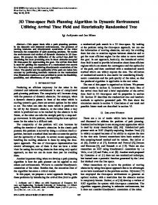
Move Robot Figure 4: The complete planning algorithm

The complete algorithm may be summarized by figure 4. The algorithm is an evolutionary approach, where a series of individuals representing solution are taken. As per our previous discussion, there are two different population maintained for the coarser and the final level. The

12

robot speed is fixed and within allowable time we need to optimize both these populations. Both finer and coarser optimizations are by separate EAs. The role of finer EA is to optimize the current path which would play a major role in deciding the immediate move of the robot. The coarser EA tries to optimize the global strategy being followed by the robot. In place of performing this step after a series of move of the robot, we prefer to perform this step at every robotic move to keep constant track of the changing environment. The algorithm stops once the robot reaches the final goal.

4. Results The proposed algorithm was implemented using a simulator made on a JAVA platform. The map was supplied as a JPEG image to this simulator. The map contained only the static obstacles. A separate program module parsed this image and converted it into a robotic map. The algorithm had separate modules for each of the two EAs discussed in the text. The robotic control and the control of the two EAs were done by a third module. Another module was used for specifying the behavior and movements of the dynamic obstacles. Finally a display module did the task of display of the robotic map and the movements of the robot and the obstacles. A number of executions were done with a variety of maps. These had both static and dynamic obstacles. In all these cases we saw that the robot was easily able to reach the goal position, starting from the specified goal position. The robot path was always optimal in nature. Further there was no visible collision of the robot in anywhere during its path. The first experiment was done with a variety of static obstacles. The complete setup of the algorithm was executed. The map was of size 1000 x 1000. The value of the map resolution reduction constant α was 20. The value of γ was 200. The master EA had the two mutation rates as 0.06 and 0.25. The maximum number of individuals could be 1000. At any generation, 68% individuals came from crossover, 15% from soft mutation, 5% from hard mutation, 2% from elite and 10% from the operator new. The slave EA was given similar parameters, except that the maximum number of individuals could be 100. The algorithm was executed for 100 generations at every step. The multi-objective parameters were fixed to 0.75 and 0.25 for both the evolutionary algorithms. The basic methodology of setting the parameters was that the algorithm execution time for every robotic step must be close to the speed of an average robot. The path traced by the robot is shown in figure 5. It can be easily seen that the robot was able to steer its way out of all the complex obstacles and reach the goal in an optimal path. This depicts the robot capability to solve complex maps. The second experiment was done using two static and two dynamic obstacles. The two static obstacles were circular in structure. The two dynamic obstacles were rectangular in structure and marched towards the goal as the robot made its move. The same set of parameters was used as stated in the previous experiment. The path traced by the robot is given in figure 6. The two solid rectangles denote the final positions of the dynamic obstacles and the empty rectangles show their initial positions. It can be easily seen that the robot could adjust its movements in such a manner so as to avoid collision with both these obstacles. In the entire path it did not have to wait for path clearance by the obstacles. It made moves such that it could easily cross the obstacles. This execution clearly denotes the capability of the robot to escape from static and dynamic obstacles and reach the goal in an optimal manner.

13

Figure 5: The execution of the algorithm in complex map

Figure 6: The execution of the algorithm with moving obstacles

Since we have used an evolutionary approach, one of the major factors to consider in this approach is to judge the algorithms capability to respond to sudden occurrence of obstacles. A robot moving might suddenly see some obstacle in front of it and would be expected to make its way out of it and reach the goal in an optimal manner. For this we give a simple map to the robot and allow it to move. However as soon as the robot is somewhere mid-way in its journey, we suddenly place an obstacle on its way. The robot is still able to steer out its way and reach the destination. The complete path traced by the robot is given in figure 7. This clearly shows that the robot is able to react to any sudden change in environment. In these experiments we have demonstrated the ability of the robot to solve complex maps, escape from static and dynamic obstacles, and to react to the sudden emergence of obstacles. Any

14

real life situation would primarily involve these conditions in different forms. Hence we may assume that the robot would be able to solve a variety of situations that it encounters in real life.

Figure 7: The execution of the algorithm with sudden obstacle emergence

An important characteristic of the algorithm is the role of parameters α and γ in its execution. The parameter α denotes the distribution between the coarser and finer hierarchies. A very large value of α would result in a very big map size of the finer hierarchy. This would necessitate the need of too much of computation time for the finer hierarchy to compute the optimal path. This would make the algorithm equivalent to a single EA. The entire path may hence be more optimal, but the dynamism would be gone. A very small value of this parameter would result in excessive size for the coarser hierarchy. The coarser hierarchy algorithm may now need a lot of computation time to give a guiding path for the finer hierarchy. This path would be next to the most optimal path that might not require further optimizations by the finer hierarchy. It may be easily observed that this behavior is also like the use of a single evolutionary approach. Accordingly the two parameters need to be set. The parameters however also have a dependence on the map. A reasonably simple map with few simple obstacles may be degraded to a good extent, without much loss of information. A large value of α is hence workable. This however would not be the case with a complex maps having too many complex obstacles in various parts. Keeping α large in such a case might show two unconnected regions of the map as connected, which would be wrong guidance to the finer hierarchy. The other factor γ denotes the vision of the finer hierarchy. A very large value might give a reasonably large part of the map to the finer hierarchy to work over. This would result in a very large computational time, but in return would lead to better results in terms of path optimality.

5. Conclusions In this paper we proposed a new algorithm for robotic path planning. The entire algorithm was broken into two stages of coarser and finer path planning. The coarser level used an evolutionary technique for path planning. This level worked only on a static map which had a reduced resolution. The path generated by this level of path planning was used for guiding the path

15

planning at the other level which was the finer level. This level of path planning was done on part of the actual high resolution map. The obstacles in this part were mobile which made the environment dynamic. For the planning purposes, this level extrapolated the motion of the various mobile obstacles. It assumed that the obstacles keep moving with the same speed and in the same direction. In this manner the robot is able to escape from the likely collisions with the mobile obstacles. The algorithm was tested against three types of scenarios. The first scenario was a complex static map. This had a variety of obstacles of different types of shapes and size. We observed that the robot could easily make its way out of all the obstacles. This depicted a high planning sense of the robot even in complex maps. This is an indication of the maze solving capability of the robot. This capability is of prime importance in robotics. The simple maps can be solved by almost any algorithm in literature. The real challenge in path planning is to solve the complex maps in computationally less time. The other experiment was done on the mobile obstacles. Two mobile obstacles were placed for the robot to make its way out. The robot in this case could easily escape out of all the static and dynamic obstacles and reach its way to the goal. This has a lot of relevance to the natural manner in which the humans walk and drive. We observe the manner in which the surrounding obstacles are moving and accordingly adjust our moves. The robot does the same thing in this movement strategy where it extrapolates the moves of the various obstacles so as to predict the future map and accordingly decide its moves. Based on experiments we observe that the robot was able to guess the future positions of the other obstacles. Accordingly it adjusted its move so as to escape from these obstacles. Any static path planning technique would have made the robot reach near the moving obstacle and then the robot would have to wait for the obstacle to cross, so as to continue its motion. The last experiment tested the ability of the robot to react to sudden emergence of obstacles. The evolutionary approaches normally take time for figuring out the optimal path and hence these are usually applied to the static environments only. The static environment path planning cannot cater to the needs of the dynamic environments and especially the sudden obstacle emergence where the map changes by a considerable amount at an instance of time. Our approach could however still make the robot escape from the obstacle and reach the goal safely. Both the hierarchies adjusted well to the sudden obstacle emergence. As a result as soon as the obstacle emerged, the robot changed its direction and moved at the near optimal path. The provision of addition of new individuals at both evolutionary algorithms was largely responsible for rapid generation of new individuals that could solve the problem. These paths may naturally not be optimized. However as the robot moves, the paths keep getting optimized. A few robotic moves give enough time for the algorithm to nicely optimize the paths. The algorithm made a variety of parameters for the generation of the path. In all the executions these parameters were kept as constant and generated fair enough paths whose optimality was visible. This makes it appear that the various parameters are passive in nature whose values may be fixed to some constant values. In reality all these parameters have a high degree of relevance to the map being used and the optimal values of the parameters would depend upon the map being used. This showcases the problem of optimal parameter setting of these parameters. The

16

problem is similar to the problem of parameter setting in the problems of machine learning, pattern recognition, or other neural and evolutionary approaches, where the parameters depend upon the data set, fitness landscape, etc. The optimal parameters can hence only be computed after analyzing the map and possibly running the algorithm a number of times. The parameter dependency motivates the engineering of self-adaptive systems for path planning that can adjust the various parameters on their own without any external or human input. A child or person walking does not need to set some parameters for making its way out. Similarly the robot needs to be fully autonomous without requiring any parameter setting for the path computation. The self-adaptive nature of the algorithm may be worked over into the future. Even though a lot of research in this domain may lead to good adaptation, we may not be able to build completely parameter less systems that are always optimal in their processing and output as per the No Free Lunch Theorems. The hierarchical solution to the problem of robotic path planning enabled its execution in the real-time mode with static and dynamic obstacles. Future research directions include mechanisms to strike a tradeoff between these two levels, dynamic control of the parameters of the two evolutionary algorithms as per the current convergence status and map, and inclusion of the non-holonomic constraints to ensure a smooth physical robotic movement by the robotic controller. The algorithm may further be analyzed to the behavior of the various parameters that play a big role in deciding path optimality and the tradeoffs with time. The time factor is highly dependent on the type of robot and its speed. The physical testing of the robot on a physical robot may further enable a clear understanding of the algorithm and parameter behavior.

6. References [1] Alvarez, Alberto, Caiti, Andrea & Onken, Reiner, “Evolutionary Path Planning for Autonomous Underwater Vehicles in a Variable Ocean”, IEEE Journal of Oceanic Engineering, Vol. 29, No. 2, April 2004, pp 418-429 [2] Carpin, Stefano & Pagello, Enrico, “An experimental study of distributed robot coordination”, Robotics and Autonomous Systems, Volume 57 , Issue 2, pp 129-133, February 2009 [3] Chen, Liang-Hsuan & Chiang, Cheng-Hsiung, “New Approach to Intelligent Control Systems With SelfExploring Process”, IEEE Transactions on Systems, Man and Cybernetics—Part B: Cybernetics, Vol. 33, No. 1, pp 56-66, February 2003 [4] Ge, Shuzhi Sam & Lewis, Frank L., “Autonomous Mobile Robot”, Taylor and Francis, 2006 [5] Hui, Nirman Baran & Pratihar, Dilip Kumar, “A comparative study on some navigation schemes of a real robot tackling moving obstacles”, Robotics and Computer-Integrated Manufacturing, (2009), doi:10.1016/j.rcim.2008.12.003 [6] Hwang, Joo Young; Kim, Jun Song; Lim, Sang Seok & Park, Kyu Ho, “A Fast Path Planning by Path Graph Optimization”, IEEE Transaction on Systems, Man, and Cybernetics—Part A: Systems and Humans, Vol. 33, No. 1, January 2003, pp 121-128 [7] Jolly, K.G.; Kumar, R. Sreerama & Vijayakumar, R., “A Bezier curve based path planning in a multi-agent robot soccer system without violating the acceleration limits”, Robotics and Autonomous Systems, Volume 57, Issue 1, 31 January 2009, pp 23-33 [8] Juidette, H. & Youlal, H., ” Fuzzy dynamic path planning using genetic algorithms”, IEEE Electronics Letters, 17th February 2000 Vol. 36 No. 4, pp 374-376 [9] Kala, Rahul, Shukla, Anupam & Tiwari, Ritu (2009a), Fusion of Evolutionary Algorithms and Multi-Neuron Heuristic Search for Robotic Path Planning, Proceedings of the IEEE 2009 World Congress on Nature & Biologically Inspired Computing (NABIC '09), pp 684 - 689, Coimbatote, India [10] Kala, Rahul, Shukla, Anupam & Tiwari, Ritu (2009b), Robotic Path Planning using Multi Neuron Heuristic Search, Proceedings of the ACM 2009 International Conference on Computer Sciences and Convergence Information Technology (ICCIT 2009), pp 1318-1323, Seoul, Korea

17 [11] Kala, Rahul; et al. (2009c) “Mobile Robot Navigation Control in Moving Obstacle Environment using Genetic Algorithm, Artificial Neural Networks and A* Algorithm”, Proceedings of the IEEE World Congress on Computer Science and Information Engineering (CSIE 2009), ieeexplore, April 2009, Los Angeles/Anaheim, USA [12] Kala, Rahul, Shukla, Anupam, Tiwari, Ritu, “Fusion of Probabilistic A* Algorithm and Fuzzy Inference System for Robotic Path Planning”, Artificial Intelligence Review, Springer, doi.: [13] Kambhampati, Subbarao & Davis, Larry S., “Multiresolution Path Planning for Mobile Robots”, IEEE Journal of Robotics and Automation, Vol RA-2, No. 3, September 1986, pp135-145 [14] Lai, Xue-Cheng; Ge, Shuzhi Sam & Mamun, Abdullah Al, “Hierarchical Incremental Path Planning and Situation-Dependent Optimized Dynamic Motion Planning Considering Accelerations”, IEEE Transactions on Systems, Man, and Cybernetics—Part B: Cybernetics, Vol. 37, No. 6, December 2007, pp 1541-1554 [15] Lin, Hoi-Shan; Xiao, Jing & Michalewicz, Zbigniew, “Evolutionary Algorithm for Path Planning in Mobile Robot Environment”, Proceedings of the First IEEE Conference on Evolutionary Computation (ICEC'94), pp 211216, Piscataway, New Jersey, June 1994. Orlando, Florida [16] O’Hara, Keith J.; Walker, Daniel B. & Balch, Tucker R., “Physical Path Planning Using a Pervasive Embedded Network”, IEEE Transactions on Robotics, Vol. 24, No. 3, June 2008, pp 741-746 [17] Peasgood, Mike; Clark, Christopher Michael & McPhee, John, “A Complete and Scalable Strategy for Coordinating Multiple Robots Within Roadmaps”, IEEE Transactions on Robotics, Vol. 24, No. 2, April 2008. pp 283-292 [18] Pozna, Claudiu, et. al., “On the design of an obstacle avoiding trajectory: Method and simulation”, Mathematics and Computers in Simulation, (2009), doi:10.1016/j.matcom.2008.12.015 [19] Shibata, Takanori; Fukuda, Toshio & Tanie, Kazuo, “Fuzzy Critic for Robotic Motion Planning by Genetic Algorithm in Hierarchical Intelligent Control”, Proceedings of 1993 International Joint Conference on Neural Networks, pp 77-773 [20] Shukla, Anupam & Kala, Rahul; “Multi Neuron Heuristic Search”, International Journal of Computer Science and Network Security, Vol. 8, No. 6, pp 344-350, June 2008 [21] Shukla, Anupam; Tiwari, Ritu & Kala, Rahul; “Mobile Robot Navigation Control in Moving Obstacle Environment using A* Algorithm”, Intelligent Systems Engineering Systems through Artificial Neural Networks, ASME Publications, Vol. 18, pp 113-120, Nov 2008 [22] Shukla, Anupam, Tiwari, Ritu, Kala, Rahul (2009), Mobile Robot Navigation Control in Moving Obstacle Environment using Genetic Algorithms and Artificial Neural Networks, International Journal of Artificial Intelligence and Computational Research, Vol. 1, No. 1, pp 1-12, June 2009 [23] Shukla, Anupam, Tiwari, Ritu, Kala, Rahul (2010), Real Life Applications of Soft Computing, CRC Press [24] Tsai, Chi-Hao; Lee, Jou-Sin & Chuang, Jen-Hui, “Path Planning of 3-D Objects Using a New Workspace Model”, IEEE Transactions on Systems, Man, and Cybernetics—Part C: Applications and Reviews, Vol. 31, No. 3, August 2001, pp 405-410 [25] Urdiales, C.; Bantlera, A.; Arrebola, F. & Sandova1, F., “Multi-level path planning algorithm for autonomous robots”, IEEE Electronic Letters, 22nd January 1998, Vol. 34 No. 2, pp 223-224 [26] Xiao, Jing; Michalewicz, Zbigniew; Zhang, Lixin & Trojanowski, Krzysztof, “Adaptive Evolutionary Planner/Navigator for Mobile Robots”, IEEE Transactions on Evolutionary Computation, Vol. 1, No. 1, April 1997, pp 18-28 [27] Zhu, David & Latombe, Jean-Claude, “New Heuristic Algorithms for Efficient Hierarchical Path Planning”, IEEE Transactions on Robotics and Automation, Vol. 7, No. 1, February 1991, pp 9-20