Dynamic Modeling of Internet Traffic for Intrusion Detection E. Jonckheere, K. Shah and S. Bohacek University of Southern California, Los Angeles, CA- 90089-2563.
[email protected] Abstract Computer network traffic is analyzed via state space models and statistical techniques such as linear and nonlinear canonical correlation analyses and mutual information. As an application, the models and the statistical techniques are utilized to detect UDP flooding attacks. This work indicates that mutual information is a powerful tool for the detection of such attacks. Our approach is topology independent and our findings are tested on the so-called dumbbell and parking-lot topologies. This research was supported by DARPA Contract N66001-00-C-8044.
length, ...) are candidates for dynamical modeling, but here we shall focus on link utilization. No distinction between control and data packets is made at this stage. The signals are themselves generated by ns, the network simulator. Two different network topologies have been retained–the “dumbbell” topology and the “parking lot” topology. In both the cases, the link utilization is observed at a router. The link utilization is integrated over a sampling period ranging from 0.1 to 20 sec. Our study is somehow 4-fold: dumbbell versus parking lot topology, linear versus nonlinear, for varying sampling periods, and for varying “lags,” where the lag is defined as the length of the data record utilized in the CCA.
2 Simulation Setup 1 Introduction Traffic signal analysis has seen renewed interest over the past few years and has so far for the most part focused on modeling such phenomena as self-similarity and burstyness, building on the theory of α-stable distributions with infinite variances [1], [2]. Here, we rather focus on the dynamical aspects of the modeling, yet keeping in mind that the traffic signals inevitably contain a certain degree of randomness due to the fact that the traffic sources appear unpredictable from the observation point, typically a router. A modeling tool that fairly naturally applies in this context is the Canonical Correlation Analysis (CCA) between the past and the future of the process. The motivation for a dynamic modeling of the signals is that, if a baseline (FTP, HTTP,...) traffic model has been identified, if the model is subsequently confronted with traffic data, and if at a certain point in time the model no longer fits the data, some suspicious activity must be on going. CCA also yields as a by-product the Akaike mutual information between the past and the future, which provides a statistical signature of the signal. The latter ineluctably changes under attack and hence produces yet another intrusion detection scheme. Several signals (link utilization, packet arrival, queue
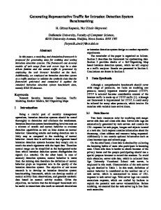
We used the Network Simulator (ns)developed by LBNL to set up our simulation environment [3]. Ns is a discrete event simulator widely accepted for networking research. It provides a substantial support for simulation of TCP, routing, and multicast protocols over wired and wireless (local and satellite) networks. Moreover, ns generates Constant Bit Rate (CBR) traffic, TELNET, FTP, HTTP, etc. The simulator also has a small collection of mathematical functions that can be used to implement random variate generation (exponential, uniform, Pareto, etc.) We used this capability to setup the network environment that synthesized HTTP, FTP, and CBR traffic. We performed our tests on two different topologies. The first topology under consideration was the “Dumbbell” topology (Fig. 1). We set the nodes Si ( i = 1,2,...,5) as sources and the nodes Di (i=1,2,...,5) as destinations. Normal traffic was generated by sending a mixture of HTTP and FTP traffic from the sources (Si ) to the corresponding destinations (Di ) at random times. For HTTP traffic, the file size distribution was modeled as a general ON/OFF behavior with a combination of heavy-tailed and light tailed sojourn times, while the interpage time and the interobject per page time distributions were set to be exponential. The page
SD1 1
SC11
0 D2
S2
S
1
D
S3
N1
D3
N2
S
2
D
D4
S4
CSn 5
D S
3
1 0
D
of HTTP and FTP traffic, while UDP pakcet storm attack is simulated by sending CBR traffic from the sources S1, S2, S3 to the destination S4.
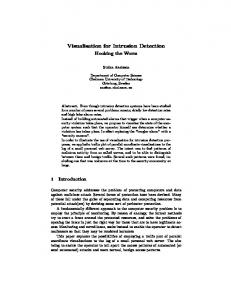
2
4
Sm5 D
Figure 1: Dumbbell topology. Normal traffic is a mix
1
3
1 0
1 1
Figure 2: Parking lot topology. Baseline traffic is a mix of HTTP and FTP traffic, while UDP flooding attack is simulated by sending CBR traffic from node 3 to node 4.
3 Canonical Correlation Analysis size was set to be constant and the object per page size to be Pareto to replicate today’s network bursty traffic [4], [2]. For FTP traffic, files of random sizes were sent at random times [5]. We monitored the traffic flowing from N1 to N2 , the bottleneck, or “choke point,” link. To simulate a UDP packet storm attack [6], a large number of small size Constant Bit Rate (CBR) packets were sent over some UDP connections from the sources S1 , S2 , S3 to the victim destination D4 on the top of the normal traffic. Each trial was executed for 30000 simulated seconds, logging the traffic at the 0.01 second granularity. For a particular scenario, the bottleneck link was 1.5 Mbps and the non-bottleneck links were 10 Mbps and the latency of the each link was set to 20 ms. UDP flooding attack was generated by each source having 5 UDP agents sending CBR packets of the size 200 bytes at the rate of 0.005 second/bytes to the victim. In the more complicated “Parking Lot” topology (Fig. 2), we set the nodes Si ( i = 1,2,...,10) as sources and the nodes Di (i = 1,2,...,10) as destinations. A dynamical model for normal TCP traffic was synthesized from the signals obtained by sending a mixture of FTP and HTTP traffic from the sources to their downstream destinations at random times. The normal traffic was monitored along the path from node 3 to node 4. In addition to this background traffic (HTTP and FTP), a large number of small size CBR packets were sent over some UDP connections from source node 3 to the victim node 4 to model the attack scenario. We monitored the link utilization along the same path, from node 3 to the node 4, and gathered the simulated attack data. Simulation results were obtained for several trials of ns. Each run was executed for 30000 simulated seconds, logging the traffic at the 0.01 second granularity. For a particular case, link speed was 10 Mbps and the latency of the each link was set to 20 ms. UDP packet storm was generated by 15 UDP agents sending CBR packets of a size of 200 bytes at a rate of 0.005 second/bytes to the victim.
CCA is a second moment technique. In its linear version, it relies on the second moments of the process itself, and as such the analysis cannot be carried out on those self-similar traffic signal models with infinite variance [1]. One should keep in mind, however, that infinite variance processes are a convenient way of modeling exactly self-similar processes and that in practice self-similarity is observed only over finitely many scales. Other considerations that support the finite variance hypothesis include the small size of the network on which the traffic is simulated and the finite bandwidth of the links. These observations corroborate recent work at AT&T [7], which calls into question whether real traffic is self-similar. In the nonlinear CCA, these issues become irrelevant, because the variance analysis is applied to a nonlinear distortion of the original process, which is restricted to result in a finite variance process. 3.1 Linear state space models Here {y(k) ∈ [−b, +b] : k = ..., −1, 0, +1, ...} is the centered link utilization signal, bounded by the bandwidth, viewed as weakly stationary process with finite covariance E(y(i)y(j)) = Λi−j defined over the probability space (Ω, A, µ). The past and the future of the process are defined, respectively, as y− (k) = (y(k), y(k − 1), ..., y(k − L + 1))T , y+ (k) = (y(k + 1), ..., y(k + L))T
where L is the lag. The ability to devise a good model can be gauged from the Kolmogorov-Sinai, or Shannon, mutual information between the past and the future [8],[9],[10], I(y− , y+ ) = h(y+ ) − h(y+ |y− ) Z Z p (y− , y+ ) p (y− , y+ ) dy− dy+ = log p (y− ) p (y+ ) In the above, h(y+ ) is the Shannon entropy of the future and h(y+ |y− ) is the conditional entropy of the fu-
ture given the past. To proceed from a numerical algebra point of view, the covariances of the past and the future are factored as T (k)) = L− LT− , E(y− (k)y−
T E(y+ (k)y+ (k)) = L+ LT+
and the canonical correlation is defined and Singular Value Decomposed (SVDed) as ¡ ¢ −T T T Γ (y− , y+ ) = L−1 − E y− (k)y+ (k) L+ = U ΣV where U, V are orthogonal matrices and 0 σ1 . . . .. , 1 > σ > . . . > σ > 0 .. Σ = ... 1 L . . 0
···
It is a bit tedious to show (although it is implicitly contained in Akaike [11]) that the residual noise w(k) is white and furthermore Q = E(w(k)wT (k)) = Σ21 − AΣ21 AT Next, a regression of y(k + 1) on x(k) is done, yielding the matrix C as ¢¡ ¢−1 ¡ C = E y(k + 1)xT (k) E(x(k)xT (k) T −1 = (Λ1 , Λ2 , ..., ΛL ) L−T − U1 Σ1
Again, the residual error v(k) can be shown to be white and R = E(v(k)v(k)) = Λ0 − CΣ21 C T
σL
The σ’s are called canonical correlation coefficients (CCC’s). If the process is Gaussian, it is well known that ∆(y− , y+ ) = I(y− , y+ ) where, ¡ ¢ 1 ∆(y− , y+ ) : = − log det I − ΓT (y− , y+ ) Γ (y− , y+ ) 2
At this stage, it is customary to assume that there are only a restricted number D ≤ L of significant CCC’s, which we group in Σ1 , and we further partition Σ and the orthogonal matrices conformably as µ ¶ µ ¶ ¶ µ U1 Σ1 0 V1 U= , Σ= , V = U2 V2 0 0 The canonical past and the canonical future [11] are defined as y− (k) = U1 L−1 − y− (k),
y+ (k) = V1 L−1 + y+ (k)
The state is defined as the minimum collection of pastmeasurable random variables necessary to predict the future, that is, E(y+ (k) |y− (k)). A basis of such collection of random variables is given by ´ ³ x(k) = E y+ (k)|y− (k) = Σ1 y− (k)
The state transition matrix A is defined as the least squares fit regression matrix of x(k + 1) on x(k), viz., ¢¡ ¢−1 ¡ A = E x(k + 1)xT (k) Ex(k)xT (k) − → −T T −1 = Σ1 U1 L−1 − Λ L− U1 Σ1 − → where Λ denotes Λ shifted to the right by one position, that is, Λ1 Λ2 ··· ΛL Λ1 · · · ΛL−1 − → Λ0 Λ = . . .. .. .. .. . . Λ1 ΛL−2 ΛL−3 · · ·
Finally, it is also readily found that (2) S = E(w(k)v(k)) = Σ1 U1 L−1 − AΣ21 C T − Λ
− → Where, Λ(2) is the 2nd row of Λ . Hence, we have a state space model of the form [12] x(k + 1) = Ax(k) + w(k) y(k + 1) = Cx(k) + v(k) In order to confront the data with the model, we need to know the state x(k), which could be computed as Σ1 y− (k). It is, however, more efficient to get an estimate of the state provided by the Kalman filter x b(k + 1|k + 1) = Ab x(k|k) + K(y(k + 1) − Cb x(k|k)) y(k + 1) = C x b(k|k) + (y(k + 1) − Cb x(k|k))
Since y(k + 1) − Cb x(k|k) is well known to be a white noise, called innovation, the Kalman filter provides yet another state space model, referred to as innovation representation [13]. The Kalman gain is given by ¢−1 T ¡ (B P AT + S) K = − R + CP C T
and P = E(x(k) − x b(k|k))(x(k) − x b(k|k))T is the stabilizing solution to the discrete-time algebraic Riccati equation P
= AP AT + Q
¢−1 T ¡ (B P AT + S) −(AP B + S T ) R + CP C T
A few numerical remarks: It is customary to define L± to be lower triangular (Cholesky factorization), although L± could be defined upper triangular (“anti-Cholesky” factorization), in which case Γ is near-Hankel and in fact will be Hankel for L = ∞. The particular factorization does not affect the CCC’s. T (k)) might be marginally positive definite, E(y± (k)y± resulting in problems in the Cholesky factorization; there is thus a need to monitor the condition number T (k)). of E(y± (k)y±
3.2 Nonlinear state space models Here, we allow the zero-mean process {y(k) ∈ < : k = ..., −1, 0, +1, ...} to be of infinite variance (for example, an α-stable, H-self-similar process [1]). The nonlinear CCA [8],[9] is an attempt to reach the mutual information, in the nongaussian setup, as sup (∆(f(y− ), g(y+ ))) ≤ I(y− , y+ ) f,g
where f, g :