Dynamic Output Feedback Compensation Control for Discrete Closed

Hindawi Mathematical Problems in Engineering Volume 2017, Article ID 6427807, 11 pages https://doi.org/10.1155/2017/6427807

Research Article Dynamic Output Feedback Compensation Control for Discrete Closed-Loop Nonlinear System with Multiple Time-Delays Wei Zheng,1 Hong-bin Wang,1,2 and Zhi-ming Zhang3 1

Institute of Electrical Engineering, Yanshan University, Qinhuangdao 066004, China Liren Institute, Yanshan University, Qinhuangdao 066000, China 3 China National Heavy Machinery Research Institute, Xi’an 710000, China 2

Correspondence should be addressed to Wei Zheng; [email protected] Received 27 March 2017; Revised 13 June 2017; Accepted 2 July 2017; Published 9 August 2017 Academic Editor: Asier Ibeas Copyright © 2017 Wei Zheng et al. This is an open access article distributed under the Creative Commons Attribution License, which permits unrestricted use, distribution, and reproduction in any medium, provided the original work is properly cited. This paper addresses the dynamic output feedback control problem for a class of discrete system with uncertainties and multiple time-delays. First, the system is decomposed into two subsystems based on the output matrix and input control matrix. Secondly, a dynamic compensator is employed for the first subsystem, and then, given the multiple uncertainties, the output feedback controller is designed based on the second subsystem and the dynamic compensator. Thirdly, by choosing the Lyapunov-Krasovskii function, it can be seen that the developed controller makes the closed-loop system convergent to an adjustable region, which can be rendered arbitrary small by adjusting design parameters. Compared with the previous researches, the proposed controller is not only smooth and memoryless, but also only dependent on the system output. Furthermore, with the given dynamic compensator, the controller design conditions are relaxed, while the approach is extended to the conventional nonlinear system. Finally, numerical example is given to illustrate the effectiveness of the theoretical results.

1. Introduction Many practical systems are the large nonlinear systems and consist of time-delays in the real world, such as various engineering systems, digital communication systems, urban traffic networks, and economic systems. Stability analysis for time-delay dynamic systems has been one of the focused study topics in the past decades, and many accomplishments have been made; see [1–5]. Many researches often used the Razuminkin lemma and Lyapunov functional methods for the design and analysis of time-delay systems. For a practical system, it may be a difficult mission to obtain all the state variables; thus the output feedback control approach is proposed. Compared with the state feedback control, the output feedback control problem is more challenging because of the limited information of state variables. It is well known that dynamic output feedback and static output feedback received lots of attention in various engineering systems. Compared with the previous state feedback control, the output feedback control issues are more challenging because the state variables information is limited.

Li and Jia [6] considered the nonfragile dynamic output feedback control for linear systems with time-varying delay. Lv et al. [7] proposed the adaptive output feedback consensus protocol design for linear systems with directed graphs. Wei et al. [8] proposed the robust and reliable 𝐻-∞ static output feedback (SOF) control for nonlinear systems with actuator faults in a descriptor system framework. In [9, 10], the dynamic output feedback control issue and the static output feedback control issue for the linear systems were discussed; the new model and system order were presented. For the unknown nonlinear system, robust adaptive output feedback control strategy was proposed for dealing with the nonlinear uncertain issues [11]. Zhu et al. [12] considered the adaptive output feedback control issue for an uncertain linear time-delay system. Zhou [13] investigated the observerbased output feedback control problem for discrete-time linear systems with time-delays. Qiu et al. [14] considered the static output feedback 𝐻-∞ control issue for continuous time systems, and a new Lyapunov functions was proposed. In the above researches, the time-delay systems are all considered as the linear form. For the nonlinear uncertain systems with

2 time-delays, a lot of investigations have been done. In [15], a network-based feedback control for time-delay systems was developed, which is based on the quantization and dropout compensation. Yao et al. [16] investigated the extendedstate-observer-based output feedback control for hydraulic systems by employing the back-stepping control technique. Xia et al. [17] designed the smooth speed controller for lowspeed high-torque permanent-magnet synchronous motor. Chen [18] considered the active magnetic bearing system and designed the delay dependent nonlinear smooth output feedback control. Aiming at the output feedback control issues, in [19], the dynamic robust fault tolerant tracking controller was investigated to estimate the unknown inputs models and unmeasurable system state variables. In [20], Toscano and Lyonnet designed the delay-independent static robust output feedback controller. Then Xian et al. [21] constructed the discontinuous output feedback controller and velocity observer for nonlinear mechanical systems. By investigating the nonlinear robust control systems, Chae and Nguang [22] and Wei et al. [23] proposed the robust 𝐻∞ dynamic output feedback control method for solving the tracking control problem. In [24], a novel smooth output feedback controller was constructed for continuous systems with time-delays by Hua and Guan. It is well known that static output feedback is frequently encountered in practical control systems, but some strict design conditions should be considered in the system. However, all the above design technique has to predetermine the feedback gains before checking the stability conditions of the closed-loop system. In various engineering systems, all of the state variables are not available. Thus, it is necessary to design dynamic output feedback controller. The dynamic output feedback technique is more flexible and the required conditions on the considered systems are less conservative. Furthermore, the previous many methods are efficient for the control design of the time-delays system, but the system controller is not continuous and the accuracy time-delays are often needed for achieving the control objectives. The topic of this study can be viewed as the discrete counterpart of the topic in [19], in which the output control issue for continuous time system with time-delays was studied. Based on the above contents, we consider the dynamic output feedback control issues for a nonlinear discrete multiple time-delays system and aim to construct the smooth and memoryless output feedback controller. In this paper, we study the issues of smooth dynamic output feedback control of discrete-time multiple time-delays system. The parametric uncertainties are assumed to be a linear fractional form which can include the norm bounded uncertainty as its special case. For the closed-loop system, a dynamic compensation controller is designed to reduce the control design requirement. And then the output feedback controller with adaptive law is constructed based on the compensation control. With the help of the proposed Lyapunov functional, the stability of the whole system is well proved. Furthermore, we have extended the results to the general nonlinear case and discussed the dynamic output feedback control issue accordingly. Finally, numerical simulations are performed to show the potential of the proposed strategy.

Mathematical Problems in Engineering

2. System Description The dynamic model in this section is characterized by discrete-time and multiple time-delays, whose relationship exhibits the uncertain characteristics to the nonlinear practical systems. Many practical systems are the large nonlinear systems and consist of multiple time-delays in the real world, such as various engineering systems and digital communication systems. Thus, let us consider a nonlinear discrete-time system with multiple time-delays as follows: 𝑟

𝑥 (𝑘 + 1) = ∑𝐴 𝑗 𝑥 (𝑘 − 𝜏𝑗 ) + 𝐵 (𝑢 (𝑘) 𝑗=0

+ 𝑓 (𝑥 (𝑘) , 𝑥 (𝑘 − 𝜏1 ) , 𝑥 (𝑘 − 𝜏2 ) , . . . , 𝑥 (𝑘 − 𝜏𝑟 ))) ,

(1)

𝑦 (𝑘) = 𝐶𝑥 (𝑘) , where 𝑥(𝑘) ∈ 𝑅𝑛 is the state variable, 𝑢(𝑘) ∈ 𝑅𝑚 and 𝑦(𝑘) ∈ 𝑅𝑝 are the control input and output of the system (1), respectively, 𝐴 𝑗 ∈ 𝑅𝑛×𝑛 , 𝐵 ∈ 𝑅𝑛×𝑚 , and 𝐶 ∈ 𝑅𝑝×𝑛 are the state matrix, input matrix, and output matrix, respectively, and all matrices are constant matrices with appropriate dimensions. We assume 𝑛 ≥ 𝑝 > 𝑚 with the following condition: rank(CB) = 𝑚 ⋅ 𝜏𝑗 is the multiple time-delays that satisfies 𝜏𝑗 (𝑘 + 1) ≤ 𝜏𝑗∗ , 𝜏𝑗 ≤ 𝜏𝑗 for 𝑗 = (0, 2, . . . , 𝑟), and 𝜏0 = 0, where 𝜏𝑗∗ and 𝜏𝑗 are positive scalars. The nonlinear function𝑓(⋅) is uncertain and contains multiple time-delays state with 𝑓(0, 0, . . . , 0) = 0. For the nonlinear uncertain vector function 𝑓(⋅) of the system (1), there exist the following assumptions. Assumption 1. The nonlinear function vector 𝑓 satisfies 𝑟

󵄩 󵄩 ∑ 𝜗𝑗𝑇 𝛼𝑗 (󵄩󵄩󵄩󵄩𝑥 (𝑘 − 𝜏𝑗 )󵄩󵄩󵄩󵄩)

𝑗=0

(2)

󵄩 󵄩 ≥ 󵄩󵄩󵄩𝑓 (𝑥 (𝑘) , 𝑥 (𝑘 − 𝜏1 ) , 𝑥 (𝑘 − 𝜏2 ) , . . . , 𝑥 (𝑘 − 𝜏𝑟 ))󵄩󵄩󵄩 , where 𝜗𝑗 ∈ 𝑅𝑝𝑗 is unknown constant vector and 𝛼𝑗 (⋅) = [𝛼𝑗1 (⋅), 𝛼𝑗2 (⋅), . . . , 𝛼𝑗𝑖 (⋅)]𝑇 with 𝛼𝑗𝑖 (⋅) is a known increasing function and 𝛼𝑗𝑖 (0) = 0. And there exist nonlinear functions 𝛼𝑗𝑖 (⋅) such that 𝑥𝛼𝑗𝑖 (𝑥) ≥ 𝛼𝑗𝑖 (𝑥) for all 𝑗 and 𝑖. Remark 2. System (1) contains the functions with multiple time-delays and nonlinear uncertain. The sliding mode state feedback control scheme was presented in [25] and the stability was proven. For system (1), the full-order observer was designed and then the observer-based sliding mode feedback controller was designed by Chen and Fu [26]. It is generally known that some strict conditions on the control system will be imposed by the static output feedback control. Furthermore, the adaptive sliding-mode control method needs the accurate time-delays value of system state for control implementation. The static output feedback sliding-mode control scheme was discussed in [27]. In this study, the objective is to design a smooth dynamic output feedback controller for system (1) with Assumption 1 such that the designed controller makes the solutions of the system exponentially convergent to a ball.


3

Remark 3. With the parameters unknown, the adaptive strategy was presented to estimate the parameters of system or uncertain bound parameters. In [7], the adaptive output feedback control problem was discussed with some unknown interconnections. With these researches containing the nonlinear function in the system, it can be seen that the schemes are not enforceable to system (1). For the problem formulated, there are three challenging problems as follows: how to design a dynamic compensator with the output feedback signal; how to reduce the influence of uncertain parameters; and how to design the output feedback controller for the time-delays system. Our control objective is to solve the above three issues, and then the controller will be easy to implement in practical systems. With the above contents, we assume that 𝐵 = 𝑇 𝑇 [0(𝑛−𝑚)×𝑚 𝐵𝑚×𝑚 ] , 𝐶 = [0(𝑛−𝑝)×𝑝 𝐷𝑝×𝑝 ] , where 𝐵𝑚×𝑚 and 𝐷 satisfy the following conditions: rank(𝐵𝑚×𝑚 ) = 𝑚 and

where 𝐴𝑗11 = 𝐴 𝑗11 , 𝐴𝑗12 = 𝐴 𝑗12 𝐸−1 , 𝐴𝑗21 = 𝐸𝐴 𝑗21 , 𝐴𝑗22 = 𝐸𝐴 𝑗22 𝐸−1 . Since matrices 𝐸 and 𝐵 are nonsingular, there exist 𝐸𝐵 which is also nonsingular. In the next section, we will consider the controller design problem for system (4).

3. Controller Design 3.1. Design the Dynamic Compensator. For subsystem-𝑥1 of system (4), an augmented dynamic system is designed by the following form: 𝑦2 (𝑘) = 𝐶𝑙 𝜁 (𝑘) + 𝐷𝑙 𝑦1 (𝑘) , 𝜁 (𝑘 + 1) = 𝐴 𝑙 𝜁 (𝑘) + 𝐵𝑙 𝑦1 (𝑘) ,

where 𝜁 ∈ 𝑅𝑛−𝑚 , 𝑦2 ∈ 𝑅𝑚 , 𝐴 𝑙 , 𝐵𝑙 , 𝐶𝑙 , and 𝐷𝑙 are designed with appropriate dimensions. With (4) and (5), one has

𝑥𝑇

𝐷𝐷𝑇 = 𝐷𝑇 𝐷 = 𝑈𝑚 , 𝑈𝑚 is the identity matrix. Let 𝑥 = [ 𝑥1𝑇 ]

𝑟

𝛿 (𝑘 + 1) = ∑ 𝑁𝑗 𝛿 (𝑘 − 𝜏𝑗 ) + 𝐼𝛿 (𝑘) + 𝑤,

2

with 𝑥1 ∈ 𝑅𝑛−𝑚 and 𝑥2 ∈ 𝑅𝑚 ; then system (1) can be rewritten as follows: 𝑟

𝑥1 (𝑘 + 1) = ∑ (𝐴 𝑗12 𝑥2 (𝑘 − 𝜏𝑗 ) + 𝐴 𝑗11 𝑥1 (𝑘 − 𝜏𝑗 )) ,

𝑗=1

𝑧 (𝑘) = 𝑦2 (𝑘) − 𝑦2 (𝑘) ,

𝑟

𝑥1 (𝑘) 𝛿 (𝑘) = [ ], 𝜁 (𝑘)

𝑦2 (𝑘 + 1) = ∑ (𝐴 𝑗22 𝑥2 (𝑘 − 𝜏𝑗 ) + 𝐴 𝑗21 𝑥1 (𝑘 − 𝜏𝑗 )) 𝑗=0

(3)

̃ 𝐴012 𝐶𝑙 𝐴011 + 𝐴012 𝐷𝑙 𝐶 𝐼=[ ], ̃ 𝐴𝑙 𝐵𝑙 𝐶

+ 𝐵𝑢 (𝑘) ,

where 𝐴 𝑗11 , A𝑗12 , 𝐴 𝑗21 , 𝐴 𝑗22 are the decomposition matrix of 𝑦𝑇

𝐴 𝑗 . With 𝑚 < 𝑝, one has 𝑦 = [ 𝑦1𝑇 ], where 𝑦1 ∈ 𝑅𝑝−𝑚 and 2

𝑦2 ∈ 𝑅𝑚 . Consider the structures of matrices 𝐵 and 𝐶; there ̃ ∈ 𝑅(𝑝−𝑚)(𝑛−𝑚) exist the nonsingular matrices 𝐸 ∈ 𝑅𝑚×𝑚 and 𝐶 ̃ 1 and 𝑦2 = 𝐸𝑥2 . such that 𝑦1 = 𝐶𝑥 With the above analysis, system (1) is further rewritten as follows: 𝑟

In addition, for (6), choose the following discrete LyapunovKrasovskii function: 𝑟

𝑉1 = ∑ ∫

𝑗=0

𝑗=1 𝑘−𝜏𝑗 𝑟

+∑∫

𝑇

𝑇

],

[ (𝐸𝑥2 ) ]

0

𝑘

∫

𝑘+𝜗

(8) 𝑐(𝜎−𝑘) 𝑇 ̇

𝑒

𝛿 (𝜎) 𝑍𝑗 𝛿̇ (𝜎) 𝑑𝜎 𝑑𝜗,

𝑟

Δ𝑉1 ≤ ∑ (𝜏𝑗 𝛿𝑇 (𝑘 + 1) 𝑍𝑗 𝛿 (𝑘 + 1)

𝑗=0

+ 𝐸𝐵𝑢 (𝑘) ,

𝑒𝑐(𝜎−𝑘) 𝛿𝑇 (𝜎) 𝑅𝑗 𝛿 (𝜎) 𝑑𝜎 + 𝛿𝑇 (𝑘) 𝑃𝛿 (𝑘)

𝑗=1 −𝜏𝑗

𝑟

𝑦2 (𝑘 + 1) = ∑ (𝐴𝑗21 𝑥1 (𝑘 − 𝜏𝑗 ) + 𝐴𝑗22 𝑦2 (𝑘 − 𝜏𝑗 )) + 𝐸𝐵𝑓 (𝑥 (𝑘) , 𝑥 (𝑘 − 𝜏1 ) , . . . , 𝑥 (𝑘 − 𝜏𝑟 ))

𝑘

where 𝑃, 𝑅𝑗 , 𝑍𝑗 are positive matrices and 𝑐 and 𝜎 are positive scalars. Now, taking the forward difference of (8), the following inequality holds:

𝑥1 (𝑘 + 1) = ∑ (𝐴𝑗11 𝑥1 (𝑘 − 𝜏𝑗 ) + 𝐴𝑗12 𝑦2 (𝑘 − 𝜏𝑗 )) ,

̃ 1) (𝐶𝑥

(7)

̃ 𝐴𝑗12 𝐶𝑙 𝐴𝑗11 + 𝐴𝑗12 𝐷𝑙 𝐶 𝑁𝑗 = [ ]. 0 0

𝑥1𝑇 𝑦 (𝑘) = 𝐶 [ 𝑇 ] , 𝑥2

𝑦 (𝑘) = [

(6)

where 𝑤 = ∑𝑟𝑗=0 𝐴𝑗12 𝑧(𝑘 − 𝜏𝑗 ) in which

𝑗=0

+ 𝐵𝑓 (𝑥 (𝑘) , 𝑥 (𝑘 − 𝜏1 ) , . . . , 𝑥 (𝑘 − 𝜏𝑟 ))

(5)

𝑗=1

(4) −∫

𝑘

𝑘−𝜏𝑗

𝑟

𝑒−𝑐𝜏𝑗 𝛿𝑇̇ (𝜎) 𝑍𝑗 𝛿̇ (𝜎) 𝑑𝜎) + ∑ (𝛿𝑇 (𝑘) 𝑅𝑗 (𝑘) 𝑗=1

− (1 − 𝜏𝑗∗ ) 𝑒−𝑐𝜏𝑗 𝛿𝑇 (𝑘 − 𝜏𝑗 ) 𝑅𝑗 𝛿 (𝑘 − 𝜏𝑗 )) + 2𝛿𝑇 (𝑘) ⋅ 𝑃𝛿 (𝑘 + 1) − 𝑐𝑉1 + 𝑐𝛿𝑇 (𝑘) 𝑃𝛿 (𝑘) .

(9)

4

Mathematical Problems in Engineering with 𝐺 < 0 and 𝐹𝑖 < 0 in Theorem 4; the following inequalities hold:

Note that 𝑟

𝑟

𝑖=1

𝑗=0

2∑ ( ∑ 𝛿𝑇 (𝑘 − 𝜏𝑗 ) 𝑇𝑖𝑗 + 𝑤𝑇 (𝑘) 𝑇𝑖(𝑟+1) )

𝑎𝑇 𝐺𝑎 ≤ 0, (10)

× (𝛿 (𝑘) − ∫

𝑘

𝑘−𝜏𝑗

𝑥𝑇 (𝑘, 𝜁) 𝐹𝑖 𝑥 (𝑘, 𝜁) ≤ 0,

𝛿̇ (𝜎) 𝑑𝜎 − 𝛿 (𝑘 − 𝜏𝑖 )) = 0,

𝑟

∑∫

𝑖=1 𝑘−𝜏𝑗

where 𝑇𝑖𝑗 is weight matrix. Consider (6), (9), and (10); we have

+ ∑∫

𝑘


𝑇

𝑥 (𝑘, 𝜁) 𝐹𝑖 𝑥 (𝑘, 𝜁) 𝑑𝜁,

(15)

𝑥𝑇 (𝑘, 𝜁) 𝐹𝑖 𝑥 (𝑘, 𝜁) 𝑑𝜁 ≤ 0;

one has

Δ𝑉1 ≤ 𝜀 ‖𝑤‖2 − 𝑐𝑉1 + 𝑎𝑇 𝐺𝑎 𝑟

𝑘

𝑟

𝑎𝑇 𝐺𝑎 + ∑ ∫

(11)

𝑘


𝑥𝑇 (𝑘, 𝜁) 𝐹𝑖 𝑥 (𝑘, 𝜁) 𝑑𝜁 ≤ 0;

(16)

then

𝑋 𝑇 where 𝑎 and 𝜀 are the positive scalars, 𝐹𝑖 = [ 𝑇𝑇𝑖 −𝑒−𝑐𝜏𝑖 𝑖 𝑍 ] 𝑖 𝑖 𝑇 𝑇 with 𝑋𝑖 = [𝑋𝑖𝑙𝑗 ](𝑟+2)×(𝑟+2) , and 𝑇𝑖 = [−𝑇𝑖0𝑇 ⋅ ⋅ ⋅ −𝑇𝑖(𝑟+1) ] . And 𝐺 can be designed as follows: 𝐺11 = ∑𝑟𝑖=1 𝜏𝑖 𝐼𝑇 𝑍𝑖 𝐼 + 𝑃𝐼 + ∑𝑟𝑖=1 (𝑇𝑖0 + 𝑇𝑖0 𝑇 ) + 𝐼𝑇 𝑃 + 𝑐𝑃 − ∑𝑟𝑖=1 𝜏𝑖 𝑋𝑖11 + ∑𝑟𝑗=1 𝑅𝑗 , and 𝐺1𝑗 = ∑𝑟𝑖=1 𝜏𝑖 𝐼𝑇 𝑍𝑖 𝑁𝑗−1 + 𝑃𝑁𝑗−1 − ∑𝑟𝑖=1 𝜏𝑖 𝑋𝑖1𝑗 − 𝑇(𝑗−1)0 + 𝑇 𝑇 with 𝑟 + 1 ≥ 𝑗 ≥ 2; 𝐺1(𝑟+2) = ∑𝑟𝑖=1 𝑇𝑖(𝑟+1) + ∑𝑟𝑖=1 𝑇𝑖(𝑗−1) 𝑟 𝑟 𝑟 𝑇 𝑇 ∑𝑖=1 𝜏𝑖 𝐼 𝑍𝑖 − ∑𝑖=1 𝜏𝑖 𝑋𝑖1(𝑟+2) 𝑃, 𝐺𝑗𝑗 = ∑𝑖=1 𝜏𝑖 𝑁𝑗−1 𝑍𝑖 𝑁𝑗−1 − 𝑇 − 𝑒−𝑐𝜏𝑗−1 𝑅𝑗−1 − 𝑇(𝑗−1)(𝑗−1) with 𝑟 + ∑𝑟𝑖=1 𝜏𝑖 𝑋𝑖𝑗𝑗 − 𝑇(𝑗−1)(𝑗−1) 𝑇 1 ≥ 𝑗 ≥ 2; 𝐺𝑗𝑞 = ∑𝑟𝑖=1 𝜏𝑖 𝑁𝑗−1 𝑍𝑖 𝑁𝑞−1 − ∑𝑟𝑖=1 𝜏𝑖 𝑋𝑖𝑗𝑞 − 𝑇 − 𝑇(𝑞−1)(𝑗−1) with 𝑟 + 1 ≥ 𝑞 ≥ 𝑗 + 1; 𝐺𝑗(𝑟+2) = 𝑇(𝑗−1)(𝑞−1) 𝑟 𝑇 𝑇 − ∑𝑖=1 𝜏𝑖 𝑋𝑖𝑗(𝑟+2) − 𝑇(𝑗−1)(𝑟+1) + ∑𝑟𝑖=1 𝜏𝑖 𝑁𝑗−1 𝑍𝑖 with 𝑟 + 1 > 𝑟 𝑗 > 2; 𝐺(𝑟+2)(𝑟+2) = ∑𝑖=1 𝜏𝑖 𝑍𝑖 − 𝜀𝑈𝑚 − ∑𝑟𝑖=1 𝜏𝑖 𝑋𝑖(𝑟+2)(𝑟+2) 𝑇 and 𝑎 = [𝛿𝑇 (𝑘) 𝛿𝑇 (𝑘 − 𝜏1 ) ⋅ ⋅ ⋅ 𝛿𝑇 (𝑘 − 𝜏𝑟 ) 𝑤𝑇 ] , 𝑥(𝑘, 𝜁) = 𝑇 [𝑎𝑇 𝛿𝑇̇ (𝜁)] , 𝐺 = [𝐺𝑖𝑗 ](𝑟+2)×(𝑟+2) .

With the above analysis, the new results arise. Theorem 4. ∀ positive scalar 𝜀, if there exist positive matrices 𝑃, 𝑅𝑖 , 𝑍𝑖 , 𝑇𝑖𝑗 , and 𝑋𝑖𝑙𝑗 , the following inequalities hold: 𝐺 < 0 and 𝐹𝑖 < 0 for any 𝑖 = [1, 2, . . . , 𝑟]. Based on Theorem 4 and (11), the forward difference of 𝑉1 along (6) satisfies Δ𝑉1 ≤ 𝜀 ‖𝑤‖2 − 𝑐𝑉1 .

𝑟

𝜀 ‖𝑤‖2 − 𝑐𝑉1 + 𝑎𝑇 𝐺𝑎 + ∑ ∫


With the above analysis, we can obtain (12) immediately from (11). The Second Case. If there exist 𝑎 < 0,

then the transpose matrices 𝑎𝑇 and 𝑥𝑇 (𝑘, 𝜁) satisfy 𝑎𝑇 < 0,

With 𝐺 < 0 and 𝐹𝑖 < 0 in Theorem 4, the following inequalities hold: 𝑎𝑇 𝐺𝑎 < 0, 𝑥𝑇 (𝑘, 𝜁) 𝐹𝑖 𝑥 (𝑘, 𝜁) < 0, 𝑟

𝑘

∑∫


(20)

𝑥𝑇 (𝑘, 𝜁) 𝐹𝑖 𝑥 (𝑘, 𝜁) 𝑑𝜁 < 0;

one has 𝑟

𝑎𝑇 𝐺𝑎 + ∑ ∫

𝑘

𝑥𝑇 (𝑘, 𝜁) 𝐹𝑖 𝑥 (𝑘, 𝜁) 𝑑𝜁 < 0;

(21)

then (13)

𝑟

𝜀 ‖𝑤‖2 − 𝑐𝑉1 + 𝑎𝑇 𝐺𝑎 + ∑ ∫

𝑘


then the transpose matrices 𝑎𝑇 and 𝑥𝑇 (𝑘, 𝜁) satisfy

𝑥𝑇 (𝑘, 𝜁) ≥ 0

(19)

𝑥𝑇 (𝑘, 𝜁) < 0.

The First Case. If there exist

𝑎𝑇 ≥ 0,

(18)

𝑥 (𝑘, 𝜁) < 0


𝑥 (𝑘, 𝜁) ≥ 0

(17)

≤ 𝜀 ‖𝑤‖ − 𝑐𝑉1 .

𝑇 𝑇

𝑎 ≥ 0,

𝑥𝑇 (𝑘, 𝜁) 𝐹𝑖 𝑥 (𝑘, 𝜁) 𝑑𝜁

2

(12)

Proof. With 𝑎 = [𝛿𝑇 (𝑘) 𝛿𝑇 (𝑘 − 𝜏1 ) ⋅ ⋅ ⋅ 𝛿𝑇 (𝑘 − 𝜏𝑟 ) 𝑤 ] , 𝑇 and 𝑥(𝑘, 𝜁) = [𝑎𝑇 𝛿𝑇̇ (𝜁)] , we can see that 𝑎 and 𝑥(𝑘, 𝜁) are both nonnegative or negative. Then there exist two cases.

𝑘

𝑥𝑇 (𝑘, 𝜁) 𝐹𝑖 𝑥 (𝑘, 𝜁) 𝑑𝜁

(22)

2

< 𝜀 ‖𝑤‖ − 𝑐𝑉1 . (14)

With the above analysis, we obtain (12) immediately from (11).


5

Remark 5. The matrix 𝑇𝑖𝑙 in (10) is used to derive the conservative condition. The detailed usage of weight matrix 𝑇𝑖𝑙 is shown in [28, 29]. The matrix inequality conditions in Theorem 4 are not in the strict LMI form. There are many methods reported on how to change the matrix inequalities to strict LMIs. The compensator (𝑛 − 𝑚 order) is designed for subsystem-𝑥1 . In fact, we can use the reduced-order compensator instead of the full one. Obviously Theorem 4 uses the upper bound delay information of state variables. This result is looser than the delay-independent conditions. It is well known that the dynamic compensator provides more freedom for the system design. It can be seen from (5) that matrices 𝐴 𝑙 , 𝐵𝑙 , 𝐶𝑙 , 𝐷𝑙 are designed. By setting 𝐶𝑙 = 0, it is a static compensator. According to the above contents, it can be seen that the static compensator is more conservative than dynamic compensator.

With (4), we have 𝑧 (𝑘 + 1) 𝑟

= ∑ (𝐴𝑗22 𝑦2 (𝑘 − 𝜏𝑗 ) + 𝐴𝑗21 𝑥1 (𝑘 − 𝜏𝑗 )) 𝑗=0

+ 𝐸𝐵𝑢 (𝑘) − 𝐶𝑙 (𝐴 𝑙 𝜁 (𝑘) + 𝐵𝑙 𝑦1 (𝑘)) ̃ 1 (𝑘 + 1) − 𝐷𝑙 𝐶𝑥 + 𝐸𝐵𝑓 (𝑥 (𝑘) , 𝑥 (𝑘 − 𝜏1 ) , . . . , 𝑥 (𝑘 − 𝜏𝑟 )) .

For subsystem-𝑧(𝑘), choose the discrete LyapunovKrasovskii function as follows:

Choose a new Lyapunov-Krasovskii function: 𝑟

𝑉2 =

−1

𝑉1 = 𝑉1 + ( ∑ (1 − 𝜏𝑗∗ ) 𝑒𝑐𝜏𝑗 ) 𝑗=1

𝑘

× (∫

𝑘−𝜏𝑗

(23) 𝑐(𝛿−𝑘)

𝑒

󵄩 󵄩2 𝜀 (1 + 𝑟) 󵄩󵄩󵄩󵄩𝐴𝑗12 𝑧 (𝜎)󵄩󵄩󵄩󵄩 𝑑𝜎) ;

1 2 (𝜗 (𝑘) − 𝜗∗ ) + 𝑧𝑇 (𝑘) 𝑧 (𝑘) 2𝑑 𝑟

𝑘

× (∫

𝑘−𝜏𝑗

𝑟 󵄩2 󵄩 Δ𝑉1 ≤ ∑ 𝜀 (1 + 𝑟) 󵄩󵄩󵄩󵄩𝐴𝑗12 𝑧 (𝑘 − 𝜏𝑗 )󵄩󵄩󵄩󵄩 − 𝑐𝑉1 . 𝑗=1

(24)

By verification, one obtains Δ𝑉1 ≤ 𝜀‖𝑧(𝑘)‖2 − 𝑐𝑉1 with 𝜀 ≥ 𝜀(1 + 𝑟)‖𝐴012 ‖2 + ∑𝑟𝑗=1 𝜀(1 − 𝜏𝑗∗ )−1 (1 + 𝑟)𝑒𝑐𝜏𝑗 ‖𝐴𝑗12 ‖2 . With the above analysis and compensator (5), the adaptive controller for (4) is designed as follows.

𝑟 𝑇 󵄩 󵄩󵄩 󵄩󵄩𝐸𝐵𝑓 (𝑥 (𝑘) , 𝑥 (𝑘 − 𝜏1 ) , . . . , 𝑥 (𝑘 − 𝜏𝑟 ))󵄩󵄩󵄩 ≤ ∑𝜗𝑗 𝛼𝑗 󵄩 󵄩 𝑟 𝑇 󵄩 󵄩 󵄩 󵄩 ⋅ (󵄩󵄩󵄩󵄩𝐸−1 𝑦2 (𝑘 − 𝜏𝑗 )󵄩󵄩󵄩󵄩 + 󵄩󵄩󵄩󵄩𝑥1 (𝑘 − 𝜏𝑗 )󵄩󵄩󵄩󵄩) ≤ ∑𝜗𝑗 𝛼𝑗 𝑗=0

𝑟

𝑇 󵄩󵄩 󵄩 󵄩 + 󵄩󵄩󵄩󵄩𝐸−1 Λ󵄩󵄩󵄩󵄩 󵄩󵄩󵄩󵄩𝛿 (𝑘 − 𝜏𝑗 )󵄩󵄩󵄩󵄩) ≤ ∑𝜗𝑗 𝑗=0

󵄩 󵄩 󵄩 󵄩󵄩 󵄩 ⋅ (𝛼𝑗 (3 󵄩󵄩󵄩󵄩𝑥1 (𝑘 − 𝜏𝑗 )󵄩󵄩󵄩󵄩) + 𝛼𝑗 (3 󵄩󵄩󵄩󵄩𝐸−1 󵄩󵄩󵄩󵄩 󵄩󵄩󵄩󵄩𝑧 (𝑘 − 𝜏𝑗 )󵄩󵄩󵄩󵄩)

𝑒𝑏(𝜎−𝑘) 𝐹𝑗 (𝑥1 (𝜎) , 𝛿 (𝜎) , 𝑧 (𝜎)) 𝑑𝜎) ,

𝑇

with 𝜗∗ = ∑𝑟𝑗=0 3Υ−1 𝜗𝑗 𝜗𝑗 , and 𝐹𝑗 (⋅) can be defined as follows: 𝐹𝑗 (𝑥1 (𝜎) , 𝛿 (𝜎) , 𝑧 (𝜎)) 󵄩2 󵄩 󵄩 󵄩 = Υ 󵄩󵄩󵄩󵄩𝛼𝑗 (3 󵄩󵄩󵄩󵄩𝐸−1 󵄩󵄩󵄩󵄩 ‖𝑧 (𝜎)‖)󵄩󵄩󵄩󵄩 󵄩 󵄩 󵄩 󵄩2 + Υ 󵄩󵄩󵄩󵄩𝛼𝑗 (3 󵄩󵄩󵄩󵄩𝐸−1 Λ󵄩󵄩󵄩󵄩 ‖𝛿 (𝜎)‖)󵄩󵄩󵄩󵄩

(28)

󵄩 󵄩2 󵄩2 󵄩 󵄩 󵄩 + Υ 󵄩󵄩󵄩𝛼 (3 󵄩󵄩󵄩𝑥1 (𝜎)󵄩󵄩󵄩)󵄩󵄩󵄩 + 𝜇1−1 󵄩󵄩󵄩𝑥1 (𝜎)󵄩󵄩󵄩 󵄩 󵄩2 󵄩 󵄩2 + 𝜇2−1 ‖𝑧 (𝜎)‖2 + 𝜇2−1 󵄩󵄩󵄩𝐶𝑙 󵄩󵄩󵄩 󵄩󵄩󵄩𝜁 (𝜎)󵄩󵄩󵄩 with 𝜇1 , 𝜇2 , and Υ being positive scalars. Now, taking the forward difference of (27), one has

𝑗=0

󵄩 󵄩 󵄩 󵄩󵄩 󵄩 ⋅ (󵄩󵄩󵄩󵄩𝑥1 (𝑘 − 𝜏𝑗 )󵄩󵄩󵄩󵄩 + 󵄩󵄩󵄩󵄩𝐸−1 󵄩󵄩󵄩󵄩 󵄩󵄩󵄩󵄩𝑧 (𝑘 − 𝜏𝑗 )󵄩󵄩󵄩󵄩

(27)

̃ where 𝑧(𝑘) = 𝑦2 (𝑘) − 𝑦2 (𝑘) = 𝑦2 − Λ𝛿(𝑘) with Λ = [𝐶𝑙 𝐷𝑙 𝐶]. 𝑏 and 𝑑 are all scalars, 𝜗(𝑘) is defined as adaptive parameter

3.2. Adaptive Controller Design. Now, with compensator (5), the adaptive controller is presented for (4) as follows. ̃ one has 𝑧(𝑘) = 𝑦2 (𝑘) − 𝑦2 (𝑘) = 𝑦2 − Let Λ = [𝐶𝑙 𝐷𝑙 𝐶]; Λ𝛿(𝑘). Since 𝛼𝑗𝑖 (⋅) is class−𝑘 function, with Assumption 1, we obtain the unknown vector 𝜗𝑗 that satisfies

󵄩 󵄩󵄩 󵄩 + 𝛼𝑗 (3 󵄩󵄩󵄩󵄩𝐸−1 Λ󵄩󵄩󵄩󵄩 󵄩󵄩󵄩󵄩𝛿 (𝑘 − 𝜏𝑗 )󵄩󵄩󵄩󵄩)) .

−1

+ ( ∑ 𝑒𝑏𝜏𝑗 (1 − 𝜏𝑗∗ ) ) 𝑗=1

with (12), it is relatively easy to prove that

(26)

Δ𝑉2 ≤ −𝑏𝑉2 + 𝑏𝑧𝑇 (𝑘) 𝑧 (𝑘) + (25) +

𝑏 2 (𝜗 (𝑘) − 𝜃∗ ) 2𝑑

1 (𝜗 (𝑘) − 𝜗∗ ) 𝜗 (𝑘 + 1) + 2𝑧𝑇 (𝑘) 𝑧 (𝑘 + 1) 𝑑 𝑟

+ ∑ ((1 − 𝑗=1

−1 𝜏𝑗∗ ) 𝑒𝑏𝜏𝑗 𝐹𝑗

(𝑥1 (𝑘) , 𝛿 (𝑘) , 𝑧 (𝑘))

− 𝐹𝑗 (𝑥1 (𝑘 − 𝜏𝑗 ) , 𝛿 (𝑘 − 𝜏𝑗 ) , 𝑧 (𝑘 − 𝜏𝑗 ))) .

(29)

6

Mathematical Problems in Engineering For 𝑗 ∈ [0, 𝑟], one has

With (26), one has

𝑟

2𝑧𝑇 (𝑘) 𝑧 (𝑘 + 1) = 2𝑧𝑇 (𝑘) (𝐸𝐵𝑢 (𝑘) + 𝐸𝐵𝑓

󵄩2 󵄩 𝜇1−1 󵄩󵄩󵄩𝑥1 (𝑘)󵄩󵄩󵄩 + (1 + 𝑟) 𝜇1 𝑠1 ‖𝑧 (𝑘)‖2 + ∑ 𝜇1−1 𝑗=1

− C𝑙 (𝐴 𝑙 𝜁 (𝑘) + 𝐵𝑙 𝑦1 (𝑘))) + 2𝑧𝑇 (𝑘) 𝑟

̃ 𝑗11 ) 𝑥1 (𝑘 − 𝜏𝑗 ) ⋅ ∑ ((𝐴𝑗21 − 𝐷𝑙 𝐶𝐴

󵄩 󵄩2 ⋅ 󵄩󵄩󵄩󵄩𝑥1 (𝑘 − 𝜏𝑗 )󵄩󵄩󵄩󵄩 ≥ 2𝑧𝑇 (𝑘)

(30)

𝑟

̃ 𝑗11 + (𝐴𝑗22 − 𝐷𝑙 𝐶𝐴 ̃ 𝑗12 ) 𝐷𝑙 𝐶) ̃ ⋅ ∑ (𝐴𝑗21 − 𝐷𝑙 𝐶𝐴

𝑗=0

𝑗=0

̃ 𝑗12 ) 𝑦2 (𝑘 − 𝜏𝑗 )) . + (𝐴𝑗22 − 𝐷𝑙 𝐶𝐴

⋅ 𝑥1 (𝑘 − 𝜏𝑗 ) .

(33)

𝑟 󵄩2 󵄩2 󵄩 󵄩 󵄩2 󵄩 ∑ (𝜇2−1 󵄩󵄩󵄩󵄩𝑧 (𝑘 − 𝜏𝑗 )󵄩󵄩󵄩󵄩 + 𝜇2−1 󵄩󵄩󵄩𝐶𝑙 󵄩󵄩󵄩 󵄩󵄩󵄩󵄩𝜁 (𝑘 − 𝜏𝑗 )󵄩󵄩󵄩󵄩 )

By applying (25) such that

𝑗=1

𝑟

2𝑧𝑇 (𝑘) 𝐸𝐵𝑓 (𝑥 (𝑘) , 𝑥 (𝑘 − 𝜏1 ) , . . . , 𝑥 (𝑘 − 𝜏𝑟 ))

̃ 𝑗12 ) + 2𝑟𝜇2 𝑠2 ‖𝑧 (𝑘)‖2 ≥ 2𝑧𝑇 (𝑘) ∑ (𝐴𝑗22 − 𝐷𝑙 𝐶𝐴 𝑗=1

𝑟 𝑇 󵄩 󵄩 ≤ 2 ‖𝑧 (𝑘)‖ ∑ 𝜗𝑗 (𝛼𝑗 (3 󵄩󵄩󵄩󵄩𝑥1 (𝑘 − 𝜏𝑗 )󵄩󵄩󵄩󵄩)

⋅ (𝐶𝑙 𝜁 (𝑘 − 𝜏𝑗 ) + 𝑧 (𝑘 − 𝜏𝑗 ))

𝑗=0

󵄩 󵄩󵄩 󵄩 + 𝛼𝑗 (3 󵄩󵄩󵄩󵄩𝐸−1 Λ󵄩󵄩󵄩󵄩 󵄩󵄩󵄩󵄩𝛿 (𝑘 − 𝜏𝑗 )󵄩󵄩󵄩󵄩)

Design the controller 𝑢(𝑘) = (𝐸𝐵)−1 𝑢(𝑘) for system (1), where

󵄩 󵄩󵄩 󵄩 + 𝛼𝑗 (3 󵄩󵄩󵄩󵄩𝐸−1 󵄩󵄩󵄩󵄩 󵄩󵄩󵄩󵄩𝑧 (𝑘 − 𝜏𝑗 )󵄩󵄩󵄩󵄩)) ≤

𝑟

𝑇 ∑ (3Υ−1 𝜗𝑗 𝜗𝑗 𝑗=0

‖𝑧 (𝑘)‖

2

(31)

̃ 𝑢 (𝑘) = (𝐷𝑙 𝐶𝐴 012 − 𝐴022 ) (𝑧 (𝑘) + 𝐶𝑙 𝜁 (𝑘)) 1 1 + 𝐶𝑙 (𝐴 𝑙 𝜁 (𝑘) + 𝐵𝑙 𝑦1 (𝑘)) − 𝜙 (𝑧 (𝑘)) − 𝜗 (𝑘) 2 2

󵄩 󵄩 󵄩 󵄩2 + Υ 󵄩󵄩󵄩󵄩𝛼𝑗 (3 󵄩󵄩󵄩󵄩𝑥1 (𝑘 − 𝜏𝑗 )󵄩󵄩󵄩󵄩)󵄩󵄩󵄩󵄩 󵄩 󵄩 󵄩󵄩 󵄩 󵄩2 + Υ 󵄩󵄩󵄩󵄩𝛼𝑗 (3 󵄩󵄩󵄩󵄩𝐸−1 Λ󵄩󵄩󵄩󵄩 󵄩󵄩󵄩󵄩𝛿 (𝑘 − 𝜏𝑗 )󵄩󵄩󵄩󵄩)󵄩󵄩󵄩󵄩 󵄩 󵄩 󵄩󵄩 󵄩 󵄩2 + Υ 󵄩󵄩󵄩󵄩𝛼𝑗 (3 󵄩󵄩󵄩󵄩𝐸−1 󵄩󵄩󵄩󵄩 󵄩󵄩󵄩󵄩z (𝑘 − 𝜏𝑗 )󵄩󵄩󵄩󵄩)󵄩󵄩󵄩󵄩 ) ,

⋅ 𝑧 (𝑘) −

1 ((𝑟 + 1) 𝜇1 𝑠1 + 𝑏 + 2𝑟𝜇2 𝑠2 2

𝑟 −1 󵄩 󵄩 (34) + ∑ (1 − 𝜏𝑗∗ ) 𝑒𝑏𝜏𝑗 𝜇2−1 ) 𝑧 (𝑘) − 4.5Υ 󵄩󵄩󵄩󵄩𝐸−2 󵄩󵄩󵄩󵄩 𝑧 (𝑘) 𝑗=1

̃ 1 (𝑘) gives applying 𝑦2 (𝑘) = 𝐶𝑙 𝜁(𝑘) + 𝑧(𝑘) + 𝐷𝑙 𝐶𝑥

󵄩2 󵄩 󵄩 󵄩 ⋅ (󵄩󵄩󵄩󵄩𝛼0 (3 󵄩󵄩󵄩󵄩𝐸−1 󵄩󵄩󵄩󵄩 ‖𝑧 (𝑘)‖)󵄩󵄩󵄩󵄩

𝑟

̃ 𝑗11 ) 𝑥1 (𝑘 − 𝜏𝑗 ) 2𝑧𝑇 (𝑘) ∑ ((𝐴𝑗21 − 𝐷𝑙 𝐶𝐴

𝑟 −1 󵄩 󵄩2 󵄩 󵄩 + ∑ (1 − 𝜏𝑗∗ ) 𝑒𝑏𝜏𝑗 󵄩󵄩󵄩󵄩𝛼𝑗 (3 󵄩󵄩󵄩󵄩𝐸−1 󵄩󵄩󵄩󵄩 ‖𝑧 (𝑘)‖)󵄩󵄩󵄩󵄩 ) ,

𝑗=0

𝑗=1

̃ 𝑗12 ) 𝑦2 (𝑘 − 𝜏𝑗 )) = 2𝑧𝑇 (𝑘) + (𝐴𝑗22 − 𝐷𝑙 𝐶𝐴 𝑟

̃ 𝑗11 + (𝐴𝑗22 − 𝐷𝑙 𝐶𝐴 ̃ 𝑗12 ) 𝐷𝑙 𝐶) ̃ ⋅ ∑ (𝐴𝑗21 − 𝐷𝑙 𝐶𝐴 𝑗=0

(32)

𝑟

̃ 𝑗12 ) ⋅ 𝑥1 (𝑘 − 𝜏𝑗 ) + 2𝑧𝑇 (𝑘) ∑ (𝐴𝑗22 − 𝐷𝑙 𝐶𝐴

in which 𝜙(𝑧(𝑘)) determines function vector, which is employed to reduce the influences from parameter 𝛿 in subsystem (6). Substituting (30)–(34) into (29) yields

𝑗=0

× (𝑧 (𝑘 − 𝜏𝑗 ) + 𝐶𝑙 𝜁 (𝑘 − 𝜏𝑗 )) .

Δ𝑉2 ≤

1 (𝜗 (𝑘) − 𝜗∗ ) 𝜗 (𝑘 + 1) − 𝑏𝑉2 𝑑 + (𝜗∗ − 𝜗 (𝑘)) 𝑧𝑇 (𝑘) 𝑧 (𝑘) − 𝑧𝑇 (𝑘) 𝜙 (𝑧 (𝑘))

̃ 𝑗12 )𝐷𝑙 𝐶 ̃− And define 𝑠1 and 𝑠2 satisfying ‖𝐴𝑗21 + (𝐴𝑗22 − 𝐷𝑙 𝐶𝐴 2 2 ̃ 𝑗11 ‖ ≤ 𝑠1 , ‖𝐴𝑗22 − 𝐷𝑙 𝐶𝐴 ̃ 𝑗12 ‖ ≤ 𝑠2 . 𝐷𝑙 𝐶𝐴

+ Φ (𝛿 (𝑘)) +

𝑏 2 (𝜗 (𝑘) − 𝜗∗ ) , 2𝑑

(35)


7

where Φ(𝛿(𝑘)) is given by

With (39), one has Φ (𝛿 (𝑘)) + 𝑊 (𝑉1 ) (−𝑐𝑉1 + 𝜀 ‖𝑧 (𝑘)‖2 )

󵄩2 󵄩 󵄩2 󵄩 󵄩 󵄩 Φ (𝛿 (𝑘)) = 𝜇1−1 󵄩󵄩󵄩𝑥1 (𝑘)󵄩󵄩󵄩 + Υ 󵄩󵄩󵄩𝛼0 (3 󵄩󵄩󵄩𝑥1 (𝑘)󵄩󵄩󵄩)󵄩󵄩󵄩

≤ −𝑎𝑉1 𝑊 (𝑉1 ) + 𝑊 (𝑉1 ) (𝑎 − 𝑐 + 𝜇) 𝑉1

−1 󵄩 󵄩󵄩 󵄩 󵄩 󵄩2 𝑟 + Υ 󵄩󵄩󵄩󵄩𝛼0 (3 󵄩󵄩󵄩󵄩󵄩󵄩󵄩󵄩𝐸−1 Λ󵄩󵄩󵄩󵄩 ‖𝛿 (𝑘)‖󵄩󵄩󵄩󵄩)󵄩󵄩󵄩󵄩 + ∑ (1 − 𝜏𝑗∗ )

+ 𝜀 ‖𝑧 (𝑘)‖2

𝑗=1

󵄩 󵄩 󵄩2 󵄩 ⋅ 𝑒𝑏𝜏𝑗 Υ (󵄩󵄩󵄩󵄩𝛼𝑗 (3 󵄩󵄩󵄩𝑥1 (𝑘)󵄩󵄩󵄩)󵄩󵄩󵄩󵄩

≤ −𝑎𝑉1 𝑊 (𝑉1 )

(36)

𝑟 −1 󵄩 󵄩 󵄩 󵄩2 + 󵄩󵄩󵄩󵄩𝛼𝑗 (3 󵄩󵄩󵄩󵄩𝐸−1 Λ󵄩󵄩󵄩󵄩 ‖𝛿 (𝑘)‖)󵄩󵄩󵄩󵄩 ) + ∑ (1 − 𝜏𝑗∗ )

+ 𝜀𝑊 (

𝑗=1

𝑏𝜏𝑗

⋅𝑒

(𝜇2−1

󵄩2 󵄩󵄩 󵄩󵄩2 󵄩󵄩 󵄩2 −1 󵄩 󵄩󵄩𝐶𝑙 󵄩󵄩 󵄩󵄩𝜁 (𝑘)󵄩󵄩󵄩 + 𝜇1 󵄩󵄩󵄩𝑥1 (𝑘)󵄩󵄩󵄩 ) .

With the above discussions, Theorem 6 is given. Theorem 6. For system (1), with 𝑢(𝑘) defined in (34) and 𝑢(𝑘) = (𝐸𝐵)−1 𝑢(𝑘), let 𝜙(𝑧(𝑘)) = 𝜀𝑊((𝜀/(𝑐 − 𝑎 − 𝜇))‖𝑧(𝑘)‖2 )𝑧(𝑘). For prescribed scalars 𝑎 + 𝜇 < 𝑐, there exists increasing positive function 𝑊(⋅) satisfying (39). The adaptive law is designed as follows: 𝜗 (𝑘 + 1) = −𝜎𝑑𝜗 (𝑘) + 𝑑 ‖𝑧 (𝑘)‖2 ,

Proof. Choose a discrete Lyapunov-Krasovskii function (38) for system (4) with compensator (5):

0

𝑊 (𝜎) 𝑑𝜎,

(38)

where 𝑊(⋅) is an increasing positive functional, such that Φ (𝛿 (𝑘)) ≤ 𝜇𝛿𝑇 (𝑘) 𝑃𝛿 (𝑘) 𝑊 (𝛿𝑇 (𝑘) 𝑃𝛿 (𝑘)) .

(39)

𝑉

∫0 1 𝑊(𝜎)𝑑𝜎 in (38) is employed to deal with the nonlinear function Φ(𝛿(𝑘)). Then, taking the forward difference of 𝑉 yields

+ (𝜗 − 𝜗 (𝑘)) 𝑧 (𝑘) 𝑧 (𝑘) +

1 (𝜗 (𝑘) − 𝜗∗ ) 𝜗 (𝑘 + 1) + Φ (𝛿 (𝑘)) 𝑑

+ 𝑊 (𝑉1 ) Δ𝑉1 .

𝑏 2 (𝜗 (𝑘) − 𝜗∗ ) 2𝑑

𝜎 𝜎 2 2 − (𝜗∗ − 𝜗 (𝑘)) + (𝜗∗ ) , 2 2

(42)

where ∫0 1 𝑊(𝜎)𝑑𝜎 and 𝜎𝑑 > 𝑏, such that Δ𝑉 ≤ −𝑏𝑉 + (𝜎/2)(𝜗∗ )2 with 𝑏 = min{𝑏, 𝑎}; we further have 𝜎 2𝑏

2

(𝜗∗ ) .

(43)

𝑉

1 Since 𝑊(0)𝑉1 ≤ ∑𝜎=0 𝑊(𝜎), combining (8), (27), (38),

and (43), we have ‖𝛿(𝑘)‖2 ≤ (𝑉(0)/𝜂min (𝑃)𝑊(0))𝑒−𝑏𝑘 + (𝜎/ 2𝜂min (𝑃)𝑊(0)𝑏)(𝜗∗ )2 , and ‖𝑧(𝑘)‖2 ≤ 𝑒−𝑏𝑘 𝑉(0) + (𝜎/2𝑏)(𝜗∗ )2 . With the inequality, 󵄩2 󵄩 󵄩2 󵄩 ‖𝑥 (𝑘)‖2 = 󵄩󵄩󵄩𝑥1 (𝑘)󵄩󵄩󵄩 + 󵄩󵄩󵄩𝑥2 (𝑘)󵄩󵄩󵄩 󵄩2 󵄩 ≤ 󵄩󵄩󵄩𝑥1 (𝑘)󵄩󵄩󵄩 󵄩 󵄩2 󵄩 󵄩2 + 󵄩󵄩󵄩󵄩𝐸−1 󵄩󵄩󵄩󵄩 󵄩󵄩󵄩𝑧 (𝑘) + 𝐶𝑙 𝜁 (𝑘) + 𝐷𝑙 𝑦1 (𝑘)󵄩󵄩󵄩 󵄩 󵄩2 󵄩2 󵄩 ≤ 󵄩󵄩󵄩𝑥1 (𝑘)󵄩󵄩󵄩 + 3 󵄩󵄩󵄩󵄩𝐸−1 󵄩󵄩󵄩󵄩 ‖𝑧 (𝑘)‖2

(44)

󵄩 󵄩2 󵄩 󵄩 󵄩 󵄩2 + 3 󵄩󵄩󵄩󵄩𝐸−1 󵄩󵄩󵄩󵄩 󵄩󵄩󵄩𝐶𝑙 󵄩󵄩󵄩 󵄩󵄩󵄩𝜁 (𝑘)󵄩󵄩󵄩 󵄩 󵄩2 󵄩 ̃󵄩󵄩2 󵄩󵄩 󵄩󵄩 󵄩󵄩𝑥1 (𝑘)󵄩󵄩󵄩󵄩2 + 3 󵄩󵄩󵄩󵄩𝐸−1 󵄩󵄩󵄩󵄩 󵄩󵄩󵄩󵄩𝐷𝑙 𝐶 󵄩

̃ 2 + 1}, one has: where 𝜐 = max{3‖𝐸−1 ‖2 ‖𝐶𝑙 ‖, 3‖𝐸−1 ‖2 ‖𝐷𝑙 𝐶‖

𝑏 2 ≤ −𝑏𝑉2 − 𝑧 (𝑘) 𝜙 (𝑧 (𝑘)) + (𝜗 (𝑘) − 𝜗∗ ) 2𝑑 𝑇

𝑇

Δ𝑉 ≤ −𝑏𝑉2 − 𝑎𝑉1 𝑊 (𝑉1 ) +

󵄩 󵄩2 ≤ 3 󵄩󵄩󵄩󵄩𝐸−1 󵄩󵄩󵄩󵄩 ‖𝑧 (𝑘)‖2 + 𝜐 ‖𝛿 (𝑘)‖2 ,

Δ𝑉 = 𝑊 (𝑉1 ) Δ𝑉1 + Δ𝑉2

∗

One knows, if 𝑉1 ≤ (𝜀/(𝑐 − 𝑎 − 𝜇))‖𝑧(𝑘)‖2 , we use (𝜀/(𝑐 − 𝑎 − 𝜇))‖𝑧(𝑘)‖2 instead of 𝑉1 in (41), and if 𝑉1 > (𝜀/(𝑐 − 𝑎 − 𝜇))‖𝑧(𝑘)‖2 , (41) also holds. Then, substituting (41) into (40) with −𝜎(𝜗(𝑘) − 𝜗∗ )𝜗(𝑘) ≤ −(𝜎/2)(𝜗∗ − 𝜗(𝑘))2 + (𝜎/2)(𝜗∗ )2 , one has

𝑉 (𝑘) ≤ 𝑒−𝑏𝑘 𝑉 (0) +

With the above contents, the solutions of the closed-loop system are exponentially convergent to a ball.

𝑉 = 𝑉2 + ∫

𝜀 ‖𝑧 (𝑘)‖2 ) ‖𝑧 (𝑘)‖2 . 𝑐−𝑎−𝜇

𝑉

(37)

where 𝜎 and 𝑑 are positive scalars and satisfy 𝑑𝜎 − 𝑏 > 0.

𝑉1

(41)

‖𝑥 (𝑘)‖2 ≤ 𝑙2 + 𝑙1 𝑒−𝑏𝑘 , (40)

(45)

where 𝑙1 = 3‖𝐸−1 ‖2 𝑉(0) + 𝜐𝑉(0)/𝜂min (𝑃)𝑊(0), 𝑙2 = 3‖𝐸−1 ‖2 𝜎(𝜗∗ )2 /2𝑏 + 𝜐𝜎(𝜗∗ )2 /2𝜂min (𝑃)𝑊(0)𝑏. Considering the above analysis, we get that 𝑥(𝑘) asymptotically converge to bounded region such that Ψ𝑥 = {𝑥 | ‖𝑥‖2 ≤ 𝑙2 }. Then the proof is completed.

8


Remark 7. For (45), we know that the transient capability of system (1) is confirmed by 𝑏/2 as 𝑘 → ∞. In order to get better transient capability, choose proper parameters 𝑎, 𝑏, and 𝜐 to get big 𝑏. As 𝑘 → ∞, Ψ𝑥 converges to bounded; we can choose small value 𝜎 to achieve small region Ψ𝑥 ; then the better steady characteristics are obtained. In particular, if we select 𝜎 = 0 in (37), it can be easily proved that the system state 𝑥(𝑘) converges to the bounded region 0.

4. Case Expansion

𝑦 (𝑘) = ℎ (𝑥) ,

(46)

where 𝑥(𝑘) ∈ 𝑅𝑛 is state vector; 𝑢(𝑘) ∈ 𝑅𝑚 and 𝑦(𝑘) ∈ 𝑅𝑝 are the input and output of the nonlinear system with 𝑚 ≤ 𝑝 ≤ 𝑛; 𝑓(⋅), 𝑔(⋅), and ℎ(⋅) are nonlinear functions with 𝑓(0) = 0, 𝑔(0) = 0, and ℎ(0) = 0; rank[𝑔(𝑥)] = 𝑚; 𝑥𝜏𝑖 = 𝑥(𝑘 − 𝜏𝑖 ) for 𝑖 ∈ [0, 𝑟]; and the time-delays parameter satisfying 𝜏𝑗 ≤ 𝜏𝑗 and 𝜏𝑗 (𝑘 + 1) ≤ 𝜏𝑗∗ . For the general system (46), one knows that there exists a state transformation relation 𝑇(𝑥) = [𝑧, 𝑦] which is written as 𝑧 (𝑘 + 1)

(47)

𝑦1𝑇 ],

where 𝑧󵱰 = [𝑧 𝑓1 (⋅), 𝑓2 (⋅), 𝑓3 (⋅), and 𝑔(⋅) are resultant functions in state transformation. With the above analysis, system (47) is rewritten as 𝑧󵱰 (𝑘 + 1) = 𝑓 (󵱰𝑧, 𝑦2 , 𝑧󵱰𝜏1 , 𝑧󵱰𝜏2 , . . . , 𝑧󵱰𝜏𝑟 , 𝑦2𝜏1 , 𝑦2𝜏2 , . . . , 𝑦2𝜏𝑟 ) ,

= 𝑓3 (󵱰𝑧, 𝑦2 , 𝑧󵱰𝜏1 , 𝑧󵱰𝜏2 , . . . , 𝑧󵱰𝜏𝑟 , 𝑦2𝜏1 , 𝑦2𝜏2 , . . . , 𝑦2𝜏𝑟 ) + 𝑔 (𝑦) 𝑢 (𝑘) , 𝑦𝑇 = [𝑦1𝑇 𝑦2𝑇 ] , 𝑇

where 𝑓 = [𝑓1𝑇 𝑓2𝑇 ].

where 𝑧̂𝑇 = [󵱰𝑧𝑇 𝛿𝑇 ] and 𝜍 = 𝑦2 − 𝑦2∗ and 𝑘𝑚 (⋅) and 𝛼(⋅) are nonlinear functions with Υ being a positive scalar. Then, from 𝜍 = 𝑦2 − 𝑦2∗ , one has Δ𝜍 = Δ (𝑦2 − 𝑦2∗ ) = 𝑓3 − ΔΘ (𝛿, 𝑦1 ) + 𝑔 (𝑦) 𝑢 (𝑘) .

(51)

For (51), Assumption 9 holds.

𝑟 󵄩 󵄩 󵄩 󵄩 󵄩󵄩 󵄩󵄩 𝑇 𝑇 󵄩󵄩𝑓3 󵄩󵄩 ≤ ∑ (𝜗1𝑗 𝛼1𝑗 (𝑘𝑚 (󵄩󵄩󵄩󵄩𝑧̂𝜏𝑗 󵄩󵄩󵄩󵄩)) + 𝜗2𝑗 𝛼2𝑗 (󵄩󵄩󵄩󵄩𝜍𝜏𝑗 󵄩󵄩󵄩󵄩)) ,

(52)

where 𝜗1𝑗 ∈ 𝑅𝑝1𝑗 and 𝜗2𝑗 ∈ 𝑅𝑝2𝑗 are constant vectors and Ω1𝑗 (⋅) and Ω2𝑗 (⋅) are nonlinear functions. [𝛼𝑖𝑗 (⋅)]𝑇 = [𝛼𝑖𝑗1 (⋅), 𝛼𝑖𝑗2 (⋅), . . . , 𝛼𝑖𝑗𝑝𝑖𝑗 (⋅)] with 𝑖 = 1, 2, and there exist nonlinear

𝑦𝑇 = [𝑦1𝑇 𝑦2𝑇 ] ,

𝑦2 (𝑘 + 1)

(50)

𝛼 (‖𝜍‖2 ) − Υ𝑉 ≥ Δ𝑉,

𝑗=0

+ 𝑔 (𝑦) 𝑢 (𝑘) ,

𝑇

𝑘𝑚 (‖̂𝑧‖) ≤ 𝑉,

𝑗=0

= 𝑓3 (󵱰𝑧, 𝑦2 , 𝑧󵱰𝜏1 , 𝑧󵱰𝜏2 , . . . , 𝑧󵱰𝜏𝑟 , 𝑦2𝜏1 , 𝑦2𝜏2 , . . . , 𝑦2𝜏𝑟 )

𝑇

where 𝑦2∗ (𝑘) is the subsidiary variable and Ω(⋅) and Θ(⋅) are the nonlinear functions. For the dynamic compensator (49) with subsystem-󵱰𝑧 (48), we assume that there exists a discrete Lyapunov-Krasovskii function 𝑉 such that

𝑟 󵄩 󵄩 󵄩 󵄩 󵄩 󵄩󵄩 󵄩󵄩ΔΘ𝑓2 󵄩󵄩󵄩 ≤ ∑ (Ω1𝑗 (𝑘𝑚 (󵄩󵄩󵄩󵄩𝑧̂𝜏𝑗 󵄩󵄩󵄩󵄩)) + Ω2𝑗 (󵄩󵄩󵄩󵄩𝜍𝜏𝑗 󵄩󵄩󵄩󵄩)) ,

𝑦1 (𝑘 + 1)

𝑦2 (𝑘 + 1)

(49)

𝑦2∗ (𝑘) = Θ (𝜂, 𝑦1 ) ,

Assumption 9. The following nonlinear function inequality holds:

= 𝑓1 (󵱰𝑧, 𝑦2 , 𝑧󵱰𝜏1 , 𝑧󵱰𝜏2 , . . . , 𝑧󵱰𝜏𝑟 , 𝑦2𝜏1 , 𝑦2𝜏2 , . . . , 𝑦2𝜏𝑟 ) ,

= 𝑓2 (󵱰𝑧, 𝑦2 , 𝑧󵱰𝜏1 , 𝑧󵱰𝜏2 , . . . , 𝑧󵱰𝜏𝑟 , 𝑦2𝜏1 , 𝑦2𝜏2 , . . . , 𝑦2𝜏𝑟 ) ,

Design the dynamic compensator for system (48) as follows: 𝛿 (𝑘 + 1) = Ω (𝜂, 𝑦1 ) ,

Consider a nonlinear uncertain system with multiple timedelays given by the following model: 𝑥 (𝑘 + 1) = 𝑓 (𝑥, 𝑥𝜏1 𝑥𝜏2 , . . . , 𝑥𝜏𝑟 ) + 𝑔 (𝑥) 𝑢 (𝑘) ,

Remark 8. The state transformation is employed for system (46), and 𝑇(𝑥) = [𝑧, 𝑦] is employed to decompose 𝑥(𝑘) ∈ 𝑅𝑛 into the signal 𝑦(𝑘) ∈ 𝑅𝑝 and signal 𝑧(𝑘) ∈ 𝑅𝑛−𝑝 with 𝑦(𝑘) being available and 𝑧(𝑘) being unavailable. In addition, with the input matrix 𝑔(𝑥), the output 𝑦 ∈ 𝑅𝑝 is transformed into 𝑦1 ∈ 𝑅𝑝−𝑚 and 𝑦2 ∈ 𝑅𝑚 . With the above contents, the dynamic output feedback controller is designed.

2 functions 𝛼1𝑗𝑖 (⋅), 𝛼2𝑗𝑖 (⋅), and Ω2𝑗 (⋅) satisfying 𝛼1𝑗𝑖 (𝑎)

𝑎2 𝛼21𝑗𝑖 (𝑎),

2 𝛼2𝑗𝑖 (𝑎)

≤

𝑎2 𝛼22𝑗𝑖 (𝑎),

and

Ω22𝑗 (𝑎)

≤𝑎

2

2 Ω2𝑗 (𝑎).

≤

Theorem 10. For system (47), there exists a nonlinear dynamic compensator (49) satisfying (50); then design the control law 𝑢(𝑘) = 𝑔 −1 (𝑦)𝑢(𝑘) where 𝑢 (𝑘)

(48)

1 󵄩 󵄩2 1 2 = ΔΘΩ (𝛿, 𝑦1 ) − 𝜍 󵄩󵄩󵄩𝛼20 (‖𝜍‖)󵄩󵄩󵄩 − 𝜍Ω2𝑗 (‖𝜍‖) 2 2 −1 2 1 𝑟 󵄩2 󵄩 − 𝜍 ∑ (1 − 𝜏𝑗∗ ) 𝑒𝑐𝜏𝑗 (󵄩󵄩󵄩󵄩𝛼2𝑗 (‖𝜍‖)󵄩󵄩󵄩󵄩 + Ω2𝑗 (‖𝜍‖)) (53) 2 𝑗=1

𝛼 (‖𝜍‖2 ) 1 1 2 − 𝜍𝛼 (‖𝜍‖ ) 𝑊 ( ) − (c + 𝜗 (𝑘)) 𝜍 2 Υ−𝜇−𝑐 2


9

in which 𝜇 and 𝑐 are positive scalars, such that 0 < Υ − 𝜇 − 𝑐 holds. 𝑊(⋅) is a positive increasing function, satisfying inequality (39). And the adaptive law can be designed as 𝜗(𝑘 + 1) = 𝑑‖𝜍(𝑘)‖2 − 𝜎𝑑𝜗(𝑘) with 𝑑 > 0, 𝜎 > 0, and 𝜎𝑑 > 𝑐, and then the solutions of the control system can converge to a bounded region. Proof. Considering the following Lyapunov functional 𝑈𝐹 = 𝑉 𝑈𝐹1 + 𝑈𝐹2 with 𝑈𝐹1 = 𝜍𝑇 𝜍 + ∫0 𝑊(𝑤)𝑑𝑤 + (1/2𝑑)(𝜗(𝑘) − 𝜗∗ )2 ,

0 0 [ ] [0 0] ] 𝐵𝑔 = [ [0 1] , [ ] [1 0] 0 0 0 1 [0 0 1 0] 𝐶𝑔 = [ ], [0 1 0 0]

𝑘

𝑈𝐹2 = (∑𝑟𝑗=1 (1−𝜏𝑗∗ )−1 𝑒𝑐𝜏𝑗 ) ∫𝑘−𝜏 𝑒𝑐(𝛿−𝑘) ×(‖𝛼1𝑗 (𝑘𝑚 (‖̂𝑧(𝑤)‖))‖2 +

(56)

𝑗

‖𝛼2𝑗 (‖𝜍(𝑤)‖)‖2 + Ω21𝑗 (𝑘𝑚 (‖̂𝑧(𝑤)‖)) + Ω22𝑗 (‖𝜍(𝑤)‖))𝑑𝑤. 𝑇 𝑇 𝜗1𝑗 + 𝜗2𝑗 𝜗2𝑗 + 2), with Where 𝑐 is a scalar, 𝜗∗ = ∑𝑟𝑗=0 (𝜗1𝑗 the same way, one has

Δ𝑈𝐹 ≤

𝜎 ∗ 2 (𝜗 ) − 𝑐𝑈𝐹2 − 𝑐𝑈𝐹1 ≤ 𝜎 − 𝑐𝑈𝐹 2

(54)

with 𝜎 = (𝜎/2)(𝜗∗ )2 , and the solutions of the closedloop system are exponentially convergent to a bounded region.

5. Simulations

where 𝑓𝑇 = [𝑓2 , 𝑓2 ], in which 𝑓1 = 𝜒1 𝑥𝑇 (𝑘)𝑥(𝑘 − 𝜏1 ) + 𝜒2 𝑥𝑇 (𝑘−𝜏1 )𝑥(𝑘−𝜏2 ), 𝑓2 = 𝜒2 𝑥𝑇 (𝑘−𝜏1 )𝑥(𝑘−𝜏2 )+𝜒3 𝑥𝑇 (𝑘)𝑥(𝑘− 𝜏2 ), 𝜒𝑖 is an unknown scalar, and 𝜏1 and 𝜏2 are the time-delays. Now, we employ the proposed method to construct the dynamic output feedback controller. Based on Theorem 4, parameters 𝐴 𝑙 , 𝐵𝑙 , 𝐶𝑙 , and 𝐷𝑙 are constructed as follows: [𝐵𝑙 , 𝐴 𝑙 ] = [ [𝐷𝑙 , 𝐶𝑙 ] = [

0.1895 −15.6235 −0.5663

0.1150

0.2078 −13.7249

0.2487 0.2873 0.0427 −0.5616 0.5422 0.2736

], (57)

].

Using Theorems 4 and 6, the following inequalities hold:

In this section, a numerical example is given to show the validity of the controllers designed in this study. Consider the nonlinear time-delays system as follows:

+

𝑥 (𝑘 + 1) = 𝐴 𝑔 𝑥 (𝑘) + 𝐷𝑔1 𝑥 (𝑘 − 𝜏1 ) + 𝐷𝑔2 𝑥 (𝑘 − 𝜏2 ) + 𝐵𝑔 (𝑢 (𝑘) + 𝑓) ,

(55)

𝑦 (𝑘) = 𝐶𝑔 𝑥 (𝑘) ,

1 󵄩 󵄩2 󵄨󵄨 󵄨󵄨 1 2 󵄨󵄨𝑓1 󵄨󵄨 ≤ 𝜒1 ‖𝑥 (𝑘)‖ + 𝜒2 󵄩󵄩󵄩𝑥 (𝑘 − 𝜏2 )󵄩󵄩󵄩 2 2 1 󵄩 󵄩2 (𝜒1 + 𝜒2 ) 󵄩󵄩󵄩𝑥 (𝑘 − 𝜏1 )󵄩󵄩󵄩 , 2

1 󵄩 󵄨󵄨 󵄨󵄨 1 󵄩2 2 󵄨󵄨𝑓2 󵄨󵄨 ≤ 𝜒3 ‖𝑥 (𝑘)‖ + 𝜒2 󵄩󵄩󵄩𝑥 (𝑘 − 𝜏1 )󵄩󵄩󵄩 2 2 +

(58)

1 󵄩 󵄩2 (𝜒 + 𝜒3 ) 󵄩󵄩󵄩𝑥 (𝑘 − 𝜏2 )󵄩󵄩󵄩 . 2 2

Based on Theorems 6 and 10, the control law is designed as follows:

where 0 1

0

1

[ ] [1 1 0 0.3] ] 𝐴𝑔 = [ [2 0.5 1 1 ] , [ ] [1 2 0.5 3 ]

𝐷𝑔1

0.5 0.5 1 0 [ ] [ 0 0 1 1] ] =[ [ 2 3 1 2] , [ ] [1

𝐷𝑔2

2 1 2]

0.5 0.5 1 0 [ ] [ 0 0 1 1] [ ], =[ ] [ 2 3 1 2] [1

2 1 2]

̃ 012 ) 𝑢 (𝑘) = 𝐶𝑙 (𝐴 𝑙 𝜁 (𝑘) + 𝐵𝑙 𝑦1 (𝑘)) − (𝐴022 − 𝐷𝑙 𝐶𝐴 1 × (𝑧 (𝑘) + 𝐶𝑙 𝜁 (𝑘)) − 𝜗 (𝑘) 𝑧 (𝑘) − 16𝑧 (𝑘) 2

(59)

− 6 ‖𝑧 (𝑘)‖2 𝑧 (𝑘) with the adaptive law being designed as follows: 𝜗 (𝑘 + 1) = −4𝜗 (𝑘) + ‖𝑧 (𝑘)‖2 .

(60)

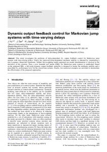
In this study, the state initial value of the system is 𝑥 = 𝑇 [−2.5 2.4 −17.5 2.4] for 𝜗(0) = 0. The multiple timedelays are selected as 𝜏1 and 𝜏2 . Figure 1 shows the responses of the control inputs. Figures 2 and 3 show the responses of 𝑥1 , 𝑥2 , 𝑥3 , and 𝑥4 with multiple time-delays 𝜏1 and 𝜏2 . From the three figures, we can see that the proposed method is effective and can stabilize the closed-loop system quickly.

10

Mathematical Problems in Engineering 240

20

160

10

80

0

0

−10

−80

−20

−160

0

2

4

6 Time (s)

8

10

12

u1 u2

−30

0

2

4

6 Time (s)

8

10

12

x3 x4

Figure 3: The response curves of state variables 𝑥3 and 𝑥4 .

Figure 1: The response curves of control input. 20

state property (converge exponentially). Furthermore, we have extended the results to the general nonlinear case. Finally, the simulation results illustrate the effectiveness of the main results. As further work, the proposed methodology will be extended to more complex control problems, such as 𝐻-∞ control of fuzzy affine systems with actuator faults.

10

0

−10

Conflicts of Interest

−20

The authors declare that there are no conflicts of interest regarding the publication of this paper.

−30

Acknowledgments 0

2

4

6 Time (s)

8

10

12

x1 x2

Figure 2: The response curves of state variables 𝑥1 and 𝑥2 .

This research was financially supported by National Natural Science Foundation of China (Project no. 61473248); Natural Science Foundation of Hebei Province of China (Project no. F2016203496); National Intellectual Property Office of China (Grant nos. ZL-2012-1-0052200.2, Zl-2012-1-0052199.3, and Zl-2014-2-0411083.9); and China National Heavy Machinery Research Institute.

6. Conclusions

References

This paper addresses the dynamic output feedback compensation control problem for a class of discrete system with multiple time-delays and uncertainties. The dynamic compensation controller is constructed and the control design conditions are relaxed, while the difficulty of the system design is decreased, it is easy to implement the system performance. With the developed nonlinear Lyapunov-Krasovskii functional, we have obtained sufficient conditions for the existence of output feedback controller such that the closedloop system is globally exponentially stable and achieves a prescribed level. The adaptive control law is designed such that the closed-loop systems have better stable state property (arbitrary small region of convergence) and better transient

[1] C. Hwang and Y.-C. Cheng, “A note on the use of the Lambert 𝑊 function in the stability analysis of time-delay systems,” Automatica, vol. 41, no. 11, pp. 1979–1985, 2005. [2] K. Eunro, I. Yang, and D. Lee, “Time-delay robust nonlinear dynamic inversion for chaos synchronization with application to secure communications,” Automatica, pp. 1–9, 2015. [3] U. Munz, C. Ebenbauer, T. Haag, and F. Allgower, “Stability analysis of time-delay systems with incommensurate delays using positive polynomials,” IEEE Transactions on Automatic Control, vol. 54, no. 5, pp. 1019–1024, 2009. [4] Z. Wang and H. Hu, “Robust stability test for dynamic systems with short delays by using Pade approximation,” Nonlinear Dynamics, vol. 18, no. 3, pp. 275–287, 1999.

Mathematical Problems in Engineering [5] Y. Wei, J. Qiu, and S. Fu, “Mode-dependent nonrational output feedback control for continuous-time semi-Markovian jump systems with time-varying delay,” Nonlinear Analysis. Hybrid Systems, vol. 16, pp. 52–71, 2015. [6] L. Li and Y. Jia, “Non-fragile dynamic output feedback control for linear systems with time-varying delay,” IET Control Theory & Applications, vol. 3, no. 8, pp. 995–1005, 2009. [7] Y. Lv, Z. Li, and Z. Duan, “Adaptive output-feedback consensus protocol design for linear multi-agent systems with directed graphs,” in Proceedings of the 27th Chinese Control and Decision Conference, CCDC 2015, pp. 150–155, chn, May 2015. [8] Y. Wei, J. Qiu, and H. R. Karimi, “Reliable output feedback control of discrete-time fuzzy affine systems with actuator faults,” IEEE Transactions on Circuits Systems-I Regular Papers, vol. 64, no. 1, pp. 170–181, 2017. [9] H. Feng and B.-Z. Guo, “On stability equivalence between dynamic output feedback and static output feedback for a class of second order infinite-dimensional systems,” SIAM Journal on Control and Optimization, vol. 53, no. 4, pp. 1934–1955, 2015. [10] J. Qiu, G. Feng, and H. Gao, “Fuzzy-model-based piecewise 𝐻∞ static-output-feedback controller design for networked nonlinear systems,” IEEE Transactions on Fuzzy Systems, vol. 18, no. 5, pp. 919–934, 2010. [11] Q. Wang and C. Wei, “Decentralized robust adaptive output feedback control of stochastic nonlinear interconnected systems with dynamic interactions,” Automatica, vol. 54, pp. 124– 134, 2015. [12] Y. Zhu, M. Krstic, and H. Su, “Adaptive output feedback control for uncertain linear time-delay systems,” IEEE Transactions on Automatic Control, vol. 62, no. 2, pp. 545–560, 2016. [13] B. Zhou, “Observer-based output feedback control of discretetime linear systems with input and output delays,” International Journal of Control, vol. 87, no. 11, pp. 2252–2272, 2014. [14] J. Qiu, G. Feng, and H. Gao, “Static-output-feedback H∞ control of continuous-time T-S fuzzy affine systems via piecewise lyapunov functions,” IEEE Transactions on Fuzzy Systems, vol. 21, no. 2, pp. 245–261, 2013. [15] R. Yang, P. Shi, G.-P. Liu, and H. Gao, “Network-based feedback control for systems with mixed delays based on quantization and dropout compensation,” Automatica, vol. 47, no. 12, pp. 2805–2809, 2011. [16] J. Yao, Z. Jiao, and D. Ma, “Extended-state-observer-based output feedback nonlinear robust control of hydraulic systems with backstepping,” IEEE Transactions on Industrial Electronics, vol. 61, no. 11, pp. 6285–6293, 2014. [17] C. Xia, B. Ji, and Y. Yan, “Smooth speed control for lowspeed high-torque permanent-magnet synchronous motor using proportional-integral-resonant controller,” IEEE Transactions on Industrial Electronics, vol. 62, no. 4, pp. 2123–2134, 2015. [18] S.-L. Chen, “Nonlinear smooth feedback control of a three-pole active magnetic bearing system,” IEEE Transactions on Control Systems Technology, vol. 19, no. 3, pp. 615–621, 2011. [19] S. Aouaouda, M. Chadli, M. T. Khadir, and T. Bouarar, “Robust fault tolerant tracking controller design for unknown inputs T-S models with unmeasurable premise variables,” Journal of Process Control, vol. 22, no. 5, pp. 861–872, 2012. [20] R. Toscano and P. Lyonnet, “Robust static output feedback controller synthesis using Kharitonov’s theorem and evolutionary algorithms,” Information Sciences. An International Journal, vol. 180, no. 10, pp. 2023–2028, 2010.

11 [21] B. Xian, M. S. de Queiroz, D. M. Dawson, and M. L. McIntyre, “A discontinuous output feedback controller and velocity observer for nonlinear mechanical systems,” Automatica, vol. 40, no. 4, pp. 695–700 (2005), 2004. [22] S. Chae and S. K. Nguang, “SOS based robust H fuzzy dynamic output feedback control of nonlinear networked control systems,” IEEE Transactions on Cybernetics, vol. 44, no. 7, pp. 1204– 1213, 2014. [23] Y. Wei, J. Qiu, H. R. Karimi, and M. Wang, “New results on dynamic output feedback control for Markovian jump systems with time-varying delay and defective mode information,” Optimal Control Applications and Methods, vol. 35, no. 6, pp. 656–675, 2014. [24] C.-C. Hua and X.-P. Guan, “Smooth dynamic output feedback control for multiple time-delay systems with nonlinear uncertainties,” Automatica, vol. 68, pp. 1–8, 2016. [25] X. Yuan, Z. Chen, Y. Yuan, and Y. Huang, “Design of fuzzy sliding mode controller for hydraulic turbine regulating system via input state feedback linearization method,” Energy, vol. 93, pp. 173–187, 2015. [26] S.-H. Chen and L.-C. Fu, “Output feedback sliding mode control for a stewart platform with a nonlinear observer-based forward kinematics solution,” IEEE Transactions on Control Systems Technology, vol. 21, no. 1, pp. 176–185, 2013. [27] C.-C. Hua, Q.-G. Wang, and X.-P. Guan, “Memoryless state feedback controller design for time delay systems with matched uncertain nonlinearities,” IEEE Transactions on Automatic Control, vol. 53, no. 3, pp. 801–807, 2008. [28] Y. He, G. P. Liu, D. Rees, and M. Wu, “Improved stabilisation method for networked control systems,” IET Control Theory and Applications, vol. 1, no. 6, pp. 1580–1585, 2007. [29] Y. He, M. Wu, G.-P. Liu, and J.-H. She, “Output feedback stabilization for a discrete-time system with a time-varying delay,” IEEE Transactions on Automatic Control, vol. 53, no. 10, pp. 2372–2377, 2008.

Advances in

Operations Research Hindawi Publishing Corporation http://www.hindawi.com

Volume 2014

Advances in

Decision Sciences Hindawi Publishing Corporation http://www.hindawi.com

Volume 2014

Journal of

Applied Mathematics

Algebra

Hindawi Publishing Corporation http://www.hindawi.com


Volume 2014

Journal of

Probability and Statistics Volume 2014

The Scientific World Journal Hindawi Publishing Corporation http://www.hindawi.com


Volume 2014

International Journal of

Differential Equations Hindawi Publishing Corporation http://www.hindawi.com

Volume 2014

Volume 2014

Submit your manuscripts at https://www.hindawi.com International Journal of

Advances in

Combinatorics Hindawi Publishing Corporation http://www.hindawi.com

Mathematical Physics Hindawi Publishing Corporation http://www.hindawi.com

Volume 2014

Journal of

Complex Analysis Hindawi Publishing Corporation http://www.hindawi.com

Volume 2014

International Journal of Mathematics and Mathematical Sciences


Journal of

Mathematics Hindawi Publishing Corporation http://www.hindawi.com

Volume 2014


Volume 2014

Volume 2014


Volume 2014

#HRBQDSDĮ,@SGDL@SHBR

Journal of

Volume 201


Discrete Dynamics in Nature and Society

Journal of

Function Spaces Hindawi Publishing Corporation http://www.hindawi.com

Abstract and Applied Analysis

Volume 2014


Volume 2014


Volume 2014

International Journal of

Journal of

Stochastic Analysis

Optimization



Volume 2014

Volume 2014