Dynamic scenario concept models - CRISMA project

Dynamic scenario concept models Alexander Garcia-Aristizabal, Maria Polese, Giulio Zuccaro (AMRA) Miguel Almeida, Valeria Reva, Domingos Xavier Viegas (ADAI) Tony Rosqvist, Markus Porthin (VTT)

31.8.2013

28.8.2013 | i

The research leading to these results has received funding from the European Community's Seventh Framework Programme FP7/2007-2013 under grant agreement no. 284552 "CRISMA“

42.1

Deliverable No. Subproject No.

4

Work package No.

42

Models for MultiSectorial Consequences Cascade Effects on Work package Title Crisis-Dependent Space-Time Scales Alexander Garcia-Aristizabal, Maria Polese, Giulio Zuccaro (AMRA) Miguel Almeida, Valeria Reva, Domingos Xavier Viegas (ADAI) Tony Rosqvist, Markus Porthin (VTT) F CRISMA_D421_final_public PU

Subproject Title

Authors

Status (F = Final; D = Draft) File Name Dissemination level (PU = Public; RE = Restricted; CO = Confidential)

Contact

[email protected] [email protected]

Project Keywords Deliverable leader

www.crismaproject.eu Multi-risk analysis; scenarios of cascading effects; concept model of dynamic scenario assessment Name: Alexander Garcia-Aristizabal Partner:

Contractual Delivery date to the EC Actual Delivery date to the EC

AMRA

Contact: [email protected] 31.08.2013 31.08.2013

http://www.crismaproject.eu

28.8.2013 | ii

Disclaimer The content of the publication herein is the sole responsibility of the publishers and it does not necessarily represent the views expressed by the European Commission or its services. While the information contained in the documents is believed to be accurate, the authors(s) or any other participant in the CRISMA consortium make no warranty of any kind with regard to this material including, but not limited to the implied warranties of merchantability and fitness for a particular purpose. Neither the CRISMA Consortium nor any of its members, their officers, employees or agents shall be responsible or liable in negligence or otherwise howsoever in respect of any inaccuracy or omission herein. Without derogating from the generality of the foregoing neither the CRISMA Consortium nor any of its members, their officers, employees or agents shall be liable for any direct or indirect or consequential loss or damage caused by or arising from any information advice or inaccuracy or omission herein.


28.8.2013 | iii

Table of Contents TABLE OF CONTENTS ................................................................................................................ III LIST OF FIGURES ......................................................................................................................... V LIST OF TABLES ......................................................................................................................... VII GLOSSARY OF TERMS ............................................................................................................. VIII EXECUTIVE SUMMARY ............................................................................................................... IX 1.

INTRODUCTION ................................................................................................................... 1

2.

STATE OF THE ART IN MULTI-RISK ASSESSMENT: A FRAMEWORK FOR CASCADING EFFECTS ........................................................................................................ 3 2.1. Multi-hazard and multi-risk assessment initiatives......................................................... 5 2.2. Multi-hazard assessment .............................................................................................. 6 2.3. Multi-risk assessment ................................................................................................... 8

3.

CONCEPT MODEL FOR DYNAMIC SCENARIO ASSESSMENT DUE TO CASCADE EVENTS .............................................................................................................................. 11 3.1. Concept model description ......................................................................................... 11 3.1.1. Contextualization within the CRISMA framework ............................................. 12 3.1.2. Integration of the cascading effects into the general framework of CRISMA .... 15 3.1.3. Concept model the dynamic scenario assessment due to Cascading effects .. 16 3.2. Identification and definition of the possible scenarios of cascading effects.................. 22 3.2.1. Setting of the area of interest (target system characterization) ........................ 22 3.2.2. Logic for scenario identification ....................................................................... 23 3.2.3. Example using the L’Aquila pilot case ............................................................. 25 3.3. Development of necessary databases: Scenarios and transition matrices .................. 27 3.3.1. Database of cascading effects scenarios......................................................... 27 3.3.2. Repository of transition matrices ..................................................................... 27

4.

DESCRIPTION OF METHODS FOR THE PROBABILISTIC ASSESSMENT ...................... 28 4.1. Examples of practical applications following those approaches described .................. 29 4.1.1. Analysis of databases of past events............................................................... 29 4.1.2. Use of physical models.................................................................................... 32 4.1.3. Use of Expert Elicitation .................................................................................. 35

5.

CONCLUSIONS AND RECOMMENDATIONS .................................................................... 37


28.8.2013 | iv

6.

REFERENCES .................................................................................................................... 40

APPENDIX (A) FITTING A PROBABILITY MODELS TO CASCADING EVENT CHAINS – IMPLEMENTATION USING BAYESIAN NETWORKS. ....................................................... 46


28.8.2013 | v

List of Figures Figure 1: Schematic description of the MRA procedure (from Marzocchi et al., 2012). .................. 12 Figure 2: Structure of the general framework of the CRISMA tool for DSS. ................................... 14 Figure 3: Concept model of the CRISMA platform considering cascading effects. ........................ 15 Figure 4: Concept model of the CRISMA platform considering cascading effects. Simplified version of the concepts presented in Figure 3 following the scheme for the general framework of CRISMA presented in Figure 2. .................................................................................................... 16 Figure 5: Logic for the damage assessment considering the cascading effects within the CRISMA concept model. The triggering event, is an event happening at a given time that is likely to produce a chain of adverse events. The direct effects of the triggering event (assessed e.g., using the CRISMA platform), are assessed in order to compute the direct consequences. Using the information from the database of cascading effects and the respective transition matrices (TM), the expected consequences of the chains of events can be quantified. ................. 17 Figure 6: Generic example of a transition matrix. .......................................................................... 18 Figure 7: Structure of the concept model for the dynamic scenario assessment due to cascading effects. .......................................................................................................................................... 19 Figure 8: Integration of decision nodes within an event-tree like structure representing cascading effects. ......................................................................................................................... 20 Figure 9: Example of the integration of decision nodes in the concept model for the dynamic scenario assessment due to cascading effects. ............................................................................ 21 Figure 10: An influence diagram representing scenarios of cascading events and some mitigation actions. ......................................................................................................................... 21 Figure 11: Example of system characterization in the target exposed area of interest................... 22 Figure 12: Scenario structuring following a 'Forward logic' approach: (a) definition of main triggering events; (b) for each triggering event identified, the sequence of triggered events is defined. ......................................................................................................................................... 24 Figure 13: Structure following a backward logic: after the definition of the outcome of interest (i.e. the effect), the model is built backwards exploring the most likely paths towards the initiating events. ............................................................................................................................ 24 Figure 14: Example of a diagram of cascading events identified for the case of an earthquake as the triggering event................................................................................................................... 26 Figure 15: Natural events causing NaTech hazards (data from 920 accidents recorded in the ARIA base over the period 1992 to 2012)(from: French Ministry for sustainable development – DGPR / SRT / BARPI http://www.aria.developpementdurable.gouv.fr/ressources/ft_natech_risks.pdf). ........................................................................... 30 Figure 16: (a) Fault geometry, epicenter (shown as a star), and location of the stations (triangles) where velocity seismograms were simulated (b) close-up image of the city showing the seismogram locations (from: Teramo et al., 2008)................................................................... 32 Figure 17: the 3D prototype structure assumed for seismically designed RC buildings in Italy (from Teramo et al., 2008). ........................................................................................................... 33


28.8.2013 | vi

Figure 18: Percentage of buildings exceeding (a) limit state 1 (LS1, slight damage) (b) limit state 2 (LS2, extensive damage) and (c) limit state 3 (LS3, collapse) (from: Teramo et al., 2008). ........ 33 Figure 19: Probability of occurrences (a) and landslide hazard levels (b) for a first hazard modelling scenario (specific parameters of water table level and landslides extension). (from: Olivier et al., 2011). ....................................................................................................................... 34 Figure 20: The Delft ‘classical’ expert weighting procedure (from: Aspinall, 2006). ....................... 36 Figure 21: Basic connection types. ............................................................................................... 47 Figure 22: Initial BN used for the landslide susceptibility assessment. The initial network is a naive BN, the landslide is the root node, and each landslide-causing factor is a child node of the landslide (from: Song et al., 2012). ............................................................................................... 49 Figure 23:Resulting structure of Bayesian networks for the landslide-susceptibility assessment (from:Song et al., 2012). ............................................................................................................... 49


28.8.2013 | vii

List of Tables Table 1: The conditional probability table of the node lithology (from:Song et al., 2012)................ 50


28.8.2013 | viii

Glossary of terms Term Domino effect

Cascade effect Serial domino (cascade) effect Parallel domino (cascade) effect World state

Multi-hazard

Multi-risk

Cascading effect scenario Decision tree

Decision node

Transition matrix

Database of scenarios

Definition "a cascade of events in which the consequences of a previous accident are increased by following one(s), as well spatially as temporally, leading to a major accident“ (Delvossalle, 1996) “the situation for which an adverse event triggers one or more sequential events (synergetic event)” (Marzocchi et al., 2009) “Happening as a consequent link of the only accident chain caused by the preceding event” (Reniers et al., 2004) “Happening as one of several simultaneous consequent links of accident chains caused by the preceding event” (Reniers, 2004) A particular status of the world, defined in the space of parameters describing the situation in a crisis management simulation, that represents a snapshot (situation) along the crisis evolvement. The change of world state, that may be triggered by simulation or manipulation activities by the CRISMA user, corresponds to a change of (part of) its data contents. To determine the probability of occurrence of different hazards either occurring at the same time or shortly following each other, because they are dependent from one another or because they are caused by the same triggering event or hazard, or merely threatening the same elements at risk without chronological coincidence. To determine the whole risk from several hazards, taking into account possible hazards and vulnerability interactions (a multi-risk approach entails a multi-hazard and multi-vulnerability perspective). a synoptical, plausible and consistent representation of a series of actions and events, in which an adverse event triggers or interacts with one or more sequential events Decision support tool that uses a tree-like graph or model of decisions and their possible consequences, including chance event outcomes, resource costs, and utilities. Element of a decision tree which represents a decision (e.g., to assess different possible mitigation actions) to be taken in a particular segment of a decision tree. A matrix-like representation of the conditional probabilities P(IM2|IM1), indicating the probability that a triggered event with intensity IM2 occurs given the occurrence of a triggering event with intensity IM1 A collection of plausible scenarios of cascading effects


28.8.2013 | ix

Executive Summary This deliverable (D42.1) is the output of the CRISMA project. First, a general overview of the state of the art in multi-hazard and multi-risk assessment is presented. This information is useful for contextualize the cascading effects problem within the general framework of the multi-risk. The core of the document is the presentation of the concept model for the dynamic scenario assessment due to cascading effects, and the strategy to integrate it into the general CRISMA DSS tool. The conceptual model for considering cascading effects presented here follows a clear and transparent sequential logic that starts in the identification of scenarios of cascading effects, and then provides the concepts useful to quantify the expected damages for a given specific scenario. The sequential logic is very specific for scenario-based assessments; this is in fact the key element in order to integrate the cascading effects model within the CRISMA tool. The proposed model is based on the use of two fundamental concepts: (1) a database of cascading scenarios, and (2) a repository of transition matrices. For each of these two fundamental concepts, strategies for gathering the required information are also provided. In fact, an extensive discussion is presented for illustrating possible strategies for the identification and structuring of cascading scenarios. Likewise, the specific problem of quantifying the probabilities required for the transition matrices is another complex factor highlighted and discussed in the text. In many cases it may require different kinds of expertise, and the use of different sources of information. In order to provide a general view on the possible strategies that can be used in order to quantify these probabilities, in this document we discuss different possible approaches that can be explored in order to quantify probabilities required for the hazard and risk assessment.


28.8.2013 | 1

1. Introduction One of the main characteristics of CRISMA system is its ability to deal with different hazards in one single tool. The inclusion of the cascading effects issue in this tool adds a new set of advantages to the use of CRISMA system as it allows to assess the effects of two or more different hazard events since they are trigger related. In this perspective, the present deliverable describes the concept model for dynamic scenario assessment due to cascade events that will be implemented in the CRISMA system and which will be applied and more deeply developed in the future deliverables D42.2 (Almeida et al., 2013) and D42.3 (Almeida et al., 2014). The present deliverable also covers a description of existing multi-risk assessment methods that are being used or developed around the world. This deliverable (D42.1) starts with the discussion of the most important methods and concepts in multi-risk assessment, which are derived from reviewing the most important past and on-going projects and scientific publications in which the multi-risk, multi-hazard, and cascading effects problem has been approached. The complexity of the cascade effects requires the application of a proper risk assessment methodology. In the common practice, the risk evaluation is done for independent events where single risk indexes are determined. However, when considering the cascading events, the resulting risk indices may be higher than the simple aggregation of single risk indexes. For this reason the multi-risk assessment should be carried out taking into account all the possible interactions of risks due to cascading effects. Recent works have provided detailed literature reviews of the most important initiatives on multi-hazard and multi-risk assessment. This deliverable summarizes and complements the main results obtained by these initiatives, in particular, from the European projects MATRIX (e.g., Garcia-Aristizabal and Marzocchi, 2012a, b) and ARMONIA (e.g., Del Monaco et al., 2007), as well as the papers of Marzocchi et al. (2012) and Kappes et al. (2012). It should be mentioned that different terminology was used in the practice of risk evaluation when addressed to the concept of chain reaction effect. The term “domino effect” is mainly applied in studies of accidents in the chemical and process industry triggered by technological or natural disasters (Delvossalle, 1996; Reniers et al, 2004), while the term “cascade effect” is mainly used in studies of natural disasters triggered by natural disasters in the context of multi-risk assessment (Marzocchi et al., 2009). The outputs presented in this deliverable, have the main objective of developing the “concept model” of dynamic scenarios due to cascade events including the effects of time dependent mitigation actions, as well as the strategy for integrating them into the CRISMA general tool. In this way, this deliverable describes the structure and the theoretical framework of the concept model for the CRISMA platform introducing the dynamic scenario mechanism to consider cascading effects assessments. Quantitative risk analyses considering cascading effects require a clear identification of possible scenarios of cascading events and approaches to quantify probabilities associated to each scenario. The logic for both scenario identification and structuring of the cascading effects scenarios is presented in this document. Furthermore, the effects of time dependent mitigation actions were also included into the concept model throughout the definition of decision nodes. Possible approaches that can be explored in order to quantify probabilities required for the hazard and risk assessment are also described, including some examples of past cases considering cascades of natural and Na-Tech (technological hazards triggered by natural events) events.


28.8.2013 | 2

The cascading effects analysis will be integrated as a transversal system in the CRISMA tool that can be activated at any time by the users. In this way, the user may activate the cascading effect tool using the input data and the results of the models that drive to the situation in which the cascading effect analysis become necessary to run (i.e., a given triggering event occurring at a given time).


28.8.2013 | 3

2. State of the art in multi-risk assessment: a framework for Cascading Effects There is growing evidence that natural or man-made disasters can trigger other disasters leading to tremendous increase of fatalities and damages. In the last decade, cascade effect was an object of numerous studies. At the European Community level, particular attention was given to technological hazards triggered by natural events (NaTech hazards). Seveso I (82/501/EEC), Seveso II (98/82/EC) and SEVESO III (12/18/EU) Directives are addressed to both manmade and NaTech risk through rules regulating lifeline systems operations such as electrical power plants, gas and oil pipelines, water resources, and other industrial facilities with a high risk of accident. In the field of “natural-natural” hazards, most of studies were addressed to probabilistic assessment of landslides triggered by rainfall, earthquake, and typhoon (Guzzetti et al., 1999; Dai et al., 2001, 2004, 2011; Saha et al., 2005; Dahal et al., 2008a, 2008b; Dai and Lee, 2003; Ayalew and Yamagishi, 2005; Ohlmacher and Davis, 2003; Can et al., 2005; Wang et al., 2005; Yesilnacar and Topal, 2005; Chang et al., 2007; Garcia-Rodriguez et al., 2008; Chong et al., 2012). In the field of risk analysis of NaTech hazards, most of case studies involve industrial accidents caused by earthquakes, floods or lightning (Antonioni et al., 2007, 2009; Young et al., 2004; Renni et al., 2009, 2010; Kadri et al., 2012; Kadri and Châtelet, 2012; Abdolhamidzadeh et al., 2011). The assessment and mitigation of the impacts of hazardous events considering cascade effects require innovative approaches, which allow comparison and interaction of different risks for all the possible cascade events. A multi-risk approach is aimed to solve a problem of the interaction among different threats and to establish a ranking of the different types of risk taking into account possible cascade effects. The growing need to develop multi-risk approaches has led to the development of different projects in Europe and in different countries with the aim to provide tools and procedures for a successful planning and management of territory, and to homogenize existing methodologies within a unique approach. Some of the most relevant European Projects are: TEMRAP – The European multi-hazard risk assessment project (FP4, 1998– 2000). It aimed to develop an integrated methodology on multi-hazard and global risk assessment, on the basis of different experiences carried out in several European countries on natural disasters. EXPLORIS – Explosive eruption risk and decision support for EU populations threatened by volcanoes (FP5, 2002–2005). Addressed to quantitative analysis of explosive eruption risk in densely populated EU regions and the evaluation of the likely effectiveness of possible mitigation measures (such as land-use planning, engineering interventions in buildings, emergency planning and community preparedness) through the development of volcanic risk facilities, such as supercomputer simulation models, vulnerability databases, and probabilistic risk assessment protocols, and their application to high-risk European volcanoes. NA.R.As. – Natural risk assessment harmonisation of procedures, quantification and information (FP6, 2004–2006). Contribute to harmonise the risk assessment procedures and indicate ways to quantitative evaluation of hazard and risk levels.


28.8.2013 | 4

ARMONIA – Applied multi Risk Mapping of Natural Hazards for Impact Assessment (FP6, 2004–2007). Addressed to integration/optimisation of methodologies for hazard/risk assessment for different types of potentially disastrous events, and to harmonisation of different risk mapping processes for standardizing data collection/analysis, monitoring, outputs and terminology for end users (multi-hazard risk assessment); IRASMOS – Integral Risk Management of Extremely Rapid Mass Movements (FP6, 2005–2007). Reviewing, evaluating, and augmenting methodological tools for hazard and risk assessment extremely rapid mass movements (landslideand snow-avalanche disasters). ENSURE – Enhancing resilience of communities and territories facing natural and na-tech hazards (FP7, 2008–2011). Structure vulnerability assessment models: different aspects of physical, systemic, social and economic vulnerability will be integrated as much as possible in a coherent framework. CLUVA – Climate change and Urban Vulnerability in Africa (FP7, 2010–2013). Assessment of the environmental, social and economic impacts and the risks of climate change induced hazards expected to affect urban areas at various time frames (floods, sea-level rise, storm surges, droughts, heat waves, desertification, storms and fires). MATRIX – New Multi-Hazard and Multi-Risk Assessment Methods for Europe (2010–2013). Challenge multiple natural hazards and risks in a common theoretical framework. Development of a virtual city to allow simulation a wider number of different characteristic situations that exist in European countries. The multi-risk concept refers to a complex variety of combinations of risk, and, for this reason, it requires a review of existing concepts of risk, hazard, exposure and vulnerability, within a multi-risk perspective. A multi-risk approach entails a multi-hazard and a multivulnerability perspective. The multi-hazard concept may refer to (1) the fact that different sources of hazard might threaten the same exposed elements (with or without temporal coincidence), or (2) one hazardous event can trigger other hazardous events (cascade effects) that is the main issue of this deliverable. On the other hand, the multi-vulnerability perspective may refer to (1) a variety of exposed sensitive targets (e.g. population, infrastructure, cultural heritage, etc.) with possible different vulnerability degree against the various hazards, or (2) time-dependent vulnerabilities, in which the vulnerability of a specific class of exposed elements may change with time as consequence of different factors (as, for example, wearing, the occurrence of other hazardous events, etc.). Most if not all of the initiatives on multi-risk assessment have developed methodological approaches that consider the multi-risk problem in a partial way, since their analysis basically concentrate on risk assessments for different hazards threatening the same exposed elements. Within this framework, the main emphasis has been towards the definition of procedures for the homogenization of spatial and temporal resolution for the assessment of different hazards related to cascading effects. For vulnerability instead, being a wider concept, there is a stronger divergence over its definition and assessment methods; considering physical vulnerability issues, a more or less generalized agreement on the use of vulnerability functions (fragility curves) has been reached, which facilitate the application of such a kind of multi-risk analysis, however, for other kinds of vulnerability assessment (e.g. social, environmental, etc.) it is less clear how to integrate them within a multi-risk framework.


28.8.2013 | 5

Following the definitions provided in the working paper on “Risk assessment and mapping guidelines for disaster management” of the European Union (European Commission, 2010), the concept of “multi-hazard assessment” may be understood as the process “to determine the probability of occurrence of different hazards either occurring at the same time or shortly following each other, because they are dependent from one another or because they are caused by the same triggering event or hazard, or merely threatening the same elements at risk without chronological coincidence”. On the other hand, the definition provided in the same document for “multi-risk assessment” is: to determine the whole risk from several hazards, taking into account possible hazards and vulnerability interactions (European Commission, 2010). It is important here to point out the concept of “multi-hazard risk” assessment, often found in literature which, following the definition provided by Kappes et al. (2012) refers to the risk raised from multiple hazards and contrasts with the term multi-risk because the latter would relate also to multiple vulnerabilities and risks such as economic, ecological, social, etc. From the definitions provided in the previous paragraph, it can be outlined that a multi-risk approach entails a multi-hazard and multi-vulnerability perspective. This includes the following possible events: Events occurring at the same time or shortly following each other, because they are dependent on one another or because they are caused by the same triggering event or hazard; this is mainly the case of “cascading events”; or, Events threatening the same elements at risk (vulnerable/exposed elements) without chronological coincidence. In the following sections, a brief description of the state-of-the-art on multi-hazard and multi-risk assessment as derived from literature review is presented. For a more detailed description, the reader is invited to consult MATRIX project (Garcia-Aristizabal and Marzocchi, 2012a, b), ARMONIA project (Del Monaco et al., 2007), as well as the papers of Marzocchi et al. (2012) and Kappes et al. (2012).

2.1. Multi-hazard and multi-risk assessment initiatives A multi-hazard and multi-risk analysis consists of a number of steps and poses a variety of challenges. A multitude of methodologies and approaches is emerging to cope with these challenges, each with certain inherent advantages and disadvantages. Whatever approach is chosen, it has to be adjusted according to the objectives (e.g., which results are required?) and to the inherent issues (e.g., stakeholder interests), respectively (Kappes et al., 2012). Thus, the adjustment of the whole framework toward the aspired result, considering the inherent issues, is a fundamental necessity. Hence, right from the beginning, several principal choices have to be made: (1) the first major choice is the definition of the kind of analysis, namely, multi-hazard risk or multi-risk. This does not only depend on the research objective, but is also a question of data availability; (2) furthermore, it has to be decided the terms of the expected outcome, i.e., whether a qualitative, semi-quantitative, or quantitative outcome is needed. Based on the different reviews of different methods and concepts performed in the main documents cited before, different points can be outlined for the multi-hazard and multi-risk practices as seen from the bibliography. These main points are summarized in the following sections.


28.8.2013 | 6

2.2. Multi-hazard assessment The concept of “multi-hazard” is in general found in applications in which the main objective is the assessment of risk derived from different natural and man-made hazardous events. However, as found in the available literature, this concept has different connotations and for this reason it seems that it is understood in a different way according to the kind of specific application in which it is used. The most common kind of applications in which a kind of multi-hazard assessment is performed is found in projects in which this concept is assumed as the assessment of different hazards threatening the same area (or exposed elements). On the other hand, terms as ‘triggering effects’, ‘domino effects’ or ‘cascading failure’ are frequently used, but usually without a proper definition and without any deeper explanation of what they exactly refer to (GarciaAristizabal and Marzocchi 2012a). Despite the apparent confusing interpretations that exist around what is exactly understood for multi-hazard assessment, most of the procedures dealing with multi-risk analysis identify this concept as a fundamental factor to be considered in a holistic assessment of the risk. Nevertheless, a basic and rigorous methodology allowing defining a guideline for multi-hazard assessment has not been clearly proposed up to now. Considering this definition and the different nature of the multi-hazard initiatives found in literature, Garcia-Aristizabal and Marzocchi (2012a) have sorted the main approaches in function of the kind of application in which the multi-hazard concept has been applied. In this way, the following approaches were identified: (1) Multi-hazard seen as the assessment of different independent hazards that threaten a common area or common exposed elements; (2) Multi-hazard seen as the assessment of triggering, domino, or cascade effects and (3) Multi-hazard seen as the assessment of possible hazard interactions (at vulnerability level). Multi-hazard seen as the assessment of different independent hazards that threat a common area or common exposed elements. From this perspective, Garcia-Aristizabal and Marzocchi (2012a) described two major kinds of applications. First, those in which the main effort was oriented towards the harmonization of the hazard assessment process. In this case, the initiatives concentrate their main effort to define a common assessment strategy for the quantification of different hazards, for example, in probabilistic or qualitative terms, using indices, etc. The second kind of applications are those in which the main objective of the multi-hazard problem is to try to perform an integral assessment of the damage probability of a given exposed element, i.e., the damage probability (or rate) assessed as the sum of the probable damage that any specific hazard can independently produce in the exposed element of interest. This perspective may be a subset of the first since it implies a harmonization of the hazard assessment, however, the main effort here has been done in the identification of a set of mutually exclusive (i.e. cannot happen simultaneously) and collectively exhaustive (i.e. all potential events) critical events that may produce damage to the specific exposed element, so it is oriented specifically towards risk assessment problems. Examples of initiatives classified within this category are the NATHAN world map of natural hazards (MunichRe, 2011), the TIGRA project (Del Monaco et al., 1999), the TEMRAP project (European Commission, 2000), the ESPON project (Schmidt-Thomé, 2006), the ARMONIA project (Del Monaco 2007), etc.


28.8.2013 | 7

Multi-hazard seen as the assessment of possible interactions or cascading effects. The assessment of interactions is te core of a full multi-risk assessment. Examples of pionnering works trying to assess cascading effects are, e.g., the analysis of common triggering factors in TEMRAP project (European Commission, 2000), the development of “hazard interaction maps” in ESPON project, (Schmidt-Thomé, 2006), the Central American Probabilistic Risk Assessment (CAPRA) approach (CAPRA project), The Landslide hazard assessment proposed in the natural- and conflict-related hazards in Asia-Pacific project (OCHA, 2009), and in the field of man-made hazards there are examples as for industrial accidents triggered by earthquakes, floods and lightning (Kraussman et al., 2011). Finally, a probabilistic framework for the assessment of triggering effects has been proposed by Marzocchi et al. (2012). The domino effect was well studied in the context of the major accident hazards inside and outside the industrial sites in the scope of the requirement established by the European Community “Seveso-II” Directive (Directive 96/82/EC). In a more detailed analysis it is possible to consider two possible cases of interactions: (1) interactions at the hazard level, and (2) interactions at the vulnerability level (see e.g., Garcia-Aristizabal and Marzocchi 2012a, 2013). Interactions at the hazard level: From this perspective, the multi-hazard problem is understood as the assessment of possible ‘chains’ of adverse events in which, the occurrence of given initial ‘triggering’ events, entails a modification of the probability of occurrence of a secondary event. Even if this kind of problems can be assessed in a long-term basis, their utility can be highlighted in short-term problems. Interactions at the vulnerability level. This perspective of the multi-hazard problem basically intends to assess the effects that the simultaneous occurrence (or close in time) of two or more hazards may have for the final risk assessment. In this case, the action of different hazards is considered and combined at a vulnerability level, i.e., how the vulnerability of the exposed elements (to a given hazard) can be modified if simultaneously or in a short time window (in general short enough that the system cannot be repaired) another hazardous event takes place. Examples of this kind of hazard interaction at vulnerability level are found, for example in works as the fragility analysis of woodframe buildings considering combined snow and earthquake loading (Lee and Rosowsky, 2006), the seismic and volcanic interactions assessed in the work of impacts of explosive eruption scenarios at Vesuvius (Zuccaro et al., 2008, and EXPLORIS project, 2006), and in the multi-risk due to triggering effects developed in the NARAS project (Marzocchi et al., 2009) and in the MATRIX project (Marzocchi et al., 2012). All the possible interpretations that have emerged from the review presented in GarciaAristizabal and Marzocchi (2012a) demonstrate the ambiguity that this concept may represent if a full picture of the problem is not considered; in fact, as can be seen in the previous three points, the multi-hazard concept as found in literature imply different perspectives and consequently is applied to different kinds of applications. This fact may explain why a rigorous methodology for multi-hazard assessment does not exist. Even if we consider just a single perspective of those mentioned before, in some cases it is difficult to outline a methodological approach to generalize the specific problem.


28.8.2013 | 8

Kappes et al. (2012) outlined the following list of challenging points on multi-hazard assessment: Computation of the overall hazard due to multiple natural processes is difficult since the single processes are generally quantified in different units and measures. Typically, the development of a common standardization scheme (classification or indices, qualitative, or semiquantitative) is used to overcome this difficulty. The standardization procedure is a rather useful approach. Also, in the case of few input data, it is an adaptive method. However, it has to be kept in mind that due to the specificity of the scheme, it is only applicable for the aim it was developed for. If hazards are understood as interacting processes within geosystems, a new perspective has to be adopted. From this point of view, hazard relations might lead to hazard patterns that cannot be captured by summing up separate singlehazard analyses. Rather, multi-hazards can be assessed either by identification of coincidences (overlay) or by detailed scenario development.

2.3. Multi-risk assessment From the bibliographic review performed by Garcia-Aristizabal and Marzocchi (2012b), it emerges that most –if not all- of the initiatives on multi-risk assessment have developed methodological approaches that consider the multi-risk problem in a partial way, since their analyses basically concentrate on risk assessments for different hazards threatening the same exposed elements. Within this framework, the main emphasis has been towards the definition of procedures for the homogenization of spatial and temporal resolution for the assessment of different hazards. For vulnerability instead, being a wider concept, there is a stronger divergence over its definition and assessment methods; considering physical vulnerability issues, a more or less generalized agreement on the use of vulnerability functions (fragility curves) has been reached, which facilitate the application of such a kind of multi-risk analysis. However, for other kinds of vulnerability assessment (e.g. social, environmental, etc.) it is less clear how to integrate them within a multi-risk framework. In this framework the final multi-risk index is generally estimated as a simple aggregation of the single indices estimated for different hazards. Other approaches consider a single hazard at a time and multiple exposed elements (e.g. buildings, people, etc.) for the vulnerability, which are combined and weighted according to expert opinion and subjective assignment of weights. The choice of the methodology strongly depends on both the scale of the study and the availability of information (for hazard and vulnerability assessment). Worthy of note, many of the approaches found define theoretical frameworks for the multi-risk assessment that, when applied to real cases, are generally simplified. This is due to the difficulty to obtain the detailed information needed. It is also interesting to point out that many of the reports discuss the importance of the interaction among hazards and cascading of events for a fully multi-hazard perspective, however little effort has been made to define a rigorous methodology. Looking at the most important applications, it is evident that the methodological approach used is strongly determined by the scale of the study. For instance, if we consider the ‘large-scale’ methodologies, as for example The Disaster Risk Index - DRI (UNDP,2004), or the Natural Disaster Hotspots: A Global Risk analysis (Dilley et al., 2005), the multi-risk analysis is generally performed by the use of risk indices representing expected annual


28.8.2013 | 9

mortality and economic losses. A “total” risk index is estimated as a simple aggregation of single risks, and hazard or vulnerability interactions or cascade effects are not considered. This kind of result represents a synoptical methodology principally addressed to global policies with very low reliability at the local scale; the objective being to identify hotspots where natural hazard impacts may be largest. For example, Greiving (2006) described the Integrated Risk Assessment of Multi-Hazards, based on four components: (i) hazard maps; (ii) integrated hazard map; (iii) vulnerability map, and (vi) integrated risk map. This approach was elaborated in the context of the project “Spatial effects of natural and technological hazards in general and in relation to climate change”, constituted part of the European Spatial Planning Observation Network (ESPON, www.espon.lu). Hazard maps show where and with what intensity individual hazards occur. The individual hazard maps are aggregated to one integrated hazard map basing on the single hazard intensities; different weights are applied. Vulnerability map reflects the hazard exposure of an area (infrastructure, industrial facilities and production capacity, residential buildings as defined by the regional GDP per capita) and the human damage potential. Vulnerability and hazard indices are combined into aggregated risk map. As we go down in the scale of the analysis (e.g., regional to local scales), multi-risk assessment is generally based on more detailed analysis. For this kind of procedures, risk from different hazards is quantified either using a common metrics (in general expected mortality or economic losses in a given timeframe – normally 1 year), or based on normalized indices resulting from the grouping of hazard intensities and vulnerability degrees in generic classes (low to high). The results are generally expressed using risk curves or risk indices that, as result of homogenized analysis, may be ranked and allow direct risk comparison for different typologies of natural and man-made adverse events. Examples of applications in this group are The “Natural Risk Assessment” (NARAS) project (Marzocchi et al., 2009), the “Risque Naturel Transverse” (RISK-NAT) project (Carnec et al., 2005; Douglas, 2005, 2007), the comparative multi-risk assessments for the city of Cologne, Germany (Grunthal et al., 2006), the regional-level multi-risk project in the Piedmont region, Italy (Carpignano et al., 2009), the regional-level initiative of integration of natural and technological risks in Lombardy region, Italy (Lari et al., 2009), the multihazard risk assessment for the Turrialba city, Costa Rica (Van Westen et al., 2002), the Central American Probabilistic Risk Assessment (CAPRA) approach, and the ‘Regional RiskScape’ project in New Zealand: “Quantitative multi-risk analysis for Natural hazards: a framework for multi-risk modelling.” (Schmidt et al., 2011). The analysis performed of the state-of-the-art on multi-risk assessment from the different European and international initiatives described in Garcia-Aristizabal (2012b) highlighted the following main features and gaps for the multi-risk assessment: Different methodologies, ranging from simplified approaches to innovative and advanced methods, were identified in this state-of-the-art analysis. Nevertheless, practically all the reported studies present important problems when transformed into practical applications. For instance, any methodological approach for multi-risk assessment is strongly constrained by both data availability (for hazard and vulnerability assessment) and the scale of the problem. Multi-risk approaches may imply multiple hazards affecting the same exposed elements, and/or one or more hazard affecting different categories of exposed elements. In the first case, quantitative risk assessment is generally more viable since a common metric for loss assessment is easier to be defined (i.e. risk harmonization based on the harmonization of effects). In the second case,


28.8.2013 | 10

considering different categories of exposed elements (e.g. buildings, population, green areas, environmental, etc.) imply difficulties on both the definition of a common metric for loss assessment, and how to weight the different categories of exposed elements. This kind of analysis involves strong subjective decisions that are not always easy to justify, and the risk quantification is generally performed using normalized indices that may allow, for example, individuate hotspots of high risk to be identified. However, sometimes its utility for risk management and decision-making may be questionable. The most basic requisite for a quantitative multi-risk assessment is the definition of a target area, common time frame, a quantitative assessment of hazards (generally in probability terms), a coherent vulnerability assessment (i.e., linked to the intensity measure parameterizations adopted for the hazard assessment), and a defined metric to quantify losses. However, the choice of a specific kind of loss metric may present different problems and limitations. In fact, the effect of different hazards may have different temporal characteristics (e.g. the recovery of construction is not the same of that of agricultural land or trees). Also different return periods, for different hazards, may pose difficulties to integrate the cost over a given period of time. A strong limitation found up to now is that none of the analysed studies produce a rigorous methodology for multi-hazard assessment. Most of the multi-risk methodologies consider the effect of different hazards as independent, neglecting the possibility of hazard interaction or cascade effects. Worthy of note, many of the reviewed documents write comments about the importance that cascades of events or hazard interactions may have for the risk, but very few try to quantify some basic scenarios. Linked to the previous point, multi-risk assessment requires also a careful evaluation of the interaction between vulnerabilities to different hazards. For example, the seismic vulnerability of an edifice changes significantly if the roof is loaded by volcanic ash. Only very little effort has been devoted to tackle this issue. One of the main gaps found for the practical application of the more important quantitative multi-risk methodologies found in literature is the lack of fragility curves derived by intensity (of the hazardous event) vs. typology of exposed elements. This topic can be considered as one of the most significant matters to be addressed for future developments of multi-risk analysis, especially in highresolution analysis (at local scale). Another gap found is in the treatment of uncertainties. None of the methodologies consider uncertainty quantification at any step of the process (except for some specific hazard assessment approaches), nor propagate (epistemic) uncertainties up to the final risk values. The concept model for dynamic scenario assessment due to cascade events follows for the general procedure for considering interactions at the hazard and the vulnerability level reported by Marzocchi et al. (2012) and Garcia-Aristizabal and Marzocchi (2013).


28.8.2013 | 11

3. Concept model for dynamic scenario assessment due to cascade events In this section, we describe the concepts and the theoretical framework in order to develop the concept model for dynamic scenario assessment due to cascading effects for the CRISMA platform. The concept model described here has been built considering the general concept model of the CRISMA tool, so a considerable effort was done to define a structure as much as possible adaptable and implementable into that system. This chapter is structured as follows: the first section describes the structure and theoretical framework of the concept model for the CRISMA platform and introduces the dynamic scenario mechanism to consider cascading effects assessments. In the second section, we describe the logic for scenario identification and structuring. The third section describes the required databases that are necessary to be built in order to implement the system. Finally, the fourth section describes the mechanism to integrate decision nodes in order to provide capabilities to the system to take into account possible mitigation actions.

3.1. Concept model description The concept model for considering cascading effects into the dynamic scenario scheme of CRISMA has been designed to support scenario-based analyses. The concept of cascading effects in multi hazard assessment is a fundamental element in multi-risk problems. Considering long- and short-term assessments, Marzocchi et al. (2012) identify following main steps of the multi-risk assessment (MRA) procedure: (1) Definition of the space–time window for the risk assessment and the metric for evaluating the risks; (2) Identification of the risks impending on the selected area; (3) Identification of selected hazard scenarios covering all possible intensities and relevant hazard interactions; (4) Probabilistic assessment of each scenario; (5) Vulnerability and exposure assessment for each scenario, taking into account the vulnerability of combined hazards; and (6) Loss estimation and multi-risk assessment. In this framework, a set of scenarios correlating adverse events from different sources are defined. For each “risk scenario”, the chain of adverse events is defined in a series/parallel sequence of happenings through an “eventtree”. Each branch of the event tree is quantified by a probabilistic analysis considering the sequence of the events, the vulnerability and the exposed values of the specified targets. A schematic representation of the MRA process presented in Marzocchi et al. (2012) is shown in on Figure 1.


28.8.2013 | 12

Figure 1: Schematic description of the MRA procedure (from Marzocchi et al., 2012).

3.1.1. Contextualization within the CRISMA framework In CRISMA, the analysis of the cascading effects has to be intrinsically interrelated with the general concept model for the CRISMA tool. The concepts and definitions introduced in this section are a necessary introduction to frame the concept model for considering cascading effects. Nevertheless, note that it is a general summary of the Crisis Management conceptual model that is being developed in the CRISMA Project.


28.8.2013 | 13

With this consideration in mind, several terms (e.g. world, world state, etc.) shall be defined in the space of parameters describing the situation in a crisis management simulation. In the following, we explain contextually the structure of the general framework of the CRISMA tool and relevant terms that are introduced making reference to Figure 2. The complete explanation of the Concept model of the CRISMA tool, involving also other aspects as use cases and reference scenarios, as well as the description of the World State Analysis features, will be presented in the CRISMA deliverable D44.1 (Version 1 of Model for decision-making assessment, Economic impacts and consequences, and Simulation) that is being prepared and that will be released at month 20 (Broas et al., 2013). First of all, let’s consider that each analysis and consideration from the Decision Maker (DM), that is the CRISMA user, starts from the visualization of the a particular status of the world, as it may be represented and visualized in a GIS format, the so called world state WS (see glossary). The world in a generic sense (that is detailed in a world state with a particular set of data, as it will be explained next) shall contain all the basic territorial GIS information (e.g. costal lines, administrative boundaries, road network, housing, etc.). They are needed to visualize an area of interest, as well as all other geo-referenced databases that are either used as input for models or produced as result of modelling and that enable the calculation of useful Indicators for crisis management. Considering an Integrated System viewpoint (see section 3.1.3 in Kutschera et al., 2013) the structure of the world shall not change and is pre-defined once the simulation setup is performed. This means that, right from the initial setup of the crisis management simulation, it is possible to initialize the simulation session so that the world shall contain pre-defined sets of databases (for example seismic vulnerability classes distribution for buildings in the case of seismic impact simulation or flood vulnerability classes distribution in the case of flood impact simulation, etc.). In a Simulation Model Viewpoint, the world shall also contain the Simulation Model Control Parameters (SMCP), that are to be used to control the models in case a simulation based on world content is to be performed. The rationale to include the SMCP in the world will be explained while describing the world state. In addition, and also depending on the initial setup of the crisis management simulation (e.g. selected use case), attached to (and therefore included in) the world is a set of synthetic parameters, named Indicators, Criteria and Costs (ICC) that may be used by the DM in Multi-Criteria Analyses and/or Cost/Benefit analyses to have a more synthetic representation of the situation and be supported in taking decisions. In Figure 2 the initial world state, labelled with INPUT in the left panel of the Figure and happening at the time T0 (initial time), may be the collection of inventory data, meteorological data, as well as other input data that are provided to the system by the CRISMA user and/or retrieved through dedicated applications and web-services that are interfaced with the CRISMA platform. Note that the time T0 is time of the definition of the initial (current) representation of the World State in the area of interest. Starting from the input world state the DM can simulate the evolvement of the generic crisis in a generic phase (e.g. preparedness, response etc.) either by the use of simulation models driven by a change in model control parameters (also part of the world state), or through direct manipulation of the World State. This concept is represented in the upper part of Figure 2 under the “User interaction and Business Logic (for Manipulation and Simulation)” tag. The knobs drawn in each yellow box (upper part of Figure) are intended to represent the possible direct manipulation of World State data (referred to hazard, vulnerability, etc.) as well as the possible tuning of model control parameters for simulation with the use of selected models. The action of manipulation or simulation triggers a


28.8.2013 | 14

change (or transition, as indicated in Kutschera et al., 2013) of the World State (WS) to a new World State (WS’). Also time is considered as part of the world and it may change (with simulation or manipulation rules) in world state transitions. To represent the time dependency the generic world state is labelled with a subscript i (WSi, WS’i) with i referring to the time. USER INTERFACE AND BUSINESS LOGIC (FOR MANIPULATION AND SIMULATION) EXPOSURE: • Distrib. of people • Distribution of vulner. classes of buildings....

INPUT WORLD STATE (GIS)

Simulation model control parameters

Data 1

Model 1

………..

Model n

Data n

ICC Functions or models

Indicators, Criteria and Costs (ICC)

T0

RESOURCES MANAGMENT: • Ambulance • Fire Depart. • ...............

CHOICE of OUTPUT: • Analyses C/B • Multi-criteria Analysis • ...........

BLACK BOX

(MODEL REQUIRED)

Data 2

…………

MITIGATION: • Increase of build. resistance • Evacuation • ...........

BLACK BOX

WS ’ 1 WS ’’1 control WS’’’1

Simulation model Simulation model control parameters Simulation model control parameters parameters Data 1

Data 1 Data 1 Data 2 Data 2 Data 2

(MODEL REQUIRED)

Model 1

…

………… ………… …………

………..

Model n

Indicators, Criteria ..… Indicators, Criteria … Criteria andIndicators, Costs (ICC) and Costs (ICC) and Costs (ICC)

WS’n WS’’n WS’’’n

Simulation model control Simulation model control parameters Simulation model control parameters parameters Data 1

Data 1 Data 1 Data 2 Data 2 Data 2

………… ………… …………

Data n Data n Data n

Data n Data n Data n


DECISION


World State Analysis

HAZARD: • Event characeriz. (Intensity, return period, probab., location etc.)… • ………..

Indicators, Criteria Indicators, Criteria Criteria andIndicators, Costs (ICC) and Costs (ICC) and Costs (ICC)

T1

Tn

Figure 2: Structure of the general framework of the CRISMA tool for DSS.

Within this concept, the models are represented as “black boxes” (see orange boxes in figure); it means that their particular business logic is not of interest for the CRISMA tool, except for the required input data (that need to be part of the world state WS prior to simulation) and the output data (the results that need to be part of world state WS’ after simulation). Note that the Simulation Model Control Parameters (SMCP) need to be set at the beginning of each simulation activity leading to the change of a WS. The importance of attaching SMCP to the WS becomes evident when the need of comparing different WS’s deriving from different simulations arises. In fact, proceeding from left to right in Figure 1, it may be noted that starting from a single initial WS, several alternative world states may be determined (e.g. WS’1, WS’’1, WS’’’1….) at each time stamp. The variation between alternatives depends on the choices made by DM while setting determined SMCP to fixed values or by selected manipulation activities. In order to check the decision making process, the DM has to compare alternatives. To this aim, he/she may be supported by visualization of the status of alternative world states as it may be synthetically represented by selected relevant Indicators and Criteria, as well as Costs (ICC), describing the “status” of a situation (purple boxes). Also, DM may be supported by the World State Analysis, that is an additional feature of CRISMA allowing for multi-criteria and/or cost/benefit analysis and that suitably combines ICC according to standard rules. ICC are automatically determined and appended to the world, using dedicated ICC functions or models, and depend on the GIS information and databases (describing the world) and on SMCP. More detailed descrptions of the CRISMA concept


28.8.2013 | 15

model can be found in other deliverables, namely D24.1 (Criteria for the use in CRISMA), and D44.1, which treat more specifically ICC and the World State Analysis rules. 3.1.2. Integration of the cascading effects into the general framework of CRISMA The CRISMA model relies on the concepts world, world state (situation) and on a transition between world states that is driven either by events, by model outputs and/or by user manipulation. Within this framework, cascading effects are integrated as sequences of triggered events following an initial ”triggering event” occurring at a given time and affecting the world state (WS) at that given time. Figure 3 shows the general structure of the CRISMA concept model including the elements of cascading effects highlighted using green colours. Notice that the cascading effects are transversal to the sequence of events that are presented in the CRISMA concept. A simplified version of this figure following the general scheme for the conceptual model for the DSS system of CRISMA presented in Figure 2 is shown in Figure 4. There are three different concepts that are introduced for the integration of the cascading effects into the CRISMA framework: (1) the database of scenarios, (2) the transition matrix concept, and (3) the assessment and update of the expected impacts. These concepts are described in Section 3.1.3. The database of scenarios is the first element to be built. In fact, it constitutes a known element in the world state at time T0. The possible strategies for building a scenarios database are described in Section 3.2. Intrinsically related to the database of cascading scenarios, a repository of transition matrices should exist for the scenarios that are going to be quantified.

Figure 3: Concept model of the CRISMA platform considering cascading effects.


28.8.2013 | 16

Figure 4: Concept model of the CRISMA platform considering cascading effects. Simplified version of the concepts presented in Figure 3 following the scheme for the general framework of CRISMA presented in Figure 2.

3.1.3. Concept model the dynamic scenario assessment due to Cascading effects The main elements of the concept model considering cascading effects are generically represented in Figure 3, which can be used to describe the logic behind the conceptual model for the dynamic scenario assessment due to cascading effects. The “world state” at time T0 is represented in the first “world state” box. The database of cascading effects is represented in a green box. The scope of the cascading effects database is to communicate to the system the possible cascading scenarios that can be developed after the occurrence of a given event at a given time. Note that the DM can decide to study only some cascading events chains, and he/she can properly select them from the available Database, or can choose to perform the entire risk analysis (if the necessary information is available). To this aim an additional box “Cascading effects” is added in the upper part of the diagram in Figure 4, evidencing the simulation and manipulation features. When a given event happens, let’s say for example an earthquake, the pre-defined models in the CRISMA tool (working as “black boxes” into the systems) calculate and propagate spatially and temporally the intensities of the given event into the area of interest. For example, in the case of an earthquake, it creates the “shake maps” showing the distribution of the intensity measure selected for the analyses, as for example the acceleration of the ground motion. The model also combines the fragility models and the databases of exposed elements in order to calculate the maps of the expected impacts (due to the direct effect of the first event). This concept is described in Figure 5 where the direct consequences (damages) of a triggering event are represented along the vertical arrow running out of the “triggering event” box. Note that the triggering chains of “natural events” follow a horizontal flow in Figure 5, whereas the chains that are triggered after damages in the area of interest (generically denominated “triggered anthropic hazards” in Figure 5) are developed in the vertical direction.


28.8.2013 | 17

At this point, the concept model for the cascading effects can be activated. The two fundamental pieces of information required to assess the effects of possible cascading effects are (1) the database of scenarios and (2) the transition matrix. Those elements are described in the following sections.

Figure 5: Logic for the damage assessment considering the cascading effects within the CRISMA concept model. The triggering event, is an event happening at a given time that is likely to produce a chain of adverse events. The direct effects of the triggering event (assessed e.g., using the CRISMA platform), are assessed in order to compute the direct consequences. Using the information from the database of cascading effects and the respective transition matrices (TM), the expected consequences of the chains of events can be quantified.

3.1.3.1.

Database of scenarios of cascading effects

The database of cascading effects contains all the information about the identified scenarios of cascading effects. The procedure to define scenarios can be considered as the first and fundamental step towards a quantitative risk analysis considering cascading effects. To achieve the required complete set of scenarios, different strategies can be adopted, and a rigorous procedure for this process is described in Section 3.2. The objective of defining a database of cascading effects it is to collect the information of all the possible sequences of events that potentially can be triggered after a given (triggering) initial event. In general, the database should provide the following information: A catalogue of scenarios, which are the series of events that can be triggered (in a cascade) after the occurrence of a given triggering event. For example: Earthquake -> Landslide -> Flood -> … Availability of quantitative data for each identified scenario. Not all the scenarios can be suitable of quantitative analyses. This can be due to different reasons, such as, for example, no data available, no models for theoretical analysis, or simply because the scenario is not of interest for the problem.


28.8.2013 | 18

With the possible scenarios of cascading events identified, the next element is to collect the probabilistic information necessary to quantify the expected damages produced by the potential cascading effects. This information is found on the repository of transition matrices. 3.1.3.2.

The Transition Matrix (TM) concept

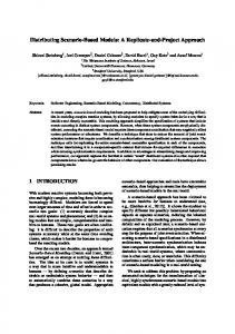
The transition matrix is a representation of the conditional probabilities of the form P(T1|E1), which means the probability of having the triggered event T1 given the occurrence of a triggering event E1). The structure of this element can be a N x M matrix, in which there are N classes of the intensity measures of the triggering event and M classes of intensity measure of the triggered event (Figure 6). When M or N are equal to 1 (just a binary case independent of the intensity of the triggered or triggering event), then the transition matrix will be a vector of values. Furthermore, if in both cases the conditional probability P(T1|E1) is independent of the intensities of the triggered and triggering events, then, P(T1|E1) will be represented by a scalar quantity.

Figure 6: Generic example of a transition matrix.

3.1.3.3.

Structure and representation of the concept model for cascading effects

From an operative point of view, the structure of the concept model for the dynamic scenario assessment due to cascading effects is illustrated in Figure 7. Considering the procedure for the assessment of the consequences and the evolution of the system, we can represent the problem running in three axes: The first one, running in the X direction (left to right), represents the time, which is the same time running in the world state defined in the concept model of CRISMA. Along this direction, T=0 is the current time, or in general, the time at which the world state is represented before the occurrence of any adverse event, or before starting any simulation. The Z axis (up-down) represents the assessment of the direct consequences (impacts, damages) due to the occurrence of the events in time (not considering cascading effects), whereas the Y axis (Normal to the page surface in the plane XZ) represents the assessment of expected consequences due to the cascading effects after the occurrence of a given triggering event in time. We can consider this axis as running also in sequence after the occurrence of a given triggering event.


28.8.2013 | 19

Figure 7: Structure of the concept model for the dynamic scenario assessment due to cascading effects.

In practice, the sequence of events happening in time are represented along the X axis, so it includes all the events for which the general CRISMA concept model is used in order to assess the direct consequence of these events (Z axis). So, the plane defined between the X and Z axes are in fact the representation of the evolution of the CRISMA concept model without considering the cascading effects analyses. When a given event occurs at a given time, let’s say, T1, from the database of scenarios and using the repository of transition matrices, the cascading effects concept model is activated in order to calculate the expected consequences due to those chains of events and producing an updated version of the maps of expected damages. It is worth noting that, in a case in which an event is effectively triggered, it will automatically be transposed into the XZ plane as a new event effectively happening into the sequence of events in time. In this way, the model can dynamically perform assessments of expected damages due to cascading effects and update the current world state after the occurrence of one or more events in time. 3.1.3.4.

Integration of decision nodes: a strategy to consider mitigation actions

The next point of interest to be discussed within the framework of the concept model for considering cascading effects in the CRISMA system is the possibility to assess mitigation actions. Those actions may be conceptualized, within the concept model for dynamic scenario assessment due to cascading effects, through the definition of decision nodes. The decision nodes are one of the key elements of decision tree. A decision tree is a decision support tool that uses a tree-like graph or model of decisions and their possible consequences, including chance event outcomes, resource costs, and utilities. In decision analysis, a decision tree and the closely related influence diagrams are used as visual and analytical decision support tools, where the expected values (or


28.8.2013 | 20

expected utility) of competing alternatives are calculated. The decision nodes are one of the elements of the decision trees, along with the chance and end nodes. As described in Section 3.1, the structure for the cascading effects is built on an event-tree like scheme, in which each of the nodes is quantitatively represented by a conditional probability. The integration of decision nodes within such a kind of logic is straightforward. In the segments in which decisions can be done in order to modify the outcome of the assessment (for example, mitigation actions), then a decision node can be included in order to assess the different outcomes considering different decisions taken. This concept is illustrated in Figure 8. After a given initial triggering event (TRi), n different events can be triggered (E1, E2, …, En), whose occurrence probability is measured by the conditional probability P(En|TRi). Note that this concept is intrinsically correlated to that of the transition matrix. Between the level 2 and level 3 of the analysis in Figure 8, it is supposed that a decision node DNa can be introduced. In the example m different possible decision, with m different possible outcomes can be defined. In that case, the m possible outcomes can be assessed through the evaluation of the different ‘parallel’ paths that are derived after the DNa. Following the representation shown in Figure 7, the different paths after a decision node can be represented as different alternatives in the Y direction of the figure, as shown in Figure 9. The differences of the outputs in the different parallel paths after the decision nodes shown in Figure 8 and Figure 9 constitute the elements to assess the effects of the different decision taken in the process (for example, mitigation actions).

Figure 8: Integration of decision nodes within an event-tree like structure representing cascading effects.


28.8.2013 | 21

Figure 9: Example of the integration of decision nodes in the concept model for the dynamic scenario assessment due to cascading effects.

A decision tree can be represented, for example, as an influence diagram (ID), focusing the attention on the issues and relationships between events. ID contains in addition to probabilistic nodes also decision and value nodes. Figure 10 shows an example of an influence diagram considering cascading events and mitigation. An initiating event, e.g. an earthquake, will cause some damage, but its effects can be influenced by the mitigation and prevention actions. This kind of analysis can be framed also in the general procedure for the identification and structuring of the scenarios of cascading effects (section 3.2).

Figure 10: An influence diagram representing scenarios of cascading events and some mitigation actions.


28.8.2013 | 22

3.2. Identification and definition of the possible scenarios of cascading effects The procedure to define scenarios can be considered as the first and fundamental step towards a quantitative risk analysis considering cascading effects. To achieve the required complete set of scenarios, different strategies can be adopted. In the proposed approach for CRISMA, the following logical flow of activities are proposed: Setting and clear definition of the area of interest. Choice of the most adequate ‘logic’ for scenario identification and structuring The details of these two steps are described and discussed in the following sections. 3.2.1. Setting of the area of interest (target system characterization) The first task is the clear definition of the area of interest (i.e., the place and systems where the ‘effects’ are going to be assessed), and the characterization of the systems of interest for the analysis. It means that the area of interest for the analysis is well known, all the components of the system are recognized, and roughly, an idea of the ‘success’ scenario is clear (i.e. we have a clear idea of the ‘desired situation’). For the characterization of the ‘target’ area, we can define the area of interest using for example a system ‘hierarchy’ or a functional decomposition, going from the most general definition to more detailed components. In this way the elements in the target area are decomposed into the fundamental subsystems of interest. For example, let’s suppose that our target area is a specific city. Then, we can highlight the specific characteristics of that city specifying the fundamental sub-systems that can be of interest in our analysis. Let’s suppose that in a given case we can identify the following sub-systems of interest: residential areas, a road network, distribution systems for electricity, water, and gas, and a generic industrial facility, as seen in Figure 11. Note that each sub-system can be also decomposed in its own sub-systems. In this perspective, it is possible to clarify from the beginning the level of detail of the analysis.

Figure 11: Example of system characterization in the target exposed area of interest.


28.8.2013 | 23

After the definition of the target area and the characterization of the exposed elements, the other important element that should be ‘a priori’ defined is the ‘metric’ for the quantification of the effects: it can be in terms of, for example, human fatalities, economic losses, loss of functionality, etc. Note that the metrics for quantification of the effects should be defined compatibly with Indicators, Criteria and Costs, that are relevant parameters considered as input for the World State Analysis, allowing a situation assessment in the CRISMA concept. 3.2.2. Logic for scenario identification Once the target area and systems of interest have been clearly defined, a strategy for the identification of all the possible scenarios should be defined. The objective behind all the process is the identification of “what can go wrong”. To achieve this objective it is necessary to define an objective process of finding, organizing and categorizing the set of cascading effects scenarios. As such, it should include well-known standard methods of scenario identification as event trees and fault trees. Given the complexity and diversity of scenarios that can be derived, especially for the diversity of test cases considered in CRISMA, a unique single approach could represent a limitation and could not ensure an exhaustive exploration of potential scenarios. Then, the selection of a specific approach for scenario identification may be a case-specific problem. We consider that a good start point can be found among one of the following “logical” approaches: • Using “forward logic” approaches, as for example, event-tree like structures; • Using “Backward logic” approaches, as for example, fault-tree like structures; • Apply both approaches, and overlay them to identify the most exhaustive set of scenarios (or highlight the most important ones). 3.2.2.1.

The ‘forward logic’ strategy (top-down):

Using a ‘forward logic’ strategy implies to start identifying the possible initiating (triggering) events (natural and non-natural). This kind of approach will follow a forward logic in the sense that for each initiating event (e.g. a flood or an earthquake) it will identify the possible outcomes (endpoints), following an event-tree-like structure. In this event-tree-like structure, the nodes are uncertain or chance events; the model shows the sequence of chance events that can lead to desirable or undesirable outcomes. Nevertheless, from the beginning or in a second step it is possible to add ‘decision’ nodes controlled by decision makers (in this way it becomes a ‘decision tree’). An example of a sequence of events following this ‘forward logic’ approach is shown in Figure 12. 3.2.2.2.

The ‘backward logic’ strategy (bottom-up):

The backward logic strategy begins with and endpoint, outcome or result, and works backwards to find the most likely causes of the effect, following a fault-tree-like structure. This approach starts considering the effects that have been selected for the analysis (i.e. the objective(s) of the risk analysis and the ‘metric’ identified). As with the forward logic analysis, in this case the nodes are uncertain or chance events and the structure commonly focus on identifying the most likely path from an endpoint back to its originating events. Decision nodes can be also added (from beginning or in a second step). An example of the structure following a ‘backward structure’ is shown in Figure 13.


28.8.2013 | 24

Figure 12: Scenario structuring following a 'Forward logic' approach: (a) definition of main triggering events; (b) for each triggering event identified, the sequence of triggered events is defined.

Figure 13: Structure following a backward logic: after the definition of the outcome of interest (i.e. the effect), the model is built backwards exploring the most likely paths towards the initiating events.


28.8.2013 | 25

3.2.2.3.

Combination of both: an adaptive scenario structuring strategy

The strategy outlined in this section is based on the concept of adaptive hierarchical modelling. The idea is to iteratively use both, the forward logic and the backward logic approaches, and combine the results obtained in order to exhaustively identify all the relevant scenarios for the specific problem analysed. In practice, in this case the people involved in the scenario identification problem are split in two independent groups: the first one, which will perform an analysis based on forward logic, and the second one which will perform a backward logic analysis. It is important that both analyses are developed independently, since the union of both analyses will yield a more complete definition of scenarios and a deeper understanding of the problem. This strategy can provide a roadmap for scenario identification and tracking that accounts for the characteristics of both the root causes and the target. Note that it would be desirable that both analysis groups have a variety of skills, experience, and interests. The union of the outputs of the adaptive scenario identification process described in this section will highlight the most important paths from the initiating events up to the endpoints representing the effects. Further the completeness of the scenario identification process, the overlapped paths will indicate also the most likely paths that are those of most interest for quantification. This process can be performed iteratively up to the convergence to a clear and well established set of scenarios. 3.2.3. Example using the L’Aquila pilot case To briefly illustrate the scenario identification problem, we present some preliminary analyses for the L’Aquila pilot case (but in general it can be the case of a generic earthquake). In this specific case, we are interested on analysing scenarios of cascading effects due to the occurrence of an earthquake. It means that we are interested on a single, specific triggering event, so we consider that in this case a forward-logic analysis may be enough for the scenario identification. In our exercise, we joined a group of people with different backgrounds to discuss about the possible cascading effects after the occurrence of an earthquake in L’Aquila area. The resulting diagram is shown in Figure 14. The example has been developed in the hypothesis of considering economic losses connected to Direct Tangible Damage as the ‘metric’ for the quantification of the effects. Starting with an earthquake as triggering event, the possible “first order” triggered events are firstly considered. Each one of them may be seen directly as an effect and may also be responsible of triggering other (intermediate) events. For example, in the case shown in Figure 14, the earthquake may cause a damage to a bridge that is part of transport infrastructure (denoted as event damage to road/rail transport infrastructure in figure). If the bridge is near some buildings (it may happen in densely inhabited areas) its collapsing may induce damages on buildings. The building damage may be also induced directly by the earthquake, as evidenced in figure (second of the considered “first order” triggered events). The events following the event building damage may be grouped under the same identifying category (denoted in this example as Dam 2) and therefore, they are exemplified only once, and recalled with the same number if they occur after other first order or intermediate events. For example, the building damage due to bridge collapse, as described in the first case of the scheme, can be continued by considering the possible chain of events described in the second row (denoted with Dam 2) and so on.


28.8.2013 | 26

Figure 14: Example of a diagram of cascading events identified for the case of an earthquake as the triggering event.

In other words, any part of the diagram where Dam i appears, can be continued plugging in the chain that start with the same number identifying tag. In fact, after the building damage event (number 2) other triggered events may happen. Indeed, such event may cause the local rupture of the gas distribution system (denoted with damage to gas network, number 3). The latter event may drive to an explosion, that may cause further building or industrial facility damage, or triggering a fire (urban/wildfire, industrial or forest fire), and so on. Following the same logic, all the branches starting from each first-order triggered event are developed until arriving to the final events and effects.


28.8.2013 | 27

3.3. Development of necessary databases: Scenarios and transition matrices The concept model exposed in this section implies the definition of different databases. The first database that needs to be created is that of the scenarios of cascading effects. Then, for each of the scenarios of interest, a repository with the probabilistic information is necessary. That probabilistic information is organized on data structures that we denominate here as ‘transition matrices’. 3.3.1. Database of cascading effects scenarios The output of the process of identification and definition of the possible cascading effects scenarios (section 3.2), is a set of all the identified chains of adverse events that can be a priori identified. Generally, this exhaustive set of scenarios is often too complex, or in some cases the interest in the specific problem may be on analysing just a limited number of cases. Then, the database of scenarios to be considered into the system should highlight the subset of scenarios that are effectively of interest, and/or those for which quantification is possible because of data availability. The database of cascading effects should include the following information: The catalogue of scenarios: each scenario has to contain the full chain of events that were identified in the scenario identification phase. Identification of the specific scenarios for which quantification is of interest and data is available. Identification of the metric (and units) for the loss assessment (chosen between ICC), and the intensity measures defined for each kind of event in the chain. Those intensities have to be coherent with those used for the definition of the transition matrices. Each scenario selected for quantification has to be accompanied by its set of transition matrices. 3.3.2. Repository of transition matrices As described in Section 3.1.1, for the quantification of the expected damages for each scenario of cascading effects it is necessary to create a repository of transition matrices. The transition matrix contains all the probabilistic information that allows quantifying the specific chain in consideration. It relates the conditional probabilities of having a given intensity of the triggered event given the intensity of the triggering event. Furthermore, as described in Section 3.1.1, it can be an N x M matrix, a vector or a binary quantity, depending on the discretization of the intensity measures of both the triggered and triggering events. The repository of transition matrices has to be closely correlated with the database of scenarios. In fact, there should be one transition matrix for each node of the chain of events. The discretization reflected by the transition matrix has to be coherent with the intensity measures defined for the specific events analysed at each node. To populate the probability values into the transition matrices is the main scientific problem of the assessment of cascading effects. The values can be calculated using different sources of information, as for example databases of past events, using physical models, or based on expert opinion elicitations. Due to the importance of this issue, a detailed description of those possible approaches is presented in Section 4.


28.8.2013 | 28

4. Description of methods for the probabilistic assessment In this chapter we intend to outline some possible strategies that may be used in order to quantify the probabilities necessary in the hazard and risk assessment process and to populate the information required for the transition matrices of the conceptual model for cascading effects. The use of probabilistic methods for hazard and risk assessment is strongly conditioned on the availability of data and the complexity of the system under analysis. The use of databases of past events is the most straightforward approach used in practice to quantify hazards. In fact, hazard probabilities that include rate or recurrence analyses and frequency-magnitude relations may be derived from inventories of past events (when available). However, the use of historical data for the assessment of hazards may have some limitations. For example, the recorded data may be limited to event occurrences, not providing information about the intensity measures of interest for the hazard and risk assessment. On the other hand, databases containing information about the impacts of past events (e.g. the number of affected/injured/evacuated or homeless people, appeal for national/international assistance or level of damage/interruption of normal community life processes) may be recorded by different official entities using different methodologies and showing no homogeneous information. Furthermore, the degree and accuracy of recording may vary over time, what leads to uncertainties and consequently spatial and temporal limitations. Another important fact to be considered when analysing databases of past events is to check if the process shows non-stationary conditions. For example, due to the effects of climate change, in many cases climate-related hazards may be more correctly modelled using models accounting for non-stationary conditions (e.g., Makkonen et al., 2007; Garcia-Aristizabal et al., 2013). Examples of applications and methods for nonstationary analysis of extreme events can be found, for example, in Coles (2001), Katz et al. (2002), Ouarda and El-Adlouni (2011), Seidou et al. (2012). A specific application in multi-hazard assessment of non-stationary climate-related extremes using Bayesian methods for the model parameter estimation can be found in Garcia-Aristizabal et al. (2013). Under the lack of completeness in historical data, the use of physical modelling for the processes involved can be an useful and complementary approach to explain the genesis and dynamics of hazards, to understand triggering and triggered mechanisms, to propagate spatially and temporally the intensity measure(s) of interest and to use this information in order to calculate the probability of intensity measure exceedances. For example, physical modelling can be used to generate shake maps with the spatial distribution of the ground motion properties (e.g., acceleration) for the characteristic events (with given probability of occurrence) from the earthquake sources affecting the area of interest of a given analysis. In the case of landslides triggered by some external factors, physical modelling can be used to characterize geotechnical parameters contributing to slope stability, to model triggering factors in the studied area, and to estimate landslide probabilities in a given area of interest. In cases of uncertainty due to insufficient data, and when using physical (or empirical) modelling of the processes is not feasible (for example, because of lack of expertise, resources, or just not enough time available to perform it), the use of expert opinion elicitation procedures are valid alternatives able to provide accurate information to quantify probabilities in hazard and risk assessments. It is a formal, structured and documented process that provides means for a proper and full incorporation of the uncertainties


28.8.2013 | 29

represented by different technical interpretations. For this reason, expert elicitation has gained increasing acceptance, for example, in probabilistic seismic hazard analyses for critical facilities. From a quantitative point of view, all those different approaches described in the previous paragraphs require the quantification of probabilities. Those probabilities can be obtained whether using the classical (frequentist) or using Bayesian statistics. It is worth of note that the use of Bayesian methods can be a valid (and sometimes necessary) tool to be applied in those cases with few data or when using expert opinion techniques. The advantage of the Bayesian methods is that it may allow to integrate data from different sources (e.g., databases, or output from models and expert opinion elicitations) and to take into account both aleatory and epistemic uncertainties in the process (e.g., Marzocchi et al., 2012). More specifically, the use of Bayesian networks can be an interesting alternative to face problems of quantification of cascading effects. A description of the implementation and use of Bayesian networks can be found in Appendix A.

4.1. Examples of practical applications following those approaches described 4.1.1. Analysis of databases of past events Available historical data are important to assess the expected frequencies and the severity of hazard. Data collection and the construction of a spatial database, from which relevant factors will be extracted, are the main steps for hazard mapping and following assessment of the relationship between hazard and causative factors. The use of databases in the case of NaTech hazards. Major NaTech hazards, accidents in industrial facilities triggered by natural factors such as forest fires, runoff and floods, avalanches, hurricanes and tornadoes, storms, landslides and earthquakes, tsunamis, volcanic eruptions, lightning, occur mainly due to damage to process equipment resulting in loss of containment. Probabilistic assessment of NaTech hazards based on databases of past events may be exemplified by numerous studies undertaken for technological accidents following an earthquake, flood, or lighting (Antonioni et al., 2007, 2009; Young et al., 2004; Renni et al., 2009, 2010; Kadri et al., 2012; Kadri and Châtelet, 2012; Abdolhamidzadeh et al., 2011). The main sources of information for Natech hazard assessment are main European industrial-accident databases ARIA (2006), FACTS (2006), MARS (2008), MHIDAS (2001), TAD (2004), and US Response Centre´s database (NRC) database (2008). For instance, ARIA database has recorded 920 NaTech accidents occurred in France (747 events) and abroad (173 events) over the period 1992–2012 (Figure 15). The ARIA and NRC databases are publicly available. The MHIDAS, FACTS and TAD require a license. The MARS database contains confidential information on major accidents submitted to the European Commission.


28.8.2013 | 30

Figure 15: Natural events causing NaTech hazards (data from 920 accidents recorded in the ARIA base over the period 1992 to 2012)(from: French Ministry for sustainable development – DGPR / SRT / BARPI http://www.aria.developpement-durable.gouv.fr/ressources/ft_natech_risks.pdf).

Several studies indicate that lightning strike on equipment in storage and processing activities are the most common cause of accidents triggered by natural hazards. Lightning can affect industrial structure by direct strike, indirect lightning currents that induce secondary sparks, and by the disruption of control systems and electrical circuitry. Analysis of historical data allows identification of five equipment categories: (1) storage tanks, (2) flare stacks, (3) electrical and electronic equipment, (4) pipes, and (5) compressors and pumps, and probabilities of equipment damage (Renni et al., 2009, 2010). In the study of lightning-induced industrial accidents, 721 records were extracted from databases mentioned above: MARS – 4(0.6%); TAD – 9(1.2%); ARIA – 45(6.2%); MHIDAS – 79(11.0%); NRC – 584(81.0%). Data retrieved from the industrial accident databases were categorized by different criteria, such as loss of containment (and substances involved), industrial activity (and inventory involved), and accident scenario, what allows estimating the most frequent damages due to lightning. Concerning industrial activities involved in lightning-induced accidents with hazardous material release (190 accidental records), 125 (65.1%) accidents occur within petrochemical industry, 58 (30.1%) within Oil&Gas, 3 (1.6%) within pharmaceutical and fine chemicals, 3 (1.6%) within metallurgic and galvanic, and 3(1.6%) were related with other industrial activities. Among 485 (out of 721) accidental records regarding equipment, the following categories were identified: 289 (59.6%) were storage tanks, 64 (13.2%) flare stacks, 56 (11.5%) electrical and electronic equipment, 55 (11.3%) pipes, and 21 (4.4%) compressors and pumps. The analysis of 721 accident scenarios revealed that the majority of lightningtriggered accidents resulted in the release of hazardous substances which did not ignite or exploded (416 accidents, 57.7%); fires occurred in a third of the analysed cases (251 accidents, 34.8%), followed by explosion (51 accidents, 7.1%) and toxic cloud dispersion (3 accidents, 0.4%). From 335 (out of 721) registered accidents in which equipment damage led to a release of hazardous substances, high release (>1000kg) occur within 228 (37.7%) accidents, medium (100–1000kg) in 213 (35.3%) and low ( 30%).

Figure 19: Probability of occurrences (a) and landslide hazard levels (b) for a first hazard modelling scenario (specific parameters of water table level and landslides extension). (from: Olivier et al., 2011).

Phast, ALOHA and ANSYS software are some examples of tools for probabilistic assessment of the release of chemical substances: Phast (DNV, commercial software): Industry hazard analysis software tool to analyse situations which present hazards to life, property and the environment, and to quantify their severity. Hazard analysis of these scenarios: discharge and dispersion models, including DNV's proprietary Unified Dispersion Model (UDM);


28.8.2013 | 35

flammable models, including resulting radiation effects, for jet fires, pool fires and fireballs; explosion models, to calculate overpressure and impulse effects. Available models include the Baker Strehlow, TNO Multi-Energy and TNT explosion models, models for the toxic hazards of a release including indoor toxic dose calculations. ALOHA- Areal Locations of Hazardous Atmospheres (EPA-Environmental Protection Agency, free software) is a program designed to model chemical releases for emergency responders and planners. It can estimate how a toxic cloud might disperse after a chemical release and also features several fires and explosions scenarios. The program generates a variety of scenario-specific outputs, including threat zone plots, threats at specific locations, and source strength graphs (also threat zones on MARPLOT maps). ALOHA allows modelling of many release scenarios, such as toxic gas clouds, BLEVEs, jet fires, vapour cloud explosions, and pool fires. ANSYS Fluent (ANSYS Inc. commercial software), Fluid dynamics simulation in various applications. ANSYS Fluent software contains the broad physical modeling capabilities needed to model flow, turbulence, heat transfer, and reactions for industrial applications ranging from air flow over an aircraft wing to combustion in a furnace, from bubble columns to oil platforms, from blood flow to semiconductor manufacturing, and from clean room design to wastewater treatment plants. 4.1.3. Use of Expert Elicitation Expert elicitation is a tool for formalizing and quantifying of expert opinions on a subject where there is an uncertainty due to insufficient data for further use in decision making or forecast of event. It provides a set of possibilities based on the opinion of experts, and allows the quantification of the uncertainty concerning those opinions. Various elicitation procedures have been proposed (for example, Cooke method, Delft method, Delphy method, ERF model, Equal Weights model, for details see Flandoli et. al., 2011). Among those methods, the discrete testing method developed by Cooke (1991) is often known as the “classical” model. In this procedure, the experts respond to test questions with known answers. Different weights are computed (using a calibration and informativeness score) and attributed to individual experts to weight their answers to target questions (i.e., the objective of the elicitation excercise). The “Calibration score” characterizes the ability of an expert to be statistically accurate when assigning values to probability outcomes against known values, and the “Informativeness score” represents the expert’s capacity to provide concentrated distributions over the variables. Delft procedure, developed by Delft University of Technology, in The Netherlands, is another example of elicitation methodology that has been applied extensively as a decision support tool in many safety-critical risk assessment situations (Aspinall, 2006). Figure 20 illustrates the basis of the Delft ‘classical’ expert weighting procedure. The performance of a number of experts on a set of seed questions (test questions with known answers) leads to individual scoring weights. These weights are then used to linearly pool the experts’ distributional responses to produce a synthetic decision-maker outcome for the target question. There are several software tools designed to capture expert knowledge and support expert elicitation, such as Elicitator, SHELF or EXCALIBUR (Devilee and Knol, 2011).


28.8.2013 | 36

The Elicitator software (http://elicitator.uncertweb.org/) is used for eliciting judgements about prior structures in regression models and was built for applications in ecological modelling. It uses maps to give experts instantaneous feedback about the consequences of their judgements on the model in question. The SHeffield ELicitation Framework (SHELF) carries out elicitation of probability distributions for uncertain quantities from a group of experts. Finally, EXCALIBUR is a software that implements Cooke’s classical method for elicitation and opinion pooling.

Figure 20: The Delft ‘classical’ expert weighting procedure (from: Aspinall, 2006).

Note: The authors declare that they do not have any relation with all the commercial software or devises mentioned in this deliverable, and that there is no conflict of interest for any of them.


28.8.2013 | 37

5. Conclusions and recommendations This document contains very important information useful for the development of the CRISMA DSS tool. First, a general overview of the state of the art in multi-hazard and multi-risk assessment is presented. This information is useful for contextualize the cascading effects problem within the general framework of the multi-risk. A chapter with the description of the CRISMA conceptual model is presented in Section 3.1.1, and after that, the concept model for the dynamic scenario assessment due to cascading effects and the strategy to integrate it into the CRISMA general tool is presented in Sections 3.1.2 and 3.1.3. The following set of recommendations is mainly oriented to highlight the main critical points that can be found when putting in practice the concepts developed here (i.e, for the final users). Furthermore, it intends to highlight the main points that we foresee as important elements for moving forward from the creation of the conceptual model towards the practical implementation of the DSS system (i.e., for the developers). Conclusive remarks and recommendations for final users The conceptual model for considering cascading effects presented here follows a clear and transparent sequential logic that starts in the identification of scenarios of cascading effects, and then provides the concepts useful to quantify the expected damages for a given specific scenario. Note that the sequential logic is very specific for scenario-based assessments; this is in fact is the key element in order to integrate the cascading effects model within the CRISMA tool. In fact, when an event occurs at a given time ti, the CRISMA tool should activate two tasks: 1. It has to activate the routines for the quantification of the direct effects of the event occurring at time ti. It implies modelling of the propagation of the intensity of the hazard event, computing the expected damages in the target areas, etc. 2. It has to activate the module of the cascading effects, which basically means to explore into the database of scenarios to identify potential sequences of events, and when a final user selects a given scenario of interest, perform calculations using the databases of exposed elements and transition matrices. Finally, it has to update the maps of expected losses for the given scenario of interest. When an event in the cascade of events happens at time tn=ti+t’, it will become a new event in the CRISMA general tool, and from there, the two tasks defined in the previous point are again activated. This recursive behaviour allows moving forward in time in a dynamic link between primary events and triggered events. One of the main practical problems that has been identified for the implementation of the concept model presented here is the availability of data for the full implementation and quantification of the chains of events. The scenarios that can be identified at the beginning of the analysis can be extremely complex and involving a variety of interactions that can be overwhelming for computation. Then, we recommend concentrating the effort on identifying the most important scenarios (understood as those in which a significant amplification of the losses due to cascading effects is more likely to occur). In order to provide efficient tools for the scenario structuring and identification, we have included in this document the Section 3.2 in which some


28.8.2013 | 38

practical strategies commonly used in risk and reliability assessment of systems are exposed. The specific problem of quantifying the probabilities required for the transition matrices is another complex factor to take in consideration. In many cases it may require different kinds of expertise, and using different sources of information. In order to provide a general view on the possible strategies that can be used in order to quantify these probabilities, in Chapter 4 we discuss different possible approaches that can be explored in order to quantify probabilities required for the hazard and risk assessment. Some conclusive remarks that we can highlight are summarized as follows: 1. The first alternative to explore for the probabilistic analysis is of course to use the databases of past events. It may provide information about the occurrence probabilities of events in the different sources of interest. In some cases, it may contain information measured directly in terms of the intensity measures of interest. In this case, the database analysis may be enough for the probabilistic hazard assessment. Examples of this case can be found in many climaterelated hazards problems (e.g., extreme events of precipitation, wind, temperature, heat waves, etc.). 2. When the information from past events is limited to event occurrences and without directly measuring the intensities required for the risk assessment, an important tool that can be used to complement this information is by using physical or empirical modelling of the physical process involved for propagating the intensity measure from the source to the area of interest in which the exposed elements are located. This approach can be implemented by using one or more models using different parameterizations of the problem, and in that case the using of Bayesian techniques may provide an excellent framework to integrate the different sources of information. 3. An alternative approach to the physical modelling can be provided by the implementation of an “expert opinion” elicitation. This kind of approach can be particularly useful in problems in which few data is available for the specific problem under analysis, or also when there is not possibility to perform physical modelling of the processes. In this case, a pool of experts can be elicited in order to obtain information about the possibility of occurrence of some undesired event or about the effects after its occurrence. All those possible approaches can be complementary among them. To define which strategy is the better to be adopted in a given case depends on the specific characteristics of the problem, the availability of the data and into the capacity of performing modelling of the physical process. We consider that the procedure defined here is general enough to be directly applied to face a wide range of practical problems. Nevertheless, we cannot ensure that all the potential problems can be adapted to this strategy. Then, it is likely that some incompatibilities can be encountered when implementing the system and applying it to some specific cases or events in a chain of events. Alternative ways using qualitative analysis can be eventually an alternative strategy for extremely complex problems or poorly know processes. Recommendations for the next steps following the concept model development


28.8.2013 | 39

We consider that the next step after the definition of the conceptual model is the implementation of the system. This process inevitably has to be done in perfect coherence with the general tool under development in CRISMA. In fact, the CRISMA tool should be able to launch the cascading effects module identifying the scenarios after the occurrences of an event, and passing it to the system that has to handle them. Furthermore, the cascading effects model should read information from the output of other modules (i.e. the assessment of direct effects after the occurrence of the triggering event, model modules propagating hazard intensities, and so on.


28.8.2013 | 40

6. References Abdolhamidzadeh, B., Abbasi, T., Rashtchian, D. & Abbasi, S.A. 2011. Domino effect in processindustry – An inventory of past events and identification of some patterns. Journal of Loss Prevention in the Process Industries, Vol. 24, No 5, pp. 575–593. Almeida, M., Reva, V., Viegas, D.X., Garcia-Aristizabal, A., Polese, M., Zuccaro, G., Cabal, A., Coulet, C., Cossalter, A., Pilli-Sihvola, K., Poussa, L., Molarius, R. 2013. Database and Model for Dynamic scenario assessment V1. Deliverable D42.2 of the European Integrated Project CRISMA, FP7-SECURITY- 284552. Almeida, M., Ribeiro, L.M., Viegas, D.X., Garcia-Aristizabal, A., Zuccaro, G., Polese, M., Nardone, S., Marcolini, M., Cabal, A., Grisel, M., Coulet, C., Pilli-Sihvola, K. 2014. Database and Model for Dynamic scenario assessment V2. Deliverable D42.3 of the European Integrated Project CRISMA, FP7-SECURITY- 284552. Antonioni, G., Spadoni, G. & Cozzani, V. 2007. A methodology for the quantitative risk assessment of major accidents triggered by seismic events. Journal of Hazardous Materials No. 147, pp. 48– 59. Antonioni, G., Bonvicini, S., Spadoni, G. & Cozzani, V. 2009. Development of a framework for the risk assessment of Na-Tech accidental events, Reliability Engineering and System Safety No. 94, pp. 1442–1450. ARIA. 2006. Analyse, Recherche, et Information sur les Accidents. French ministry of ecology and sustainable development, bureau for analysis of industrial risk and pollution. http://www.aria.developpement-durable.gouv.fr/. Aspinall, W.P. 2006. Structured Elicitation of Expert Judgment for Probabilistic Hazard and Risk Assessment in Volcanic Eruptions. In: Mader H.M., Coles S.G, Connor C.B. and Connor L.J. (eds) Statistics in Volcanology. Special Publications of IAVCEI, 1. Geological Society, London. Ayalew, L. & Yamagishi, H. 2005. The application of GIS-based logistic regression for landslide susceptibility mapping in theKakuda-Yahiko Mountains, Central Japan. Geomorphology, No. 65, pp. 15–31. Broas, P., et al. (Eds), 2013. Version 1 of Model for decision-making assessment, Economic impacts and consequences, and Simulation. Deliverable D44.1 of the European Integrated Project CRISMA, FP7-SECURITY- 284552. CAPRA: Central www.ecapra.org

American

Probabilistic

Risk

Assessment

(CAPRA)

project.

Website:

Carnec, C., Modaressi, H., Douglas, J., Raucoules D. & Simonetto, E. 2005. Contribution of space imagery to vulnerability assessment of elements exposed to geological risks. TS14 Disaster II/General, 31st International Symposium on Remote Sensing of Environment: Global Monitoring for Sustainability and Security, St Petersburg, Russian Federation, 20-24 June. Carpignano, A., Golia, E., Di Mauro, C., Bouchon, S. & Nordvik J-P. 2009. A methodological approach for the definition of multi-risk maps at regional level: first application. Journal of Risk Research, Vol. 12, No.3-4, pp. 513-534. Can, T., Nefeslioglu, H.A., Gokceoglu, C., Sonmez, H.& Duman, T.Y. 2005. Susceptibility assessments of shallow earthflows triggered by heavy rainfall at three catchments by logistic regression analyses. Geomorphology No.72, pp. 250–271.


28.8.2013 | 41

Chang, K.T., Chiang, S.H. & Hsu M.L. 2007. Modeling typhoon- and earthquake-induced landslides in a mountainous watershed using logistic regression. Geomorphology No. 89, pp. 335– 347. Chen, S. H. & Pollino, C. A. 2012. Good practice in Bayesian network modelling. Environmental Modelling & Software, No. 37, pp. 134–145. Chong, X., Xiwei, X., Fuchu, D. 2012. Comparison of different models for susceptibility mapping of earthquake triggered landslides Computers & Geosciences, No. 46, pp. 317–329. Coe, J.A., Michael, J.A., Crovelli, R.A., Savage, W.Z., Laprade, W.T. & Nashem W.D. 2004. Probabilistic Assessment of Precipitation-Triggered Landslides Using Historical Records of Landslide Occurrence, Seattle, Washington, Environmental & Engineering Geoscience, Vol. X, No. 2, pp. 103–122. Coles. S. 2001. An introduction to statistical modeling of extreme values. Springer series in statistics, Springer-Verlag London limited. Cooke R.M. 1991. Experts in Uncertainty. NewYork: Oxford University Press; Dai, F.C., Lee, C.F., Li, J., Xu, Z.W. 2001. Assessment of landslide susceptibility on the natural terrain of Lantau Island, Hong Kong. Environmental Geology, No.40, pp. 381–391. Dai, F.C. & Lee, C.F. 2003. A spatiotemporal probabilistic modeling of storm-induced shallow landsliding using aerial photographs and logistic regression. Earth Surface Processes and Landform, No. 28, pp. 527–545. Dai, F.C., Lee, C.F., Tham, L.G., Ng, K.C. & Shum, W.L. 2004. Logistic regression modelling of storm-induced shallow landsliding in time and space on natural terrain of Lantau Island, Hong Kong. Bulletin of Engineering Geology and the Environment, Vol. 63, No. 4, pp. 315–327. Dai, F.C., Xu, C., Yao, X., Xu, L., Tu, X.B. & Gong, Q.M. 2011. Spatial distribution of landslides triggered by the 2008 Ms 8.0 Wenchuan earthquake, China. Journal of Asian Earth Sciences, Vol. 40, No. 4, pp. 883–895. Dahal, R.K., Hasegawa, S., Nonomura, A., Yamanaka, M., Dhakal, S. & Paudyal P. 2008a. Predictive modelling of rainfall-induced landslide hazard in the Lesser Himalaya of Nepal based on weights-of-evidence, Geomorphology, No.102, pp. 496–510. Dahal, R.K., Hasegawa, S., Nonomura, A., Yamanaka, M., Masuda, T. & Nishino, K. 2008b. GISbased weights-of-evidence modelling of rainfall-induced landslides in small catchments for landslide susceptibility mapping. Environmental Geology, Vol. 54, No. 2, pp. 314–324. Del Monaco, G., Margottini, C. & Serafini S. 1999. Multi-hazard risk assessment and zoning: an integrated approach for incorporating natural disaster reduction into sustainable development. TIGRA (The Integrated Geological Risk Assessment) Project (Env4-CT96-0262) Summary Report. Del Monaco, G., Margottini, C. & Spizzichino, D. 2007. Report on new methodology for multi-risk assessment and the harmonisation of different natural risk maps. Deliverable 3.1, ARMONIA project, contract 511208. Delvossalle, C. 1996. Domino Effects Phenomena: Definition, Overview and Classification. First European Seminar on Domino Effects. Leuven. Belgium, FederalMinistry of Employment, Safety Administration, Direction Chemical Risks, Brussels,Belgium, pp. 5-15. Devilee, J.L.A. & Knol, A.B. 2011. Software to support expert elicitation: An explorary study of existing software packages, RIVM Letter Report 630003001/2011. National Institute for Public Health and the Environment, Nederland.


28.8.2013 | 42

Di Carluccio, A., Iervolino, I., Manfredi, G., Fabbrocino, G.& Salzano E. 2006. Quantitative probabilistic seismic risk analysis of storage facilities, in: Proc. CISAP-2, Chem. Eng. Trans. No.9, p. 215. Dilley, M., Chen, R.S., Deichmann, U., Lerner-Lam, A.L., Arnold, M., (with: J. Agwe, P. Buys, O. Kjekstad, B. Lyon and G. Yetman), 2005. Natural Disaster Hotspots: A global risk analysis. The world Bank hazard management unit, Washington, D.C. Directive 96/82/EC. 1996. Council Directive 96/82/EC of 9 December 1996 on the control of majoraccident hazards involving dangerous substances. Official Journal of the European Communities, L 10/13 , Brussels, 14.1.97. Douglas, J. 2005. RISK-NAT (Module 4): Methods and tools for risk evaluation. Progress report. BRGM/RP-54041-FR. http://www.brgm.fr/publication/rapportpublic.jsp Douglas, J. 2007. Physical vulnerability modelling for natural hazards risk assessment. Natural Hazards and Earth System Sciences, Vol.7, No.2, pp. 283-288. http://www.nat-hazards-earth-systsci.net/7/283/2007/nhess-7-283-2007.html. European Commission DG XII, Environment and Climate Program. 2000. TEMRAP: The European Multi-Hazard Risk Assessment Project, contract ENV4-CT97-0589. European Commission, 2010. Commission staff working paper: “Risk assessment and mapping guidelines for disaster management”, Brussels, December 2010. EXPLORIS. 2006. Explosive Eruption Risk and Decision Support for EU Populations Threatened by Volcanoes (EXPLORIS). EU funded project, Contract No. EVR1-CT-2002-40026, 2002-2006. Fabbrocino, G., Iervolino, I., Orlando, F. & Salzano E. 2005. Quantitative risk analysis of oil storage facilities in seismic areas, J. Hazard. Mater. No.123, pp. 61–69. FACTS. 2006. Failure and Accidents Technical Information System. TNO Built Environment and Geosciences, The Netherlands. http://www.factsonline.nl. Fenton, N., Neil, M. & Marquez, D. 2008. Using Bayesian networks to predict software defects and reliability. JRR161 IMechE 2008 Proc. IMechE Vol. 222 Part O: J. Risk and Reliability. Flandoli, F., Giorgi, E., Aspinall, W.P. & Neri A. 2011. Comparison of an ewexpert elicitation model with the Classical Model, equal weights and single experts, using a cross-validation technique. Reliability Engineering and System Safety, No. 96, pp.1292–1310. Garcia-Aristizabal, A., Bucchignani, E., Palazzi, E., D'Onofrio, D., Gasparini, P. & Marzocchi, W. 2013. Analysis of non-stationary climate-related extreme events considering climate-change scenarios: an application for multi-hazard assessment in the Dar Es Salaam region, Tanzania. Submitted to Natural hazards, under review (2013). Garcia-Aristizabal, A. & Marzocchi, W. (main authors). 2013. Probabilistic methods for multi-hazard assessment. Deliverable D3.4 of MATRIX (New methodologies for multi-hazard and multi-risk assessment methods for Europe) project. Contract No. 265138 Garcia-Aristizabal, A. & Marzocchi, W. (main Authors). 2012a. Review of existing procedures for multi-Hazard assessment. Deliverable D3.1 of MATRIX (New methodologies for multi-hazard and multi-risk assessment methods for Europe) project. Contract No. 265138. Garcia-Aristizabal, A. & Marzocchi, W. (main authors). 2012b. State-of-the-art in multi-risk assessment. Deliverable D5.1 of MATRIX (New methodologies for multi-hazard and multi-risk assessment methods for Europe) project. Contract No. 265138.


28.8.2013 | 43

Garcia-Rodriguez, M.J., Malpica, J.A., Benito, B.& Diaz, M. 2008. Susceptibility assessment of earthquake-triggered landslides in El Salvador using logistic regression. Geomorphology, Vol. 95, No. 3–4, pp. 172–191. Gelman, A., Carlin, J.B., Stern, H.S. & Rubin, D.B. 1997. Bayesian Data Analysis. Chapman & Hall, London. Greiving, S. 2006. Integrated risk assessment of multi-hazards: a new methodology. Natural and technological hazards and risks affecting the spatial development of European regions. Geological Survey of Finland, Special Paper 42, pp.75–82. Grunthal, G., Thieken, A. H., Schwarz, J., Radtke, K., Smolka, A., & Merz, B. 2006. Comparative Risk Assessments for the City of Cologne – Storms, Floods, Earthquakes, Nat. Hazards, No.38, pp. 21–44. Guzzetti, F., Carrara, A., Cardinali, M. & Reichenbach, P. 1999. Landslide hazard evaluation: a review of current techniques and their application in a multi-scale study, Central Italy. Geomorphology, No. 31, pp. 181–216. Kadri, F., Châtelet, E. & Chenc, G. 2012. Method for quantitative assessment of the domino effect in industrial sites. Process Safety and Environmental Protection (article in press). Kadri, F. & Châtelet, E. 2012. Domino Effect Analysis and Assessment of Industrial Sites: A Review of Methodologies and Software Tools, International Journal of Computers and Distributed Systems, Vol 2, No.3, pp. 1-10. Kappes, M., Keiler, M., Elverfeldt, K. & Glade T. 2012. Challenges of analyzing multi-hazard risk: a review. Nat. Hazards, Vol. 64, No. 2, pp. 1925-1958. DOI 10.1007/s11069-012-0294-2. Katz, R., Parlange, M., Naveau, P. (2002) Statistics of extremes in hydrology. Advances in water resources 25(8-12):1287–1304. Korb, K. B. & Nicholson, A.E. 2010. Bayesian Artificial Intelligence, 2nd ed. CRC Press. Kraussmann, E., Renni, E., Campedel, M. & Cozzani, V. 2011. Industrial accidents triggered by earthquakes, floods and lightning: lessons learned from a database analysis. Nat. Nazards, No. 59, pp. 285-300. DOI 10.1007/s11069-011-9754-3. Kutschera P., Dihé P., Rannat K., Sommer M., Vandeloise Y., DeGroof A., Schlobinski S., Havlik D., Sautter J., Boži B., Deri O., Bracker H., Yliaho J., Scholl M., Engelbach W. 2013. ICMS Functional Architecture Document V1, Deliverable D32.1 of the European Integrated Project CRISMA, FP7-SECURITY- 284552. Lari, S., Frattini, P. & Crosta, G.B. 2009. Integration of natural and technological risks in Lombardy, Italy. Nat. Hazards Earth Syst. Sci., No. 9, pp. 2085–2106. Lee, K.H. & Rosowsky, D.V. 2006. Fragility analysis of woodframe buildings considering combined snow and earthquake loading. Structural Safety, Vol. 28, No.3, pp. 289-303. Makkonen, L., Ruokolainen, L., Räisänen, J. & Tikanmäki, M. 2007. Regional Climate Model Estimates for Changesin Nordic Extreme Events. Geophysica 43(1–2), 25–48. Marzocchi, W., Mastellone, M.L., Ruocco A.Di., Novelli, P., Romeo, E. & Gasparini, P. 2009. Principles of multi-risk assessment. Interaction amongst natural and man-induced risks. Project Report, FP6 SSA Project: Contract No. 511264. Marzocchi, W., Garcia-Aristizabal, A., Gasparini, P., Mastellone, M.L. & Ruocco, A.D. 2012. Basic priciples of multi-risk assessment: a case study in Italy, Nat Hazards DOI 10.1007/s11069-0120092-x.


28.8.2013 | 44

MHIDAS. 2001. Major Hazard Incident Data Service. Health and Safety Executive, United Kingdom. MARS. 2008. Major Accident Reporting System, European Commission, Joint Research Centre, Institute for the Protection and Security of the Citizen, Italy http://emars.jrc.ec.europa.eu. MunichRe. 2011: http://www.munichre.com (section Publications), NATHAN worldmap of natural hazards, 5th. Edition – last visited: June 2011. Murphy, K. 2012. Software Packages for Graphical Models / Bayesian Networks. web site. http://www.cs.ubc.ca/~murphyk/Software/bnsoft.html (accessed on 27.8.2012). Murphy, K. 2001. The Bayes Net Toolbox for MATLAB. Computing Science and Statistics, No. 33, pp.1024–1034. NRC. 2008. United States National Response Center Database. United States Coast Guard. http://www.nrc.uscg.mil/nrchp.html. OCHA – United Nations Office for Coordination of Humanitarian Affairs, OCHA regional office for Asia and the Pacific, 2009. Risk assessment and mitigation measures for natural and conflict related hazards in Asia-Pacific. Norwegian Geotechnical Institute (NGI) report 20071600-1. Ohlmacher, G.C. & Davis, J.C. 2003. Using multiple logistic regression and GIS technology to predict landslide hazard in northeast Kansas, USA. Engineering Geology, No. 69, pp. 331–343. Olivier, M., Sedan, O. & Monod B. 2011. Contribution of physical modelling to landslide hazard mapping: case of the French Basque coast. “The second world landslide forum, Rome: Italy (2011)” – Proceedings of the Second World Landslide Forum – 3-7 October 2011, Rome. Ouarda, T., & El-Adlouni, S. (2011) Bayesian nonstationary frequency analysis of hydrological variables. JAWRA Journal of the American Water Resources Association 47(3):496–505. Pradhan, B. & Lee, S. 2010a. Delineation of landslide hazard areas on Penang Island, Malaysia, by using frequency ratio, logistic regression, and artificial neural networks models. Environmental Earth Sciences, Vol. 60, No. 5, pp. 1037–1054. Pradhan, B. & Lee, S. 2010b. Regional landslide susceptibility analysis using backpropagation neural networks model at Cameron Highland, Malaysia. Land- slides, Vol. 7, No. 1, pp. 13–30. Pradhan, B. & Lee, S. 2010c. Landslide susceptibility assessment and factor effect analysis: backpropagation artificial neural networks and their comparison with frequency ratio and bivariate logistic regression modelling. Environmental Modelling and Software, Vol. 25, No. 6, pp. 747–759. Reniers, G., Dullaert, W. & Soudan, K. 2004. A Domino Effect Evaluation Model, University of Antwerp, Faculty of Applied Economics. Renni, E., Antonioni, G., Bonvicini, S., Gigliola, S. & Cozzani, V. 2009. A novel framework for the quantitative assessment of risk due to major accidents triggered by lightning, Chemical Engeneering Transactions, No.17, pp. 311-316. Renni, E., Krausmann E. & Cozzani V. 2010. Industrial accidents triggered by lightning, Journal of Hazardous Materials, No. 184, pp. 42–48. Saha, A.K., Gupta, R.P., Sarkar, I., Arora, M.K. & Csaplovics, E. 2005. An approach for GISbased statistical landslide susceptibility zonation — with a case study in the Himalayas. Landslides. No 2, pp. 61–69. Salzano E., Iervolino I. & Fabbrocino G. 2003. Seismic risk of atmospheric storage tanks in the framework of quantitative risk analysis, J. Loss Prevent Process, No. 16, pp. 403–409.


28.8.2013 | 45

Schmidt-Tomé, P., (Editor), Kallio, H., Jarva, J., Tarvainen, T., Greiving, S., Fleischhauer, M., Peltonen, L., Kumpulainen, S., Olfert, A., Schanze, J., Bärring, L., Persson, G., Relvão, A.M., Seidou, O., Ramsay, A., Nistor, I. 2012. Climate change impacts on extreme floods i: combining imperfect deterministic simulations and non-stationary frequency analysis. Natural Hazards pp 1– 13, DOI 10.1007/s11069-011-0052-x. Schmidt, J., Matchman, I., Reese, S., King, A., Bell, R., Henderson, R., Smart, G., Cousins, J., Smith, W. & Heron, D. 2011. Quantitative multi-risk analysis for natural hazards: a framework for multi-risk modelling, Nat. Hazards, No. 58, pp. 1169-1192. DOI 10.1007/s11069-011-9721-z. Seidou, O., Ramsay, A., Nistor, I. 2012. Climate change impacts on extreme floods i: combining imperfect deterministic simulations and non-stationary frequency analysis. Natural Hazards pp 1– 13, DOI 10.1007/s11069. Song, Y., Gong, J., Gao, S., Wang, D., Cui, T., Li, Y. & Wei, B. 2012. Susceptibility assessment of earthquake-induced landslides using Bayesian network: A case study in Beichuan, China. Computers & Geosciences, No. 42, pp. 189–199. TAD. 2004. The Accident Database, v4.1. Institution of Chemical Engineers (IChemE), United Kingdom. Teramo, M.S., Crowley, H., Lopez, M., Pinho, R., Cultrera, G., Cirella, A., Cocco, M., Mai, M. & Teramo, A. 2008. A damage scenario for the city of Messina, Italy, using displasment-based loss assessment. The 14th World Conference on Earthquake Engeneering, October 12-17, 2008, Beijing, China. United Nations Development Program (UNDP). 2004. A Global report - Reducing disaster risk: a challenge for development. New York, Bureau for Crisis Prevention and Recovery. Van Westen, C.J., Montoya, L. & Boerboom, L. 2002. Multi-hazard risk assessment using GIS in urban areas: A case study for the city of Turrialba, Costa Rica. Proceedings of the Regional Workshop on Best Practices in Disaster Mitigation, pp 53–72. http://www.adpc.net/audmp/rllw/themes/th1-westen.pdf. Wang, H., Liu, G., Xu, W. & Wang, G. 2005. GIS-based landslide hazard assessment: an overview. Progress in Physical Geography, No. 29, pp. 548–567. Yesilnacar, E. & Topal, T. 2005. Landslide susceptibility mapping: a comparison of logistic regression and neural networks methods in a medium scale study, Hendek region (Turkey). Engineering Geology, No. 79, pp. 251–266. Young, S., Balluz, L. & Malilay, J. 2004. Natural and technologic hazardous material releases during and after natural disasters: a review, Science of the Total Environment, No. 322, pp. 3–20. Zuccaro, G., Cacace, F., Spence, R.J.S. & Baxter, P.J. 2008. Impact of explosive eruption scenarios at Vesuvius. J Volcanol. Geotherm. Res., No.178, pp. 416–453.


28.8.2013 | 46

APPENDIX (A) Fitting a probability models to cascading event chains – implementation using Bayesian networks. Bayesian nets A Bayesian net (BN) is an intuitive graphical method of modelling probabilistic interrelations between variables. A BN consists of nodes representing variables which are interlinked with arches representing their causal or influential relationships. The variables can be either discrete, such as false/true or high/medium/low, or continuous. The causal relationships between variables are defined by conditional probability distributions, commonly referred to as node probability tables (NPT) or conditional probability tables (CPT). It is thus possible to calculate the marginal (or unconditional) probability distributions of the variables. Moreover, if evidence on some of the variables is observed, the other probabilities in the model can be updated using probability calculus and the Bayes theorem. This is referred to as propagation. (Korb and Nicholson, 2010; Fenton et al., 2008) Evidence and basic connections Any BN can be constructed by combining three types of basic node connections: serial, diverging and converging, see Figure 16. In the serial connection in the figure, B has an influence on A, which has an influence on C. In the diverging connection A has an influence on both B and C (as also in the example above) and in the converging connection both B and C have influence on A. When evidence is observed on some node, the probabilities of the other ones can be updated. The evidence can be either a complete observation, e.g. node B is known to be in State1, called hard evidence, or incomplete, e.g. node B is in State1 with probability p1 and in State 2 with probability 1 – p1, i.e. soft evidence. A priori all nodes in the basic connections are d-connected except B and C in the converging connection. This means that receiving new evidence, be it either hard or soft, on any of the nodes affects our beliefs on the other nodes. However, hard evidence for A in the serial or diverging connection blocks evidence from B to C making them dseparated. Furthermore, receiving either hard or soft evidence for A in the converging connection makes B and C d-connected, i.e. knowledge on B will influence our beliefs on C. The direction of the arrow expresses the direction of the stochastic dependence. It is a common convention to define that the parameter nodes are parents to the observable quantities, e.g., failure rate is a parent of the node for number of failures in testing.


28.8.2013 | 47

Figure 21: Basic connection types.

Elements of Bayesian inference Bayesian inference is a process of fitting a probability model to a set of data and summarizing the result by a probability distribution on the parameters of the model. If the data set is dynamically evolving by observing a random process, like a forest fire or snow storm, the probability distributions related to the parameters change as well, if updating follows the observation time. The BN model can be used to compute the probability distributions of unobserved quantities i.e. predictions of new observations, given the observations so far (Gelman et al., 1997). Bayesian data analysis has the following main steps: 1. Construction of the full probability model, i.e., the joint probability model of all observable or unobservable quantities of the problem. 2. Conditioning on observed data, which a process of deriving the posterior probability distribution of the unobserved quantities given the observed data. 3. Evaluation of the fit of the model and the implications of the resulting posterior probability distribution. If needed, the steps 1–3 can be repeated. The random variables of the probabilistic inference can be categorized into Observed quantities: o

Data, evidence

Unobserved quantities o

Potentially observable: future data, censored data

o

Non-observable: parameters governing the hypothetical process leading to the observed data

Another way of distinguishing the random variables is into 1) parameters (unobserved), 2) data (observed) and 3) predictions (unobserved, but potentially observable). In the reliability analysis context, parameters are typically quantities such as failure rates and failure probabilities. Data include evidence to estimate the parameters such as operating experience and test results. A particular source of evidence is quantitative expert


28.8.2013 | 48

judgements. These judgements can be related to steps 1 and 2 in the data analysis process above. BN software Solving the unconditional node probabilities of a BN model is in general a mathematically demanding task, which in practice requires the usage of dedicated software. There has been a rapid development of BN software packages during the last 25 years and nowadays versatile tools are available. Commonly used BN software include e.g. Hugin Expert (www.hugin.com), Netica (www.norsys.com), Analytica (www.lumina.com), GeNIe and SMILE (http://genie.sis.pitt.edu), BayesiaLab (www.bayesia.com) and AgenaRisk (www.agenarisk.com). Thorough lists and evaluations of BN software packages can be found from (Murphy, 2012; Korb and Nicholson, 2010). In general, all packages include GUIs with user-friendly features. Many packages can handle only discrete variables. In such cases continuous variables have to be discretised into a finite set of states. Choosing the number of intervals requires a compromise between model simplicity and accuracy. In many cases three or five well-chosen states is sufficient. When learning probabilities from data, also larger number of states can be used, e.g. using the dynamic discretisation algorithm in AgenaRisk (Fenton et al., 2008). Some software packages support continuous nodes without discretising e.g. by using conditional Gaussian models or mixtures of truncated exponentials models (Chen and Pollino, 2012). The software package WinBugs is a product developed by The BUGS (Bayesian inference Using Gibbs Sampling) project using Markov chain Monte Carlo (MCMC) methods required for continuous nodes in more complex BNs. An example of the use of BN: susceptibility assessment of earthquake-induced landslides. Earthquake-induced landslides are affected by the ground motion amplitude, spectrum, and duration of the earthquake, where the peak ground acceleration (PGA), peak ground velocity (PGV), or Arias intensity (AI) are assumed as triggering factors in the impact assessment. The susceptibility assessment of earthquake-induced landslides developed by Song et al. (2012) was based on following steps: (1) preparing of an inventory map of landslides and identification of all factors that cause landslides; (2) selection of the key factors using a statistical approach; (3) categorizing of continuous data using supervised discretization methods; (4) development of BN model of landslide susceptibility based on the Selected factors; (5) evaluation of the relation between the landslides and the causing factors based on probability distributions; (6) validation of an accuracy assessment of the BN; (7) creation of landslide susceptibility map for the study area. The BN modeling consists of two steps: structure learning and parameter learning. Structure learning, based on experimental data (or training data set) and expert's knowledge, is used to specify the conditionally dependent relationships between the variables. At the next step, the conditional distribution of each node in the BN structure is calculated using BN parameter learning in order to specify the conditional probability table of each node. The development of a naive BN that contains an arrow from the landslide node to each of the landslide-causing factor nodes was a start point (Figure 22). The Arias intensity (AI) was adopted as a triggering factor.


28.8.2013 | 49

Figure 22: Initial BN used for the landslide susceptibility assessment. The initial network is a naive BN, the landslide is the root node, and each landslide-causing factor is a child node of the landslide (from: Song et al., 2012).

The structure learning algorithm was applied to initial BN structure. A parent node was added to each landslide-causing factor at random with the hill climbing search algorithm allowing thus the description of all possible structures. The Bayesian information criterion was used to choose a better structure (Figure 23) which forms the basis of the BN model. Lithology and AI were confirmed as important factors contributing to landslides in the study area. The conditional probability distribution of landslide-causing factors was determined by BN parameter learning using the expectation maximization algorithm, and the conditional probability table of each child node in combination with a value selected from the parent nodes. Table 1exemplifies the conditional probability table of the node lithology.

Figure 23:Resulting structure of Bayesian networks for the landslide-susceptibility assessment (from:Song et al., 2012).


28.8.2013 | 50

Table 1: The conditional probability table of the node lithology (from:Song et al., 2012).

The left column shows the value of the parent node of the lithology (landslide), and the five lithology columns contain the corresponding probabilities of the five lithology categories related to the parent node. After the development of BN model, the posterior probability of landslide-causing factors and the Landslide Susceptibility Index of each pixel in the study area were calculated using the BN Junction Tree inference engine. Bayes Net Toolbox, an open-source MATLAB package for BN that includes all parts of BN modeling, such as structure learning, parameter learning, and inference engine (Murphy, 2001), was used in this study.
