Abstract. The core computation in BDD-based symbolic synthesis and verification is forming the image and pre-image of sets of states under the transition.
Dynamic Scheduling and Clustering in Symbolic Image Computation Gianpiero Cabodi
Stefano Quer
Paolo Camurati Politecnico di Torino Dip. di Automatica e Informatica Turin, ITALY
Abstract The core computation in BDD-based symbolic synthesis and verification is forming the image and pre-image of sets of states under the transition relation characterizing the sequential behavior of the design. Computing an image or a pre-image consists of ordering the latch transition relations, clustering them and eventually re-ordering the clusters. Existing algorithms are mainly limited by memory resources. To make them as efficient as possible, we address a set of heuristics with the main target of minimizing the memory used during image computation. They include a dynamic heuristic to order the latch relations, a dynamic framework to cluster them, and the application of conjunctive partitioning during image computation. We provide and integrate a set of algorithms and we report references and comparisons with recent work. Experimental results are given to demonstrate the efficiency and robustness of the approach.
1 Introduction Symbolic techniques for state space exploration spend most of the system resources computing the predecessors or successors of sets of states. The algorithms for image and pre-image computations have been the object of careful study since the launch of symbolic techniques based on Binary Decision Diagrams (BDDs). These computations usually require the following: (1) Representing the transition relation of the system in monolithic or conjunctive or disjunctive form; (2) taking the conjunction of all its terms with the current set of states. The involved terms are usually ordered, to improve the early quantification scheme, and are clustered. After a lot of work in this area in the mid’90s, see for example [1, 2], the researchers concentrated on other topics of the reachability analysis galaxy, namely approximate reachability analysis, guided traversal, etc. Only recently the question of image computation gained again the attention of the scientific community [3, 4, 5, 6, 7]. We basically follow this recent trend and we try to further optimize image computation introducing an approach based on dynamic sorting, dynamic clustering and partitioning. We start from an ordering technique derived from [1], but with major modifications introduced keeping into account the work presented in [8, 9] on combinational optimization. First of all, we take into consideration both the support of the latch relations and the size in terms of BDD nodes. Secondly, we apply our ordering heuristic dynamically, i.e., we evaluate the next term to be conjoined with the current product only after the previous conjunction has taken place. In this way we optimize each single conjunc-
tion with respect to the previously computed intermediate result. To avoid increasing the overhead beyond an acceptable limit, we stop re-evaluating the order as soon as it is stable enough. As far as the clustering heuristic is concerned, we again propose a dynamic process based on past experience. We start traversing the circuit without clustering at all, albeit some initial clustering is possible in case of models with a very high number of latches or with particularly small BDDs representing them. During the initial image computations, we dynamically keep track of the BDD size of the intermediate products. Then we use the collected statistics to bias the clustering process: In order to tunnel the sharper BDD peaks we cluster transition relation components around the ones producing these peaks. To avoid BDD blow-up we also maintain a threshold mechanism similar to the one introduced in [1], i.e., we avoid creating too large BDDs during clustering. Finally, we apply partitioning during image computation somehow following the trend introduced by [3, 10]. Following [10] we disjunctively partition BDDs as soon as they become too large, but we have a double threshold mechanism. Whereas the first threshold enables partitioning, the second one limits the number of recursive splittings. This methodology allows us to further reduce intermediate peaks, with a benefit on CPU time as a direct consequence as well. Our experimental results on well known benchmarks underline the robustness and effectiveness of the approach.
2 Preliminaries Our systems are usually modeled as Finite State Machines (FSMs). A completely specified FSM M is a 6–tuple M = (I; O; S; Æ; �; �) where I is the input alphabet, O is the output alphabet, S is the state space, Æ : S I S is the next state function, � : S I O is the output function and � S is the initial state set. The FSM is usually described by a predicate, T (s; w; y ), called transition relation of the system. This relation is true when the set of “next” states y is directly reachable from the set of “present” states s under inputs w. In the sequel, we will use x to indicate the set of both s and w variables. The transition relation T associated to an FSM M is:
� !
T (x; y ) =
Yn y
( i
i=1
� !
�
� Æi (x)) =
Yn t
i (x; yi )
(1)
i=1
Given the transition relation of the FSM, the implicit computation of the successors To of a set of states From is given by the
formula:
To(y ) = Img(T (x; y ); From(s)) = 9x (T (x; y ) � From(s)) Predecessor computation (pre-image) is dual. On practical examples, representing T by a single BDD, i.e., monolithically, is usually impossible. In those cases a partitioned form, i.e., a conjunctive or disjunctive partition, is used. This partitioned form is especially natural when the system is a deterministic hardware circuit. In this case, each memory element of the circuit, i.e., each next state function, is encoded in one term of the transition relation. When the circuit is synchronous, T is expressed in conjunctive form, as it can be written as a product of all “latch relations”. With these assumptions computing the set To from the set From involves sorting, i.e., reordering terms, clustering, i.e., partially computing products Ci , and early quantification, i.e., moving the existential quantification inside the conjunction:
To(y )
= = = =
Q
9x (Qnim=1 ti (x; yi ) � From(x)) 9x ( i=1 Ci (x; y) � From(x)) 9x (Cm � Cm 1 � : : : � C1 � From) 9xm (Cm � : : : � 9x1 (C1 � From). . . ))
(2)
where the innermost products may be computed, with early quantification of variables not in the support of the outer terms. The process results in a linear chain of relational products, usually producing peak BDD sizes within intermediate steps [11]. Sometimes there is a further step consisting in re-ordering the clusters following the same strategy used to order simple latch relations. The set of forward reachable states Reached can be computed with the following least fixed point computation:
Reachedi (y ) = Reachedi = Reachedi
Reachedi 1 ) � Reachedi
1 + Img(T; 1 + x (T (x; y )
9
1 (x))
where Reached0 is set to the initial set of states, Reachedi is the reachable state set at step i, and Reached at the fixed point is the overall set of reachable states.
3 Related Works Until recently the most widely used image computation strategy has been the one presented in [1]. The majority of the verification and traversal packages include it in one form or in another. It is essentially based on the three steps described in Section 2: Ordering the latch transition relations ti , clustering them into the Ci terms, taking the product of the clusters sequentially starting from the From set. As far as ordering the latch transition relations is concerned, let us suppose to initially have n latch transition relations, to call P the current-partial conjunction already computed, and t the generic latch transition relation among the ones still to be conjoined. Then [1] defines:
� � � �
q = variables which can be existentially quantified out by selecting t as the next conjunction term q = variables which have not been existentially quantified out
yet x = present state and input variables in t y = next state variables in t
� � �
y = next state variables not yet introduced in P bottomt = maximum BDD index of a variable to be quantified out in the support of t bottom = maximum BDD index of a variable to be quantified
out in the support of the remaining clusters.
The ordering heuristic (which has a quadratic cost, O(n2 )) performs n iterations during each of which it selects the term t with the maximum value of: Wi
where
=
w1
t � jjjjxqjjjj + w2 � jjjjxqjjjj + w3 � jjjjyyjjjj + w4 � bottom bottom
jj jj indicates the cardinality of a set of variables,
and
w1 ; w2 ; w3 ; w4 are generic weights (usually set to w1 = 2; w2 = 1; w3 = 1; w4 = 1).
Minor variants of this method include: Changing the value of the four weights, reordering the clusters after clustering or leaving them in the original order, reordering the clusters at each image computation or once and for all at the beginning of the traversal. It is also useful to remember that sometimes different behaviors may be obtained because of floating point arithmetic. In [2] the authors show firstly evaluates a quantification tree, then they use it to compute clusters, and finally they arrange the clusters into a linear chain. They also prove, under certain hypothesis, that bounding the cost of a quantification tree is a NPcomplete problem. Nevertheless, they show that “partial collapsing”, i.e., clustering, is very useful to reduce time and space complexity. As a result, algorithms to cluster and order relations are indeed used, but are heuristic in nature. In [3] the authors mix the technique just presented, based on the transition relation, and the one based on recursive case splitting, often known as transition function. They show that very often one technique outperforms the other and propose a hybrid approach based on an on-the-fly selection of the method. In [4] the authors try to produce a good quantification schedule minimizing the “active lifetime” of variables, i.e., the number of conjunctions in which the variable participate. The method is based on the analysis and manipulation of the dependence matrix of the system, i.e., the matrix that indicates the variables in the support of every latch relation. Correlated techniques are also the one presented in [6, 7]. In [6] the authors introduce a clustering technique using information coming from the high-level Verilog descriptions and valuable for controllers. In [7] the authors presents algorithms for building a hierarchically partitioned T and a consequent scheduling algorithm. In [5] the authors present an algorithm combining BDDs and SAT (Boolean Satisfiability) in order to exploit their complementary benefits. In their approach SAT provides a disjunctive decomposition of the image computation into smaller sub-problems, each of which is handled in a standard fashion using BDDs. This mechanism trades off space and time complexity and is one of the first applications of a SAT solver to the symbolic image computation. To sum up, the closest technique to the one proposed in the sequel is the one presented in [1]. We modify it also keeping into consideration the work on combinational optimization done in [8, 9]. A reference has to be made to [12] that first introduced
a learning activity in a symbolic computation, more specifically in the domain of guided-traversal. We also have a learning process to trim clustering and reordering but our methodology and application domain are completely different. Finally, as far as partitioning BDDs is concerned, [10] introduces the sort of splitting we use but applies it at the traversal level, instead we apply it at a lower level, i.e., inside image computations. Moreover [3] switches only once and for-all from splitting to conjunction, whereas in our methodology splitting is always enabled.
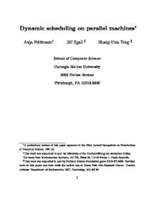
small support. While the first method tries to optimize the variable quantification scheme obtained for the subsequent products, the second one tries to optimize the size of the current intermediate product. We prefer the second choice, whereas [1] selects the first one. Moreover, and most important we insert the ordering heuristic inside a dynamic procedure (see Section 7 for the complete pseudo-code and more details). As the heuristic presented in [1], our procedure has a quadratic cost, i.e., if n is the number of latch relations/clusters its complexity is O(n2 ). In principle we 4 Ordering the Latch Relations run it after each intermediate conjunction. In practice, to avoid too much overhead, at each application we compare the ordering We derive our ordering algorithm directly from [1] keeping into with the old one, and we end re-evaluating it as soon as it is stable consideration the analysis done in [8, 9]. In [9] the authors try to solve the following problem: Given a Boolean function f (x1 ; : : : ; xn ) enough. Experimentally we discover that the cluster order usually changes a lot during the first two or three image computations, and the BDDs for each of the input functions xi , how should the and after that point it remains relatively stable. BDD for f be constructed so that the intermediate memory required to build the BDD is minimized? The authors present a set 5 Clustering the Latch Relations of heuristics (minimum-size-first, minimum-support-first, minimumextra-support-first, etc.) based on the support of the function, as As described in Section 3 clustering is usually a linear process well as their size (in terms of BDD nodes). They also present a based on a BDD size threshold. Moreover, clustering is usually heuristic based on a partial traversal of the BDDs, i.e., a partial done once and for-all at the beginning of the traversal process. pre-computation of the operation before the final computation to We propose an on-the-fly clustering done after an initial phase decide which possible operation is the best one. of traversal with the purpose of minimizing intermediate peaks in We start from these considerations trying to keep into account terms if the size of the BDDs involved in the computation. Our the strong impact of early quantification that usually drastically process is based on the following considerations. In [11] the auhelps in simplifying intermediate products. First of all, we try thors show that very often traversal processes require the maxito apply a try-and-abort heuristic: We select the best candidates mum number of BDD nodes during intermediate traversal levels. among a set of good ones by partially computing the conjunction. This consideration usually holds also inside intermediate evaluaThis methodology did not perform particularly well especially in tion of the image computation. As a consequence let us suppose terms of CPU time. As a consequence we propose the followto have a situation like the one represented in Figure 1(a), indeed ing algorithm taking into consideration five factors. We refer to a very common situation. It plots the BDD size of each intermeSection 3 for some of the definitions used here. Then we define:
Wi
=
qjj jjcjj jjejj � jjqjjmax jj + w2 � jjcmax jj + w3 � (1 jjemax jj )+ jtj jjxjj w4 � (1 jjxmax jj ) + w5 � (1 jtmax j ) w1
We select the term with the highest Wi value as next term to conjoin with P. Again, following [1], w1 ; : : : ; w5 are generic weights, but we are more drastic to characterize the weight of each factor as we select w1 = 10; w2 = 1; w3 = 1; w4 = 1; w5 = 2, giving higher priority to the quantification scheme and to the size of the BDDs involved. Notice that some of the introduced terms are similar to the ones presented in [1] but not equivalent. In particular we consider the size of the terms, not only their support. Moreover, we propose a different strategy regarding the support of the function. To this regard, two strategies are possible: Giving priority to function with a large support or giving priority to a function with a
|BDD|
3
m
step
{
step 1 2
{
n
{ {
12
{
Using the subscript max to indicate the maximum of the value among all the latch transitions still to be conjoined with P, we evaluate the following cost function for all the t term still to be conjoined:
|BDD|
{
� c = variables common to t and P � e = (extra) variables in t but not in P � jtj = size of t in terms of BDD nodes.
clusters
(a)
(b)
Figure 1: BDD Peaks during Image Computation. diate product as a function of the number of steps performed, i.e., the number of conjunction already computed. Our idea is to ideally start with no clustering at all (i.e., with n latch relations), and proceed with a self-tuning process that tries to smooth the curve of Figure 1(a) avoiding intermediate peaks. A possible solution is the one reported in Figure 1(b) where clusters are formed starting from the latch relations whose conjunction produces the peak BDDs. More formally the algorithm works as follow. During each image computation, we collect information about the size of intermediate products. Then, at clustering time, we evaluate the maximum values obtained. Each latch relation producing a peak size BDD is conjoined with one of its neighbor terms. During conjunction, we also use a size threshold to avoid memory blow-
up. We conjoin a term if its size is smaller than the threshold and we keep the result only if it is smaller than two times the threshold. We usually perform different steps of clustering, using peak size information coming from different traversal levels, to cluster the terms enough. We experimentally evaluate that a good heuristic consists in starting from a relatively small cluster size threshold and double it after each successive clustering.
6 Partitioning We follow [10] to mix the usual conjunction of terms with recursive case splitting. Our purpose is to simplify a costly operation op between two BDDs a and b, resorting to the well known “divide–and-conquer” strategy (a1 + a2 ) op b = (a1 op b) + (a2 op b) where a1 and a2 can be recursively partitioned. Decomposition is done by selecting a splitting variable v , that induces a partitioning also on the b operand: a op b = (av op bv ) + (av� op bv� ). We use this mechanism embedded in a recursive image computation procedure. The method uses two user-defined thresholds. The first one is a BDD size: We partition each single intermediate term whenever its size exceeds the threshold. The second one is a limit in the number of recursions for partitioning, i.e., we limit the number of partitions performed recursively. Experimentally we discover that this strategy gives better results and limits partitioning overheads.
7 Implementation and Pseudo-Code The ideas presented so far are implemented and better detailed in the following set of algorithms. T RAVERSAL (T , �) � New From � Reached �
level
1
6 ; 2
while (New = ) do if (level [CLUSTER F ROM, CLUSTERT O]) then C LUSTER DYNAMICALLY (T , size, ord) I MG (T , From, size, ord, 0, PART D) To To Reached New Reached + New Reached B EST BDD (New, Reached) From
�
level
level + 1
return (Reached)
Figure 2: Symbolic Forward Traversal. Figure 2 represents the top-level pseudo-code, i.e., a standard breadth-first traversal routine with our modifications. The T parameter is the initial set of n latch relations ideally with no clustering. Notice moreover that some initial clustering is possible in the case of models with a very large number of latches or with particularly small BDDs representing them. In this case we apply our ordering heuristic and a size threshold based clustering mechanism. Our first modification to the standard function is the presence of the function C LUSTER DYNAMICALLY. It clusters T trying to minimize the BDD peaks obtained during the previous image computation. It follows the strategy illustrated in Section 5. To avoid useless overheads it is called only when necessary, i.e,
during intermediate traversal levels (from the CLUSTER F ROM to the CLUSTERT O level), avoiding easy level and till we have obtained a satisfactory clustering. C LUSTER DYNAMICALLY (T , size, ord) eliminate duplicate values into array size for each i such that sizeordi 1 sizeordi if ( tordi CLUSTERT H ) then r = tordi tordi+1 if ( r < 2 CLUSTERT H) then extract tordi and tordi+1 from T insert r in T modify array size accordingly
j
j�
jj
�
� sizeordi+1 do
� �
Figure 3: Dynamically Cluster T . Function C LUSTER DYNAMICALLY is described in Figure 3. The ti terms are clustered around the ones that gave the higher BDD peaks during the previous image computation. size is the array used, by function I MG, to store the BDD size after each intermediate conjunction. ord is the array assigned by function S ELECT B EST C LUSTER (see Figure 5) to indicate the order of the clusters used to evaluate the image. During clustering the size of the new clusters is checked with a double threshold mechanism based on the CLUSTERT H value. I MG (T , Pi , size, ord, i, PART D) if (i number of ti in T ) then return (Pi ) ordi = S ELECT B EST C LUSTER (T , Pi , i) f tordi Pi+1 x (Pi f ) sizei Pi if ( Pi+1 < PART T H OR PART D < 0) then r I MG (T , Pi+1 , size, ord, i + 1, PART D) else var VAR S ELECT (Pi+1 ) t I MG (T , Pi+1 var , size, ord, i + 1, PART D 1) e I MG (T , Pi+1 var, size, ord, i + 1, PART D 1) r t+e return (r )
�
j
9 � j j j
� �
Figure 4: Image computation with Dynamic Ordering and Clustering, and Disjunctive Partitioning. Our second set of modifications is embedded into function I MG, detailed in Figure 4. It introduces our image computation routine. Whereas the standard formulation is linear, our procedure is recursive and it includes disjunctive partitioning of large terms. We indicate with i the number of conjunction performed during the current image computation, and with PART D the partitioning depth, i.e., the number of recursive partitioning still allowed. It essentially computes Pi+1 = x (Pi tordi ), where Pi is the current partial product and tordi is the element of T in position ordi . ordi is set by function S ELECT B EST C LUSTER (see Figure 5). If Pi has a BDD whose size is smaller than the threshold PART T H or the maximum level of recursions in term of partitioning has already been reached, the procedure recurs. Otherwise it partitions this partial product Pi and the recurs in a similar way on the two partitions. The BDD Pi is partitioned by computing a splitting variable by function VAR S ELECT . This function was
9
�
firstly described in [10], but various implementations of similar functions can be directly found in [13]. It basically selects the best variable in the set of support of Pi to cofactor Pi itself so to obtain the two smallest cofactors possible. Notice that as a single partitioning temporarily increases the number of BDD nodes, a certain care has to be paid during this phase to avoid unnecessary memory blow-ups. S ELECT B EST C LUSTER (T , P, i) i TO m for j compute qordj , cordj , eordj , xordj , tordj update qmax , cmax , emax , xmax , tmax for j i TO m qord cord eord Wj = w1 qmaxj + w2 cmaxj + w3 (1 emaxj )+ jtord j xord w4 (1 xmaxj ) + w5 (1 jtmaxj j ) return (j such that Wj is maximum)
j
� �
�
�
j
j
j
�
Figure 5: Recursive Relational Product with Disjunctive Partitioning. Figure 5 shows the procedure used to compute statistics and evaluate the order for latch/cluster relations. It computes the weight Wi as described in Section 4 and then uses these weights to evaluate the order ord of the clusters.
8 Experimental Results The presented technique is implemented within a traversal program built on top of the Colorado University Decision Diagram (CUDD) package [13]. Our experiments ran on a 550 MHz Pentium II Workstation with a 256 MByte main memory, running RedHat Linux 7.1. We present data on a few ISCAS’89 and ISCAS’89–addendum benchmarks, selected with different sizes, within the range of circuits manageable by state–of–the–art reachability techniques. 8.1 Case Study: s1269 In this section we present detailed data and a complete comparison for circuit s1269. Albeit its transition relation and its reachable state set are relatively small, the third level is extremely complex to traverse, with a very high peak in terms of BDD nodes. This characteristic is mainly due to a bad behavior of all known heuristics to deal with that model during image computations, and makes it extremely suitable for extensive analysis. In Table 1 our methodology is compared with the one presented in [1] and data taken from the literature [3, 4, 5]. For rows [1] all the data are obtained with our implementation of the original algorithm. On the contrary, rows [4]-[1] show results obtained with the same methodology implemented in VIS [14] and derived by [4]. As introduced in Section 3 minor implementation differences may give different results, and this consideration may explain the different data reported in the table. All the other data are extracted from the referenced papers. In all the cases standard breadth–first traversal is considered. We are aware that better results may have been presented with some other technique, i.e., guided traversal, but we consider this work as orthogonal as all kinds of reachability analysis (guided, over-approximate, underapproximate, etc.) may take advantages from any improvement in the underlying image computation procedure.
In the top part of the table, we start the experiment with a statically computed variable order (obtained with a standard depth first search performed on the original source BLIF file, see [14] for example). These experiments show results in a common experimental environment, where dynamic variable reordering is automatically activated whenever necessary. This part of the table is divided into three more sections. In the first/top one, we compare our methodology with [1] without clustering: This allows us to compare ordering heuristics as a solo heuristic, i.e., without any sort of clustering involved. In the second/middle one, we compare a few cases of usual traversal, including ordering and clustering. In the third/bottom one, we compare strategies involving some sort of partitioning. In the bottom part of the table, we start our traversal from an already optimized BDD variable ordering (obtained from [10, 15]) and with dynamic variable reordering disabled. These experiments show the performance and contributions of the various algorithms without the influence of dynamic variable reordering. This may be useful because albeit being really beneficial dynamic variable reordering is a large source of noise and may randomly modify performances. The meaning of the columns follows the terminology used in Section 7: CLUSTERT H indicates the threshold (in terms of number of BDD nodes) used to cluster T , PART T H is the threshold used to disjunctively partition intermediate products, Peak Live Nodes is the peak of BDD nodes during the process, Peak Size is the size of the larger BDD created during the process. Finally, Mem. and Time indicate respectively memory occupation (in MBytes) and CPU time (in seconds). As a final remark notice that a direct comparison of all the data (e.g., time values) should give a rough idea of performance but may be unfair. In fact, initial variable orders are not always comparable and experiments are performed on different hardware configuration, as reported at the end of the table. To conclude, let us notice that our heuristic usually performs pretty well especially in terms of memory. As far as CPU time is concerned, we pay two sources of overheads: (1) The heuristic is intrinsically more expensive than the original one; (2) Some implementation inefficiency that would be avoided with a more accurate implementation. In any case, the overheads introduced to are often more than balanced by the saving obtained in terms of BDD nodes and CPU time as a direct consequence. 8.2 Other Experiments We follow is this section the flow used in the previous one. First of all, we present some data showing the impact of dynamically reordering the terms ti , without clustering them. In Figure 6 we compare, on three circuits, our dynamic ordering methodology with the one in [1] without clustering, i.e., the clustering threshold was set to zero. We plot the peak live nodes used as a function of the traversal level. In all the cases we report only meaningful traversal iterations. Again in this case we use an initial optimized variable order and dynamic variable order is disabled, to better isolate the experiments from the noise introduced by dynamic variable reordering. In Table 2 we compare our methodology with our implementation of the one presented in [1] on a set of benchmark circuits. To set-up this table we use the same strategy used for Table 1.
Method
CLUSTERT H
PART T H
Peak Live Nodes
Peak Size
Mem. [MByte]
Static Initial Variable Order - Dynamic Variable Reordering Enabled [1] 0 0 6819019 5130600 186 This Paper 0 0 1420778 759356 53 [1] 5000 0 1498205 1008719 52 [4]–[1] 0 3652300 [4] 0 1413900 [5] 600000 46 This Paper 2000,4000 0 794034 480942 36 [3] 1576000 This Paper 2000,4000 100000,3 643710 296151 30 Optimized Initial Variable Order - Dynamic Variable Reordering Disabled [1] 0 0 7632364 3874167 161 This Paper 0 0 1519305 859208 51 [1] 500 0 4136867 2921359 97 [1] 5000 0 1654485 1189487 56 [4]–[1] 0 9000000 [4] 0 25565000 This Paper 2500 0 1235446 652473 47 This Paper 2500,5000 0 1234138 652473 46 This Paper 2500 100000,3 836881 422826 37 Reference This Paper, [1] [3] [4] [5]
Time [sec] 8979 1123 985 6429 1658 1877 892 891 653 365 246 230 242 178 283 154 160 316
Machine Pentium III, 550 MHz, 256 MByte Pentium II, 400 MHz, 1 GByte Pentium II, 400 MHz, 750 MByte UltraSPARC Workstation, 296 MHz, 768 MByte
Table 1: Reachability Analysis Comparison for circuit s1269. Optimized variable ordering are taken from [16, 15]. Circuit s3271 is the one on which our ordering and clustering heuristics obtains the worst results, as the memory reduction is mainly due to the partitioning methodology. In all the other examples the results are similar to the ones previously presented, with gains due both to a better ordering and a better clustering with some further reductions due to partitioning.
9 Conclusions The core computation in both synthesis and verification is forming the image and pre-image of sets of states under the transition relation characterizing the design. Existing algorithms are mainly limited by memory resources in practice. To make them as efficient as possible, we address a set of heuristics with the main target of minimizing memory usage. These include an heuristic to order the latch relations, a new framework to cluster them and the application of conjunctive partitioning during the computation. We provide and integrate a set of algorithms and we give reference and comparison with recent work. Experiments are given to demonstrate the efficiency and robustness of the approach.
References [1] R. K. Ranjan, A. Aziz, R. K. Brayton, B. Plessier, and C. Pixley. Efficient BDD Algorithms for FSM Synthesis and Verification. In Proc. Int’l Workshop on Logic Synthesis, Lake Tahoe, California, May 1995.
means data not available.
[2] R. Hojati, S. C. Krishnan, and R. K. Brayton. Early Quantification and Partitioned Transition Relation. In Proc. Int’l Conf. on Computer Design, pages 12–19, Austin, Texas, October 1996. [3] I. H. Moon, J. H. Kukula, K. Ravi, and F. Somenzi. To split or to conjoin: The question in image computation. In Proc. 37th Design Automat. Conf., Los Angeles, California, June 2000. [4] I. H. Moon and F. Somenzi. Border-Block Triangular Form and Conjunction Schedule in Image Conjunction. In Proc. Formal Methods in Computer-Aided Design, volume 1954, Austin, TX, USA, 2000. Springer-Verlag. [5] A. Gupta, Z. Yang, P. Ashar, and A. Gupta. SAT–Based Image Computation with Application in Reachability Analysis. In Proc. Formal Methods in Computer-Aided Design, volume 1954 of LNCS, Austin, TX, USA, 2000. [6] C. Meinel and C. Stangier. Speeding Up Image Computation by Using RTL Information. In Proc. Formal Methods in Computer-Aided Design, volume 1954, Austin, TX, USA, 2000. Springer-Verlag. [7] C. Meinel and C. Stangier. Hierarchical Image Computation with Dynamic Conjunction Scheduling. In Proc. Int’l Conf. on Computer Design, Austin, TX, USA, 2001.
[1] This Paper 7e+06
6e+06
5e+06
9e+06
Peak Size BDD
Peak Size BDD
Peak Size BDD
8e+06
[1] This Paper 8e+06 7e+06 6e+06
1e+06 [1] This Paper 900000 800000 700000 600000
5e+06 4e+06
500000 4e+06 400000
3e+06 3e+06
300000 2e+06
2e+06
1e+06
200000
1e+06
0
100000
0 1
2
3
4
5
6
7
8
9
10
0 1
1.5
2
2.5
Traversal Level
3
3.5
4
4.5
5
1
1.5
2
2.5
Traversal Level
(Circuit s1269)
3
3.5
4
Traversal Level
(Circuit s4863)
(Circuit s5378179 )
Figure 6: Peak size BDD nodes without clustering.
Circuit
Level
[1] Peak Live Nodes
s1269 s3330 s4863 s5378121 s5378179
s1269 s3271 s3330 s4863 s5378121 s5378164 s5378179
Mem. [MByte]
Time [sec]
This Paper Peak Live Nodes Mem. [MByte]
Static Initial Variable Order - Dynamic Variable Reordering Enabled 9 1498205 52 985 643710 8 3526922 98 12290 2346778 4 493936 44 686 356798 42 225000 22 1658 123384 7 6986688 178 32939 3567896 43 ovf ovf ovf 6987977
Time [sec]
30 62 37 21 99 211
653 8970 674 946 27906 87696
Optimized Initial Variable Order - Dynamic Variable Reordering Disabled 9 1654485 56 242 836881 37 16 1961389 54 458 1561389 50 8 3323454 86 10598 2235678 69 4 147034 21 17 139098 20 42 103898 20 308 81830 20 7 5029185 130 30112 1031218 30 43 ovf ovf ovf 3863728 114 43 2445189 71 23890 1769090 64
316 679 8647 29 340 5562 62002 18960
Table 2: Reachability Analysis Comparison.
means data not available. ovf means overflow on memory.
[8] R. Drechsler, A. Hett, and B. Becker. Symbolic Simulation using Decision Diagrams. Electronic Letters, 33(8):665– 667, 1997. [9] R. Murgai, J. Jain, and M. Fujita. Efficient Scheduling Techniques for ROBDD Construction. In Proc. VLSI Systems Design, India, 1999. [10] G. Cabodi, P. Camurati, and S. Quer. Improved Reachability Analysis of Large Finite State Machine. In Proc. Int’l Conf. on Computer-Aided Design, pages 354–360, San Jose, California, November 1996. [11] K. Ravi and F. Somenzi. High–Density Reachability Analysis. In Proc. Int’l Conf. on Computer-Aided Design, pages 154–158, San Jose, California, November 1995. [12] G. Cabodi, P. Camurati, and S. Quer. Improving Symbolic Traversal by means of Activity Profiles. In Proc. 36th Design Automat. Conf., pages 306–311, June 1999. [13] F. Somenzi. CUDD: CU Decision Diagram Package – Release 2.3.0. Technical report, Dept. of Electrical and Com-
puter Engineering, University of Colorado, Boulder, Colorado, October 1998. [14] R. K. Brayton et al. VIS. In Mandayam Srivas and Albert Camilleri, editors, Proc. Formal Methods in ComputerAided Design, volume 1166 of LNCS, pages 248–256, Palo Alto, California, November 1996. Springer-Verlag. [15] http://www.polito.it/
�fcabodi,querg.
[16] G. Cabodi, P. Camurati, and S. Quer. Improving Symbolic Reachability Analisys by means of Activity Profiles. IEEE Transactions on CAD, 19(9):1065–1075, September 2000.