Dynamic Spatial Backoff in Fading Environments Zhongning Chen
Xue Yang
Nitin H. Vaidya
Redback Networks, an Ericsson Company
[email protected]
Intel Corporation
[email protected]
Univ. of Illinois at Urbana-Champaign
[email protected]
Abstract—We present a dynamic spatial backoff method to resolve channel contention in wireless ad-hoc networks. We argue that each node should adjust its receiver sensitivity level according to the mean channel gain of its particular transmitter-receiver link, in order to see the full benefit of spatial backoff and improve the throughput. We designed a distributed algorithm that adjusts each transmitter’s carrier sense threshold and transmission rate dynamically based on local information and limited receiver feedback, for wireless channels that have small-scale multipath fading. We evaluated the algorithm using different topologies, under various fading conditions. Results show that our algorithm is able to achieve aggregate throughput near or better than the maximum achievable by the static scheme, without a priori knowledge of the network topology or fading condition.
I. I NTRODUCTION Two fundamental aspects of wireless communication make wireless ad-hoc networks different from wired networks. First, the channel gains of wireless stations vary over time due to the small-scale effect of multipath fading. Second, there is significant interference among wireless stations that are spatially close to each other since they share the same medium. Each transmission in the wireless network occupies a certain space. Intuitively, a Node B is said to be within the space occupied by a transmission from Node A, if a concurrent transmission from Node B will prevent reliable reception of A’s transmission. For example, in Figure 1(a), we depict spaces occupied by node A and B’s transmissions as circles around them (for the purpose of illustration only); A and B may not transmit concurrently on the same channel since they are within each other’s space. On the other hand, in Figure 1(b), A and B are outside of each other’s space and they can transmit concurrently without interfering with each other.
A
B
A
(a) Spatially overlapped
Fig. 1.
B
(b) Spatially separated
Different Spatial Separation
This research is supported in part by US Army Research Office grant W911NF-05-1-0246. Any opinions, findings, and conclusions or recommendations expressed in this paper are those of the authors and do not necessarily reflect the views of the funding agencies.
c 1-4244-2575-4/08/$20.00 °2008 IEEE
Past research on contention-based medium access control (MAC) protocols usually focused on temporal approaches. That is, when two nodes are competing for the same channel, their accesses to the channel are separated in time to ensure successful transmissions. In our example in Figure 1(a), since nodes A and B are not spatially separated, their transmissions have to be separated in time using temporal contention resolution. Such temporal approaches typically address the problem by adapting each node’s channel access probability to accommodate the given network’s channel contention requirement. Yang et al. [1]–[3] studied an alternative contention resolution approach for wireless networks, first introduced in [2] as spatial backoff, which adapts the space occupied by transmissions so that channel contention may be resolved more efficiently in both spatial and temporal dimensions. Usually, the space is in part dependent on the transmission power used, data rate of transmission, and carrier sense (CS) threshold of stations. MAC protocols play an important role in determining the three aforementioned parameters, and hence the spatial utilization. One popular scheme that is used in most wireless LANs is Carrier Sense Multiple Access (CSMA), in which each station senses the medium before it attempts to transmit. If the signal level detected at a station is below a CS threshold, the channel is decided to be idle, and the station may access the medium. Assuming a fixed transmission power is used by every station in the network, a node will transmit more aggressively using higher CS thresholds. For example, in Figure 1(b), concurrent transmissions from nodes A and B can be achieved by using large CS thresholds for both nodes. On the other hand, notice that the more concurrent transmissions (i.e., the higher the CS thresholds used at the transmitters), the higher the interference at the receivers, and therefore the lower the signal-to-interference-and-noise ratio (SINR), and consequently the lower transmission rates the packets can be transmitted reliably. In contrast, the fewer the concurrent transmissions, the higher the SINR at the receivers, and the higher transmission rates the packets can be transmitted reliably. In other words, the space occupied by a transmission is jointly determined by the transmission rate and CS threshold. Therefore, in order to achieve a high aggregate throughput in a network, there exists a trade-off between CS threshold and transmission rate at each transmitter.1 1 One may also choose to vary transmission power to realize spatial backoff [6]. However, power control creates asymmetric links and has further complications. The joint adaptation of the 3 parameters, transmission power, rate, and CS threshold, may have benefits [17], which is an on-going work.
A spatial backoff algorithm has been proposed by Yang et al. [1] [3] to approach the optimal trade-off between CS thresholds and transmission rates to achieve high aggregate throughput in an ad-hoc network. However, our study has found that its performance suffers in the presence of smallscale multipath fading. This paper proposes a modified dynamic spatial backoff algorithm that can resolve channel contention using spatial backoff and achieve a high level of aggregate throughput in ad-hoc networks, even with channel and traffic variations over time. In the rest of the paper, we refer to the algorithm by Yang et al. [1] [3] as ODSB, and our proposed algorithm as dynamic spatial backoff. The rest of the paper is organized as follows. Section II summarizes the related work. Section III explains the importance of setting the appropriate receiver sensitivity. Section IV describes the dynamic spatial backoff algorithm, which is evaluated in Section V. Section VI concludes the paper. II. R ELATED W ORK Studies on medium access control to address the channel contention had been conducted extensively in the time domain. Temporal contention resolution typically takes the set of competing stations as given, and addresses the issue of how to separate transmissions from competing stations in time to achieve successful transmissions. Numerous methods have been proposed to achieve the temporal separation of transmissions while reducing the overhead introduced by medium access control. Examples of such proposals include [4]–[6]. Physical carrier sensing, transmission power control, and transmission rate control provide effective ways to control the interference and the amount of spatial reuse in the network. Guo et al. [7] and Zhai et al. [8] noted the impact of CS threshold on the aggregate throughput. Assuming that the transmission rate is fixed for a given network, Zhu et al. [9], [10] proposed algorithms that dynamically adjust the CS threshold to improve spatial reuse and aggregate throughput; [9] also used the receiver sensitivity as a parameter in their adaption algorithm design. Other works that aim to improve spatial reuse by adjusting CS threshold include [11] by Vasan et al. and [12] by Nadeem et al. The common limitation of the above works is that a fixed transmission rate is assumed. With a fixed transmission rate, CS threshold adaptation algorithms can only find CS threshold suitable to this particular rate. However, by reducing the transmission rate and using a higher CS threshold, one may be able to further improve the spatial reuse and the local channel contention resolution efficiency. CS threshold adaptation algorithms alone cannot exploit such benefits. There also exist some rate control algorithms such as [13] and [14], which aim at adapting the transmission rate based on channel conditions. The problem with the rate control algorithms is that they primarily only adapt to the change of the quality of the wireless link, and do not address the channel contention problem. Therefore, in a dense network where many nodes compete for channel access, rate control alone will not work well.
Prior work has also proposed to use power control protocols to improve spatial reuse, by introducing new transmissions without interrupting existing transmissions [15], [16]. Fuemmeler et al. [17] and Mhatre et al. [18] have explored the joint control of transmission power and CS threshold to reduce collisions. Existing work such as [19], [20], on topology control has addressed the issues of finding the appropriate transmission power each node should use. The objective is to maintain network connectivity while reducing energy consumption and improving network capacity. Finally, without taking fading into account, Kim et al. [21] proposed an algorithm that jointly controls transmission power and rate to improve spatial reuse. III. D ETERMINING R ECEIVER S ENSITIVITY Let RXth denote the receiver sensitivity, or the smallest power level of the received signal required for correctly decoding at the receiver. IEEE 802.11a defines the minimal receiver sensitivity for different data rates, as listed in Table I [22]. TABLE I R ECEIVER SENSITIVITY FOR DIFFERENT DATA RATES Data Rate (Mbps) 6 9 12 18 24 36 48 54
Receiver Sensitivity (dBm) -82 -81 -79 -77 -74 -70 -66 -65
The capture effect is the ability of a radio to correctly receive a signal from one transmitter despite interference from another transmitter, if the received SINR is above a certain capture threshold. In an 802.11 ad-hoc network, a receiver A can be triggered by an interference signal even if A is not the intended receiver of the signal. Furthermore, most of today’s 802.11 radios will not capture a stronger signal that arrives later while it is locked onto the first signal, even if the later is the intended signal and is strong enough. Hence the later packet will be lost by A. Moreover, the transmission of the later packet still causes enough interference to disrupt the on-going reception of the first packet. As a result, both packets are lost. This type of collision is called a strongerlast collision [23]. Similar situation can occur at a transmitter as well. A transmitter can be triggered by an interference signal, and falsely lock into receiving mode until the entire incoming packet is finished receiving. In the meantime any outgoing traffic has to defer until the falsely triggered reception is completed. Intuitively, if the receiving mode can be less easily triggered, throughput can be increased and delays can be decreased in 802.11 networks. It was first proposed in [9] to adjust the RXth of each receiver in a WLAN to only receive the signals from the access point (AP) which has the strongest signals among all
APs. We extend this idea to ad-hoc networks. For a transmitterreceiver (Tx-Rx) link, let S˜ be the received signal strength at the receiver Rx (RSS) from the transmitter Tx averaged over time, and σ be the RXth adaptation safety margin, we have S˜ RXth = (1) σ or RXth (dBm) = S˜dBm − σdB for receiver Rx. The safety margin is needed because the RSS is not a constant in fading environment but is rather stochastically distributed. Note that ˜ which depends on the channel gain RXth is a function of S, of each particular transmitter-receiver (Tx-Rx) link. For example, in the single-hop scenario in Figure 2, Node B measures its RSS, or S˜ from Node A, and determines its RXth based on Equation 1. Similarly, Node A can measure its S˜ from Node B, either through training signals or ACKs from Node B, and then decides its appropriate RXth . A Fig. 2.
B
Adjustment of RXth in a single-hop scenario
IV. DYNAMIC S PATIAL BACKOFF A LGORITHM For a given transmission from some node Tx to another node Rx, for future reference, we define concurrent transmissions as other transmissions that can overlap in time with the Tx-Rx transmission without causing unreliable reception at Rx. We also define simultaneous transmissions as those transmissions from local contending nodes within the occupied space of the Tx-Rx transmission, which start shortly before or after the start of Tx-Rx transmission and cause erroneous reception at Rx (commonly known as collisions). Notice that carrier sensing cannot help prevent simultaneous transmissions that start within a short time interval, due to the delay required for carrier sensing, such as propagation delay; nor can it help prevent packet loss caused by channel variations. The goal of the proposed spatial backoff algorithm is to allow each node to dynamically adjust the CS threshold and the transmission rate to determine the suitable values of these two parameters at any given time, based on the current network and channel condition. We define an operating point as a combination of CS threshold and transmission rate. For simplicity, we often associate these two parameters with the source node, but they in fact correspond to each link. Ideally, we would like to find the optimal operating point for each flow such that the network aggregate throughput can be maximized. However, since aggregate throughput is a global metric, it is not always possible to find the optimal operating point to maximize the metric based only on local information available at the transmitter and receiver. As such, the goal of our work is to design a simple mechanism that can be easily incorporated into existing MAC protocols to take advantage of spatial backoff and to improve aggregate throughput. One of the challenges in our algorithm design is the smallscale fading effects. There are different types of fadings caused
by different propagation mechanisms. Here we focus on flat fading, where the amplitude of the received signal changes with time, due to fluctuations in the gain of the channel caused by multipath. From a transmitter point of view, when a packet is lost (i.e., an ACK is not received), it is not clear whether it is because of interference, or because of poor channel condition. Similarly, if a transmission succeeds (i.e., an ACK is received), it is also not obvious whether it is because the channel gain is high, or because the interference is low at that particular moment. To maximize the aggregate throughput, it is desirable to exploit the opportunistic gain by using higher transmission rate when the channel gain is on the rise. Therefore, we introduce a binary receiver feedback mechanism, in which an information bit B is piggy-backed in the ACK packet upon successful transmission. B is defined as follows: • B = 1, if the latest received packet’s SINR meets the SINR requirement of the next higher data rate level plus a margin θ associated with that rate. If the highest data rate is already in use, then B = 1 when the latest received packet’s SINR exceeds the SINR requirement of the highest rate plus the margin θ. • B = 0, if the latest received packet’s SINR does not meet the aforementioned conditions for B = 1. The use of B and determination of the RXth , as described in Section III, require the receiver to be able to measure its RSS and track its own channel SINR. Such features are already present in many 802.11 products. One example is the ORiN OCOr Classic Gold PC Card. The use of B in our algorithm will be presented in Section IV-B. A. Determine Operating Points The proposed dynamic algorithm allows each node to choose any combination of the two parameters, CS threshold and transmission rate, and adjust the combination based on the locally available channel information. While the number of levels of transmission rate is usually limited by the wireless device implementation, the possible levels of CS threshold, which is a continuous value lower bounded by the radio sensitivity, is potentially unlimited. A naive exhaustive search in the two-dimensional space defined by the CS threshold and transmission rate can lead to poor performance. Therefore, the design of our dynamic spatial backoff algorithm includes reducing the search space by limiting ourselves to a finite set of CS thresholds, and incorporating suitable search rules. We let each node determine its own set of carrier sense thresholds for different data rates. We consider an interference limited environment. For each channel rate, there is a required SINR if a certain bit error rate (BER) needs to be achieved. Table II shows the required SINR for BER less than or equal to 10−5 [24]. Suppose there are M available data rates. We represent them using an array Rate[], where Rate[i] < Rate[j] if i < j (i, j ∈ [1, . . . , M ]). If SIN R[i] is the SINR threshold for Rate[i] (i ∈ [1, . . . , M ]), on average, interference less than ˜ or equal to SINSR[i] shall not affect the correct reception at
TABLE II SINR REQUIREMENT FOR DIFFERENT DATA RATES
R index
SINR Requirement (dB) 6.02 7.78 9.03 10.79 17.04 18.80 24.05 24.56
Rate Fig. 3.
Rate[i], if the received power is more than S˜ on average. We let the transmitter estimate the interference at the receiver using its own perceived interference level and define CS[i], the carrier sense threshold for each data rate Rate[i], as follows: CS[i] =
S˜ SIN R[i]
(2)
B. Algorithm Description With M transmission rates available, we define rate level as a number from 1 to M such that rate level 1 is the lowest transmission rate Rate[1], and rate level M is the highest rate Rate[M ]. In addition to rate array Rate[] and CS threshold array CS[], each node also maintains an index variable Rindex and an index array CSindex []. Rindex represents the array index for Rate[] (i.e., transmission rate = Rate[Rindex ]), where Rindex ∈ [1, . . . , M ]. Given the Rindex , there is an associated CS threshold array index CSindex [Rindex ]. Both Rindex and CSindex [Rindex ] are dynamically adjusted. At any given time, a node will transmit at rate Rate[Rindex ] using the associated CS threshold CS[CSindex [Rindex ]]. The data structure is illustrated in Figure 3. At each node, Rindex is initialized to 1, and CSindex [i] is initialized to i, ∀i ∈ [1, . . . , M ]. Each node starts from using the transmission rate Rate[1] and the CS threshold CS[CSindex [1]] = CS[1] (i.e., the lowest rate and highest CS
CS
Data structure of dynamic spatial backoff
threshold). We define two additional arrays, S[] and F [], each of size M ; their elements are initialized to Smin and Fmin , respectively. They hold the number of desired consecutive successes and consecutive failures a node has had, respectively. A node will take different actions, depending on whether its past transmissions have been successes or f ailures, and the information bit B fed back from the receiver. The actions of each node are governed by the 5 rules below. Note that in the following text, “diagonal line” refers to the diagonal in Figure 4. Each rule described hereafter is depicted in Figure 4 with an arrow and the rule index right next to it. 2 Rate[M] 3 Rate[M−1] ...
Given the estimated interference, if the detected signal strength at the transmitter is no higher than CS[i], it can start transmitting at Rate[i]. The receiver will be able to correctly receive the signal with SINR no less than SIN R[i] in the absence of additional interference. On the other hand, if there is additional interference at the receiver side, the receiver may not be able to correctly receive the signal, as a result of inaccurate estimation of interference at the receiver. Our simulation results shown in later part of this paper indicates that this interference estimation works reasonably well in dense networks, which is the scenario where spatial backoff is most needed. If the network is sparse, the benefit of spatial backoff is limited because each node does not experience much interference in the first place. Similar to RXth , CS[i] defined in Eq. 2 is also a function of average channel gain and is different for different flows. Since the SINR threshold is higher for a higher rate, it follows that CS[i] > CS[j] if i < j (i, j ∈ [1, . . . , M ]) at a given node.
111111 000000 000000 111111 000000 111111 000000 111111 000000 111111
CS index
Increasing transmission rate
Data Rate (Mbps) 6 9 12 18 24 36 48 54
000000 111111 000000 111111 000000 111111 00000000 11111111 000000 111111 000000 111111 000000 111111 000000 111111
111111 000000 000000 111111 000000000000 111111 111111 000000 111111 000000 111111 000000 111111
Rate[3] 4
1 Rate[2]
5 Rate[1] CS[1]
CS[2]
CS[3] . . .
CS[M−1] CS[M]
Decreasing CS threshold
Fig. 4.
Search space for the dynamic spatial backoff algorithm
1) When there are S[i] (i ∈ [1, . . . , M ]) consecutive successes and the highest transmission rate is not in use: The node will increase its transmission rate by one level if the feedback bit B in the last received ACK equals 1 (i.e., Rindex := Rindex + 1), while keeping the CS threshold the same, i.e., using the new Rindex , CSindex [Rindex ] := CSindex [Rindex − 1]. Motivation for Rule 1: B = 1 in the very last received ACK indicates that the interference at the receiver is small enough, or the channel gain is large enough, so that SINR requirement for the next rate level is met. We do not require all S[i] consecutive ACKs to have B = 1 before the transmission rate is increased, so that in the case when the channel is varying fast, we can quickly catch the rise of the channel gain to use the higher transmission rates. We keep the CS threshold at the same level so that the transmitter can take advantage of the good channel condition without becoming more aggressive for its neighbors.
2) When there are S[i] consecutive successes and the highest transmission rate is already in use (i.e., Rindex = M ): If the highest CS threshold is not already in use (i.e., CSindex [Rindex ] > 1), the node will increase its CS threshold by one level if the feedback bit B in the last received ACK equals 1, while keeping the same transmission rate. In other words, CSindex [Rindex ] := CSindex [Rindex ] − 1. Motivation for Rule 2: Recall that CS[j] > CS[i] if j < i (i, j ∈ [1, . . . , M ]). As defined in the beginning of this Section, in the case when the highest transmission rate is already in use, B = 1 indicates that the SINR at the receiver exceeds the SINR requirement for the highest transmission rate plus an associated margin θ. This tells us that the channel is currently very good and there is still remaining interference tolerance margin at the receiver. Therefore we exploit this margin by increasing the CS threshold. 3) When there are F[i] consecutive failures and the operating point is strictly above the diagonal line (i.e., Rindex > CSindex [Rindex ]): The station will decrease its CS threshold by one level (i.e., CSindex [Rindex ] := CSindex [Rindex ] + 1), while the transmission rate will remain the same. Motivation for Rule 3: The derivation of CS[i] in Eq. 2 tell us that, when the operating point is strictly above the diagonal line, the reason why transmissions fail is likely because the transmitter has overestimated the interference tolerance margin at the receiver (either because there is too much interference or because the received signals are too weak). To increase the likelihood of successes at the current transmission rate, we reduce the CS threshold at the transmitter, which will help it to transmit more conservatively. 4) When there are F[i] consecutive failures and the operating point is on or below the diagonal line and the lowest transmission rate is not already in use (i.e., Rindex ≤ CSindex [Rindex ] AND Rindex > 1): The station will decrease its transmission rate by one level (i.e., Rindex = Rindex − 1) and the CS threshold associated with the lower transmission rate will be used. Motivation for Rule 4: When we define CS[i] for each Rate[i] (i ∈ [1, . . . , M ]), we mentioned that it is expected that using CS[i], a station will transmit successfully at rate Rate[i]. Therefore, if the station fails at rate Rate[i] when using a CS threshold value lower than or equal to CS[i], it is very likely that the surrounding interference is too high or the channel is too bad to support the current transmission rate. By reducing the transmission rate, more interference or poor channel can be tolerated at the receiver. Moreover, our data structure helps the station to remember the last CS threshold used when transmissions were successful at the lower rate. Therefore, the station is likely to transmit successfully at the new rate.
5) When there are F[i] consecutive failures and the lowest transmission rate is already in use (i.e., Rindex = 1): The station will decrease its CS threshold by one level (i.e., CSindex [Rindex ] := CSindex [Rindex ] + 1) unless the lowest CS threshold is already in use. Motivation for Rule 5: There are two possible reasons for transmissions to fail at the lowest rate: (A) the interference at the receiver is too high, or (B) the channel fades. Both result in the SINR requirement for the lowest rate not being satisfied. In such cases, the station can attempt to improve the situation by transmitting more conservatively through lowering the CS threshold. Notice that in a fading environment, with small but nonzero probability, the channel will go into a fading state that is too deep for the transmitter to successfully send anything. When this happens, following the rules above, the operating point may end up at a low CS threshold using the lowest rate. After the channel gets out of the deep fade state, the station will start transmitting successfully again. However, now it may be using a CS threshold smaller than necessary (i.e., too conservative). We used the following deterministic Special Rule to prevent the CS threhsold from sticking to a low value: If an operating point is below the diagonal line (i.e., Rindex < CSindex [Rindex ]), the station marks this operating point once when S[i] consecutive successes are achieved (regardless of the B value). Each operating point below the diagonal line has an associated marking number. If the number of markings for this operating point exceeds some threshold, say Imax , instead of following the Rule 1 mentioned above, we increase CS threshold by one level (i.e., CSindex [Rindex ] = CSindex [Rindex ] − 1), while keeping the transmission rate at the same level. The marking number of that operating point will then be reset to 0. This way the station gets a chance to probe a different combination of CS threshold and transmission rate to exploit the remaining channel capacity. Heuristically, we let Imax = 2 in our design. To illustrate how a transmitter adapts to contention and change of channel condition due to small-scale fading, we plotted a typical operating point trajectory of a transmitter in Figure 5. The horizontal axis of Figure 5 represents the CS threshold value and the vertical axis represents the rate. Here we assume there are four rate levels, i.e., M = 4. The rule applied to each movement is labeled right next to each arrow. In this scenario, the link quality was good enough to support Rate[3], so the transmitter advanced its operating point to (CS[1], Rate[3]) by applying Rule1. It then failed on an attempt to increase the transmission rate to the next level (i.e., Rate[4]), probably due to collisions or bad channel quality. So it kept decreasing its CS threshold by applying Rule3 until the smallest CS threshold was reached. When successive failures occurred at that operating point, it applied Rule4 and went back to the previously successful operating point at the next lower rate, which is (CS[1], Rate[3]). To avoid performance loss due to frequent unsuccessful
(3) (1)
(3)
(3)
(4)
Rate[3] (1)
Rate[2] (1)
Rate[1] CS[1] CS[2] CS[3] CS[4]
Decreasing CS Threshold
Fig. 5. Operating point movement in the dynamic spatial backoff algorithm
probing, the values of S[] and F [] are adjusted dynamically. Intuitively, if a node can transmit at the rate level Rindex with high success rate, but it fails often at the rate level Rindex + 1, we would like the node to probe the rate level Rindex + 1 less frequently. Therefore, we utilized a concept mentioned in [25] to guide the adjustment of S[] and F []. In [25], the authors presented an idea to use Loss Estimation to do rate change. The basic idea is as follows. At a particular transmission rate, if the packet loss ratio in an estimation window (defined by number of packets) is so high that it exceeds some threshold, say PH , that using the next lower transmission rate will give a higher throughput (assuming 100% success rate at the next lower transmission rate), then the transmitter will lower its transmission rate. On the other hand, if the packet loss ratio is so low that it is smaller than some threshold, say PL , and using the next higher transmission rate will likely give higher throughput, even with some amount of packet losses, then the transmitter will increase its transmission rate. We utilized the concept of loss ratio to guide the adjustment of S[] and F []. If the packet loss ratio at transmission rate Rate[i] (i ∈ [2, 3, . . . , M ]) in a fixed estimation window2 is lower than PL [i], there is no point in decreasing the transmission rate, because even if transmissions at the next lower rate have 100% success rate, it will not likely give a higher throughput. In this case, we adjust F [i] to F [i]+1. Conversely, if the packet loss ratio at that transmission rate is higher than PH [i], then we adjust F [i] to max{F [i] − 1, Fmin }. Similarly, if the packet loss ratio at rate Rate[i] is higher than PH [i], the station should not probe an even higher transmission rate because it will probably experience even higher packet loss; hence we increase S[i] to S[i] + 1. On the other hand, if the same packet loss ratio drops to below PL [i], the station should probe the higher transmission rate more often because it may give a higher throughput. Therefore, we decrease S[i] to max{S[i] − 1, Smin }. In our current design, Smin = 3, Fmin = 2, and estimation window = 40 packets. V. E VALUATION R ESULTS AND D ISCUSSIONS A. Simulation Setup We simulated the proposed dynamic spatial backoff algorithm using a modified Network Simulator 2 (ns-2) version 2 Ideally, the estimation window size should be a function of the speed of channel variation.
2.26. Each node’s transmission power was fixed at 100 mW. Each transmitter has four available data rates: 9 Mbps, 18 Mbps, 36 Mbps, and 54 Mbps. We used UDP traffic and each packet’s payload size was fixed at 512 bytes. Rician fading model was used to model the flat fading environment, in which the nodes were fixed but there were movements of objects around them. We varied the Rician K factor and the vmax to simulate different Rician fading scenarios. Here vmax is the maximum velocity at which the sorrounding objects move, or vmax = fm × λ, where fm is the maximum Doppler shift, and λ is the carrier wavelength. Rician K is defined as the ratio between the mean power of the line-of-sight (LOS) component in the channel, and the mean power of the scattering components. 1) Rician fading simulator: We used the Rician fading model described in [26]. We modified the implementation such that each link has independent, symmetric Rician fading. The effect of varying vmax is shown in the Figure 6, where the horizontal axis is time and the vertical axis is the fading envelope. The dotted curve is for vmax = 2.5 m/s, and the solid curve is for vmax = 0.5 m/s. The higher the vmax , the faster the Rician fading envelope varies, and thus the faster the received signal amplitude will vary. 2.5 2.5 m/s 0.5 m/s
2
Rician Envelope
Increasing Tx Rate
Rate[4]
1.5
1
0.5
0
0
1
2
3
4
5
6
7
8
Sec
Fig. 6.
Effect of varying vmax on Rician fading envelope
2) Modification to 802.11 MAC: To focus on the effectiveness of spatial backoff, we fixed the contention window size to 31 slots (i.e., there was no exponential backoff as suggested in IEEE 802.11 DCF). The use of RTS/CTS frames was disabled so that virtual carrier sensing did not play a major role in the network. As we are interested in the maximum achievable aggregate throughput, all flows were constantly backlogged. The interference model in ns-2 was modified such that the interference from all concurrent/simultaneous transmissions are accumulated to properly evaluate the SINR at a receiver. Since the SINR might change during the reception of a packet if other nodes start their transmissions in the meantime, we keep track of the lowest SINR during the packet reception as
the recorded SINR value. A packet is considered correctly received at a certain data rate if its corresponding SINR requirement is met (see Table II). We used Equation (2) in Section 5.1.1 of [25] to derive PH and PL for different transmission rates as mentioned in Section IV-B. The values of PH and PL are listed in Table III. We fixed the estimation window size [25] to 40 (packets). TABLE III PARAMETERS USED IN SIMULATIONS Data Rate (Mbps) 9 18 36 54
PH N/A 0.3598 0.2810 0.1303
PL 0.1799 0.1405 0.0651 N/A
We also utilized an unused bit, the More Fragments (MF) field in the Frame Control field in the 802.11 ACK frame to convey receiver feedback information as defined in Section IV for B. By utilizing an unused bit in the ACK frame, we are complying with the 802.11 frame formats, so that our algorithm can be easily incorporated into existing 802.11 MAC. Recall that in the definition of B, we have a margin θ associated with each transmission rate. In our simulations, the θ’s for each rate are as follows: 0dB (9Mbps), 1.0dB (18Mbps), 2.0dB (36Mbps), 5.0dB (54Mbps). B. Impact of RXth Recall from Section III that we have RXth (dBm) = S˜dBm −σdB . While S˜ is intrinsic to the wireless link, the value of σdB is adjustable. If σdB is too big, both the transmitter and the receiver become overly sensitive to interference, and the chance of loss of throughput increases; if σdB is too small, the receiver may reject even packets from its corresponding transmitter. We calculated σdB based on the probability density function (PDF) of the Rician fading envelope r and Rician K = 6.0 for typical indoor Rician fading environments. The result shows that if we use σdB = 10 dB, approximately 99% of the received signals will be above RXth . Intuitively, we believe that this is a good trade-off between avoiding the stronger-last collisions, and receiving the intended signals.3
Figure 7. It is a symmetric triangular topology. The distance between the transmitters and receivers is 15 m, and the distance between any two transmitters is 80 m. We first set the RXth of each receiver to its corresponding S˜ minus 10 dB margin, or −35 dBm, and set the RXth of each transmitter to the same value as that of the receivers. The aggregate throughput is shown in Figure 8(a). In contrast, if we set the RXth of each node to −65 dBm, the minimum IEEE 802.11 required receiver sensitivity for 54 Mbps, we get the result shown in Figure 8(b). In these two figures, the horizontal axis represents the CS threshold in dBm, and the vertical axis represents the aggregate throughput in the unit of Mbps. As we can see in Figure 8(b), there was almost no difference in terms of aggregate throughput for all CS thresholds we used. This is because at RXth = −65 dBm in this particular topology, each node can receive and correctly decode packets from all other nodes. This causes the transmitters to latch onto interfering packets, while any outgoing packets will have to defer until the interfering packet’s reception is completed. At the same time, the receivers experience the same problem by latching on to interfering packets, and ignoring the intended packets if they arrive after the reception of the interfering packets has started, as explained in Section III about the stronger-last collision. As a result, only one node can transmit at any given time in this particular topology regardless of CS threshold values used. In other words, too sensitive RXth values can largely discourage spatial reuse. On the other hand, as we can see in Figure 8(a), if we use RXth = −35 dBm as given in the beginning of this section, the aggregate throughput for 9 Mbps and 18 Mbps increased dramatically at high CS threshold. This is because, when using the high RXth , receivers will only latch onto packets from their corresponding transmitters. At high CS thresholds, two to three concurrent transmissions can proceed at the same time, which benefits the lower rate transmissions significantly.4 On the other hand, high data rate transmissions suffered at high CS thresholds because concurrent transmissions caused the receive SINR to drop below the required level. This is exactly what we expect to observe in spatial backoff. C. Performance Evaluation
We show the impact of the choice of RXth using the following example. Suppose we have a topology as shown in
We first simulate our dynamic spatial backoff algorithm in 2 random topologies, where 16 and 40 transmitter-receiver pairs are placed randomly in a 300 m × 300 m area, shown in Figure 9(a) - (b). The distance between the transmitters and receivers is randomly chosen over the interval (0, 35)m. The results are plotted in Figures 10(a) - (b), respectively. In the figures, the horizontal axis represents the CS threshold in dBm, and the vertical axis represents the aggregate throughput in Mbps. Each point on the figures represents an average over 5 different simulations using 5 different seeds. The standard deviations of the different simulations are within 1% of the
3 Note that the authors in [9] set σ dB = 15 dB at the APs for the particular testing environment in their office buildings.
4 Here the throughput did not exactly double or triple because there was still a fair amount of temporal contention happening.
15m
80m
Fig. 7.
Triangular topology
30
30 static rate = 9 Mbps static rate = 18 Mbps static rate = 36 Mbps static rate = 54 Mbps
25 Aggregate Throughput (Mbps)
Aggregate Throughput (Mbps)
25
20
15
10
20
15
10
5
5
0 -71 -69 -67 -65 -63 -61 -59 -57 -55 -53 -51 -49 -47 -45 -43 -41 -39 -37 -35 -33 -31 -29 Carrier Sense Threshold (dBm)
0 -71 -69 -67 -65 -63 -61 -59 -57 -55 -53 -51 -49 -47 -45 -43 -41 -39 -37 -35 -33 -31 -29 Carrier Sense Threshold (dBm)
(a) RXth = −35 dBm
(b) RXth = −65 dBm Fig. 8.
Impact of RXth
mean. In these simulations, the RXth of each Tx-Rx pair is set according to Section III, and σdB is set to 10 dB as discussed in Section V-B. To show that our algorithm performs differently from the conventional rate control algorithm, we implemented a version of the Automatic Rate Fallback (ARF) algorithm [14] that can be found in off-the-shelf IEEE 802.11 WLAN cards. The ARF scheme reduces the transmission rate after missing 2 consecutive ACKs, and increases the transmission rate after receiving 5 successvive ACKs. In the ARF scheme simulations, all source nodes use the same CS threhsold, and their transmission rates vary independently. In the static scheme simulations, all nodes used the same RXth of −65 dBm; all source nodes used the same transmission rate and CS threshold, and various combinations of CS threshold and rate are evaluated. The static scheme simulations help us determine the best performance among different combinations of CS threshold and transmission rate. For comparison, we also present the simulations results from running the ODSB [1] with RXth = −65 dBm for all the nodes. Topology 300
250
250
Y dimension (meter)
Y dimension (meter)
Topology 300
200
150
100
50
200
0
100
0 50
100
150 200 X dimension (meter)
(a) 16 Flows Fig. 9.
250
300
the value of CS threshold on the horizontal axis. In the two topologies, the maximum aggregate throughputs using the static scheme are achieved at different transmission rates: 18 Mbps (40 flows topology) and 36 Mbps (16 flows topology). As we can see, the proposed dynamic spatial backoff algorithm was able to achieve an aggregate throughput better than the static maximum, the ARF and ODSB. Note that in both simulations, the aggregate throughput of the ARF scheme suffers. This is because the simple ARF scheme is not very good at adapting rate to fading environments, nor can it resolve channel contention efficiently. It often ends up with unnecessary downshifting of the transmission rate due to transmission failures caused by collisions or temporary channel deterioration. Compared with ODSB, the proposed algorithm allows more flexibility to adapt to fast channel variations. More specifically, the proposed algorithm can be more robust in face of temporary channel deterioration by returning to the original operating point faster when channel condition recovers. At the same time, the proposed algorithm can also take advantage of the temporary high channel gain to move to an operating point with either a higher rate or a larger CS threshold. This explains why the proposed algorithm constantly performs better than ODSB.
150
50
0
static rate = 9 Mbps static rate = 18 Mbps static rate = 36 Mbps static rate = 54 Mbps
0
50
100
150 200 X dimension (meter)
250
300
(b) 40 Flows
Random topologies used in simulations
In the simulations we used Rician K = 6.0 for typical indoor Rician fading environments, and Vmax = 2.5 m/s for fast varying channels. Each static simulation curve represents the aggregate throughput when using a specified transmission rate and various CS threshold values. The aggregate throughput is maximized only if an appropriate combination of CS threshold and rate is used. The curves for dynamic spatial backoff and ODSB are flat, since the scheme does not depend on
Note that when there are more flows in the same area (i.e., the topology is more dense), the difference is bigger between the aggregate throughput achieved by our algorithm and that by the best combination of static transmission rate and carrier sense threshold. This is what we expected to see, as the denser the network, the more effective the dynamic spatial backoff algorithm at resolving the channel contention by accommodating more concurrent transmissions. In addition, our interference estimation model gives better estimates of the interference at the receivers in a dense network than in a sparse one. We further simulated our algorithm in 11 other randomly generated topologies. The results show that the proposed algorithm consistently outperforms the best aggregate throughput that the static scheme can achieve, as well as the ARF and
Aggregate Throughput (Mbps)
50
40
static rate = 9 Mbps static rate = 18 Mbps static rate = 36 Mbps static rate = 54 Mbps Dynamic Spatial Backoff ARF ODSB
30
20
90 80 Aggregate Throughput (Mbps)
60
70 60
static rate = 9 Mbps static rate = 18 Mbps static rate = 36 Mbps static rate = 54 Mbps Dynamic Spatial Backoff ARF ODSB
50 40 30 20
10 10 0 -75 -73 -71 -69 -67 -65 -63 -61 -59 -57 -55 -53 -51 -49 -47 -45 -43 -41 -39 -37 Carrier Sense Threshold (dBm)
(a) 16 Flows Fig. 10.
0 -75 -73 -71 -69 -67 -65 -63 -61 -59 -57 -55 -53 -51 -49 -47 -45 -43 -41 -39 -37 Carrier Sense Threshold (dBm)
(b) 40 Flows
Aggregate throughput for random topologies, Rician K = 6.0, Vmax = 2.5 m/s
ODSB. Results are not presented here due to space limitation. We also simulated our algorithm in other Rician fading scenarios and when no fading is present. Results show that our algorithm continues to perform better than the static scheme, the ARF and ODSB. For example, here we show the results for random topologies shown in Figure 9(a) - (b), with Rician K = 30.0 (for typical outdoor environment with strong LOS) and Vmax = 0.5 m/s (for smaller Doppler shift), in Figure 11(a) - (b), respectively. To demonstrate that our algorithm can adapt to traffic pattern, we simulated our algorithm in on-off traffic. In the 16 and 40 flows random topologies in Figure 9(a) and 9(b), we randomly selected half of the flows (i.e., 8 flows and 20 flows, respectively) to have bursty on-off traffic, in which the senders transmit with constantly backlogged CBR traffic for 200 ms, then stop for 200 ms, then transmit again with constantly backlogged CBR traffic for 200 ms, and so on. The rest of the nodes keep having constantly backlogged CBR traffic. This way the competing nodes for channel access in the network are changing. The simulation results are shown in Figure 12(a) and 12(b), respectively. We can see that our algorithm again outperformed the static scheme. This shows that our algorithm is able to adapt to traffic that varies over time. In summary, our results show that either in the absence or presense of small-scale fading, the proposed dynamic spatial backoff algorithm can effectively adjust the space occupied by transmission, by determining suitable values for CS threshold and transmission rate, in order to maximize the aggregate throughput in a given ad-hoc network. The proposed dynamic spatial backoff algorithm can also effectively adapt to traffic variations in the network. The throughput achieved by the proposed algorithm demonstrates improvement over the ODSB and the static scheme, without any a priori knowledge of the network topology or fading condition. VI. C ONCLUSIONS In this paper we present a modified dynamic spatial backoff algorithm to resolve channel contention in wireless ad-hoc
networks, based on prior work done by Yang et al. We argue that each node should adjust its receiver sensitivity level according to the mean channel gain of its particular Tx-Rx link, in order to see the full benefit of spatial backoff and improve the throughput. We designed a distributed algorithm that adjusts each transmitter’s CS threhsold and transmission rate dynamically based on local information and limited receiver feedback, for wireless channels that have small-scale multipath fading. We evaluated the algorithm using a number of different topologies, under various fading conditions. Results show that our algorithm is able to achieve aggregate throughput better than the maximum achievable by the static scheme, without a priori knowledge of the network topology or fading condition. The proposed algorithm also outperforms ODSB, either in the absence or presence of small-scale fading. R EFERENCES [1] X. Yang, and N. H. Vaidya, “Spatial backoff contention resolution for wireless networks,” The Second IEEE Workshop on Wireless Mesh Networks (WiMesh 2006), Sept. 2006, pp. 13–22. [2] X. Yang and N. H. Vaidya, “On physical carrier sensing in wireless ad hoc networks,” in Proceedings of IEEE INFOCOM 2005, vol. 4, March 2005, pp. 2525–2535. [3] X. Yang and N. H. Vaidya, “A spatial backoff algorithm using the joint control of carrier sense threshold and transmission rate,” in Proceedings of IEEE SECON 2007, June 2007. [4] F. Cali, M. Conti, and E. Gregori, “IEEE 802.11 protocol: Design and performance evaluation of an adaptive backoff mechanism,” IEEE Journal on Selected Areas in Communications, vol. 18, no. 9, pp. 1774– 1786, Sept. 2000. [5] M. C. Yuang, B. C. Lo, and J.-Y. Chen, “Hexanary-feedback contention access with PDF-based multiuser estimation for wireless access networks,” IEEE Transactions on Wireless Communications, vol. 3, no. 1, pp. 278–289, Jan. 2004. [6] H. Kim and J. C. Hou, “Improving protocol capacity with model-based frame scheduling in IEEE 802.11-operated WLANs,” in Proceedings of MobiCom 2003, Sept. 2003, pp. 190–204. [7] X. Guo, S. Roy, and W. S. Conner, “Spatial reuse in wireless adhoc networks,” in Proceedings of IEEE 58th Vehicular Technology Conference (VTC 2003-fall), vol. 3, Oct. 2003, pp. 1437–1442. [8] H. Zhai and Y. Fang, “Physical carrier sensing and spatial reuse in multirate and multihop wireless ad hoc networks,” in Proceedings of IEEE INFOCOM 2006, April 2006, pp. 1–12. [9] J. Zhu, B. Metzler, X. Guo, and Y. Liu, “Adaptive csma for scalable network capacity in high-density wlan: a hardwire prototyping approach,” in Proceedings of IEEE INFOCOM 2006, April 2006, pp. 1–10.
70
50 40 30 20
80 Aggregate Throughput (Mbps)
Aggregate Throughput (Mbps)
60
100 static rate = 9 Mbps static rate = 18 Mbps static rate = 36 Mbps static rate = 54 Mbps ARF Dynamic Spatial Backoff ODSB
static rate = 9 Mbps static rate = 18 Mbps static rate = 36 Mbps static rate = 54 Mbps ARF Dynamic Spatial Backoff ODSB
60
40
20 10 0 -75 -73 -71 -69 -67 -65 -63 -61 -59 -57 -55 -53 -51 -49 -47 -45 -43 -41 -39 -37 Carrier Sense Threshold (dBm)
0 -75 -73 -71 -69 -67 -65 -63 -61 -59 -57 -55 -53 -51 -49 -47 -45 -43 -41 -39 -37 Carrier Sense Threshold (dBm)
(a) 16 Flows Fig. 11.
(b) 40 Flows
Aggregate throughput for random topologies, Rician K = 30.0, Vmax = 0.5 m/s
70
50 40 30 20 10
70 Aggregate Throughput (Mbps)
Aggregate Throughput (Mbps)
60
80 static rate = 9 Mbps static rate = 18 Mbps static rate = 36 Mbps static rate = 54 Mbps Dynamic Spatial Backoff
60
static rate = 9 Mbps static rate = 18 Mbps static rate = 36 Mbps static rate = 54 Mbps Dynamic Spatial Backoff
50 40 30 20 10
0 -75 -73 -71 -69 -67 -65 -63 -61 -59 -57 -55 -53 -51 -49 -47 -45 -43 -41 -39 -37 Carrier Sense Threshold (dBm)
(a) 16 Flows Fig. 12.
0 -75 -73 -71 -69 -67 -65 -63 -61 -59 -57 -55 -53 -51 -49 -47 -45 -43 -41 -39 -37 Carrier Sense Threshold (dBm)
(b) 40 Flows Aggregate throughput for random topologies with on-off traffic
[10] J. Zhu, X. Guo, L. L. Yang, W. S. Conner, S. Roy, and M. M. Hazra, “Adapting physical carrier sensing to maximize spatial reuse in 802.11 mesh networks,” Wireless Communications and Mobile Computing, vol. 4, no. 8, pp. 933–946, Dec. 2004. [11] A. Vasan, R. Ramjee, and T. Woo, “ECHOS—enhanced capacity 802.11 hotspots,” in Proceedings of IEEE INFOCOM 2005, vol. 3, March 2005, pp. 1562–1572. [12] T. Nadeem, L. Ji, A. Agrawala, and J. Agre, “Location enhancement to IEEE 802.11 DCF,” in Proceedings of IEEE INFOCOM 2005, March 2005, pp. 651–663. [13] G. Holland, N. Vaidya, and P. Bahl, “A rate-adaptive MAC protocol for multi-hop wireless networks,” in Proceedings of ACM MobiCom 2001, July 2001, pp. 236–251. [14] A. Kamerman and L. Monteban, “WaveLAN-II: A high-performance wireless LAN for the unlicensed band,” Bell Labs Technical Journal, vol. 2, no. 3, pp. 118–133, Summer 1997. [15] J. P. Monks, V. Bharghavan, and W. mei W. Hwu, “A power controlled multiple access protocol for wireless packet networks,” in Proceedings of IEEE INFOCOM 2001, April 2001, pp. 219–228. [16] A. Muqattash and M. Krunz, “Power controlled dual channel (PCDC) medium access protocol for wireless ad hoc networks,” in Proceedings of IEEE INFOCOM 2003, April 2003, pp. 470–480. [17] J. Fuemmeler, N. Vaidya, and V. V. Veeravalli, “Selecting transmit powers and carrier sense thresholds for CSMA protocols,” Oct. 2004, http://www.crhc.uiuc.edu/wireless/papers/PowerCarrierSense04.pdf. [18] V. P. Mhatre, K. Papagiannaki, and F. Baccelli, “Interference mitigation through power control in high density 802.11 WLANs,” in Proceedings of IEEE INFOCOM 2007, May 2007, pp. 535–543.
[19] S. Narayanaswamy, V. Kawadia, R. S. Sreenivas, and P. R. Kumar, “Power control in ad-hoc networks: Theory, architecture, algorithm and implementation of the COMPOW protocol,” in Proceedings of European Wireless 2002, Feb. 2002, pp. 156–162. [20] W.-Z. Song, Y. Wang, X.-Y. Li, and O. Frieder, “Localized algorithms for energy efficient topology in wireless ad hoc networks,” in Proceedings of ACM MobiHoc 2004, May 2004, pp. 98–108. [21] T.-S. Kim, H. Lim, and J. Hou, “Improving spatial reuse through tuning transmit power, carrier sense threshold, and data rate in multihop wireless networks,” in Proceedings of ACM MobiCom 2006, Sept. 2006, pp. 190–204. [22] IEEE 802.11a TG,, “Part II: Wireless LAN Medium Access Control (MAC) and Physical Layer (PHY) Specifications: High-speed Physical Layer in the 5 GHz Band,” IEEE Standard 802.11, 1999. [23] K. Whitehouse, A. Woo, F. Jiang, J. Polastre, and D. Culler, “Exploiting the capture effect for collision detection and recovery,” in Proceedings of The Second IEEE Workshop on Embedded Networked Sensors (EmNetSII), May 2005, pp. 45–52. [24] J. Yee and H. Pezeshki-Esfahani, Understanding wireless LAN performance trade-offs, Communication Systems Design, Nov. 2002, pp. 32– 35. [25] S. Wong, H. Yang, S. Lu, and V. Bharghavan, “Robust rate adaptation for 802.11 wireless networks,” in Proceedings of ACM MobiCom 2006, Sept. 2006, pp. 146–157. [26] R. Punnoose, P. Nikitin, and D. Stancil, “Efficient simulation of Ricean fading within a packet simulator,” in Proceedings of IEEE 52nd Vehicular Technology Conference (VTC 2000-Fall), Sept. 2000, pp. 764–767.