mechanism in hypersonic flow is the inviscid second (Mack) mode, which is ... an enthalpy of approximately 10 MJ/kg (Eckert's reference temperature Tâ = 2550.
Effect of gas injection on transition in hypervelocity boundary layers J.S. Jewell1 , I.A. Leyva2 , N.J. Parziale1 , and J.E. Shepherd1
1 Introduction A novel method to delay transition in hypervelocity flows in air over slender bodies by injecting CO2 into the boundary layer is presented. The dominant transition mechanism in hypersonic flow is the inviscid second (Mack) mode, which is associated with acoustic disturbances which are trapped and amplified inside the boundary layer [8]. In dissociated CO2 -rich flows, nonequilibrium molecular vibration damps the acoustic instability, and for the high-temperature, high-pressure conditions associated with hypervelocity flows, the effect is most pronounced in the frequency bands amplified by the second mode [3]. Experimental data were obtained in Caltech’s T5 reflected shock tunnel. The experimental model was a 5 degree half-angle sharp cone instrumented with 80 thermocouples, providing heat transfer measurements from which transition locations were from turbulent intermittency based upon laminar and turbulent heat flux correlations. An appropriate injector was designed and fabricated, and the efficacy of injecting CO2 in delaying transition was gauged at various mass flow rates, and compared with both no injection and chemically inert Argon injection cases. Argon was chosen for its similar density to CO2 . At an enthalpy of approximately 10 MJ/kg (Eckert’s reference temperature T ∗ = 2550 K), transition delays in terms of Reynolds number were documented. For Argon injection cases at similar mass flow rates, transition is promoted.
2 Acoustic delay Turbulent heat transfer rates can be an order of magnitude higher than laminar rates at hypersonic Mach numbers. A reduction in heating loads by keeping the boundCalifornia Institute of Technology, 1200 E. California Blvd., Pasadena, CA 91125, USA · Air Force Research Laboratory, 10 East Saturn Blvd., Edwards AFB, CA 93524, USA
1
2
J.S. Jewell et al.
ary layer laminar longer means less thermal protection is necessary, and hence less weight to carry, or conversely more payload deliverable, for a given design. The theory of how energy from acoustic disturbances is absorbed by relaxation processes is treated in, among others, Vincenti and Kruger [12] which provides the simplified Landau-Teller theory,
τ = C exp(K2 /T )1/3 /p ,
(1)
where C and K2 are constants, which implies that the vibrational relaxation time τ decreases with increasing pressure and temperature. This suggests that increased temperature, if pressure is constant, should generally permit acoustic absorption at higher frequencies, as shown computationally by Johnson et al. [6]. Fujii and Hornung [3] computed sound absorption spectra for flows of both air and CO2 . While the air flow’s sound absorption curve peak occurs at much lower frequencies than the calculated amplification peak, in CO2 the broad sound absorption peak coincides with the calculated amplification peaks. This coincidence is most pronounced at enthalpies of approximately 10 MJ/kg. Thus, for flows around this enthalpy, we might expect increasing the fraction of CO2 in the boundary layer to lead to significant acoustic damping, and therefore delay transition.
3 Experiments The facility used in all experiments in the current study was the T5 hypervelocity reflected shock tunnel at the California Institute of Technology; see [5] and [4]. The model employed for all experiments was a sharp slender cone similar to that used in a number of previous experimental studies in T5. It is a 5 degree half-angle aluminum cone, 1m in length, and is composed of three sections: a sharp tip fabricated of molybdenum (to withstand the high stagnation heat fluxes), a mid-section containing a porous gas-injector section (interchangeable with a smooth, non-porous injector section for control shots), and the main body instrumented with a total of 80 thermocouples evenly spaced at 20 lengthwise locations. These thermocouples have a response time on the order of a few µ s and have been successfully used for boundary layer transition location in Leyva et al. [7] among many others. For a complete description of the thermocouple design, see Sanderson [11]. The conical model geometry was chosen because of the wealth of experimental and numerical data available with which to compare the results from this program. A photograph of the cone model is shown in Figure 1. The porous injector section is 4.13 cm in length and consists of sintered 316L stainless steel, with an average pore size of 10 microns. A detail view of the tip and porous injector section is shown in the bottom of Figure 1. The porous injector design was chosen in favor of various injection schemes with macroscopic holes, all of which were found to trip the boundary layer and lead to immediate or near-immediate transition. The goal of the porous injector was to achieve more spatially uniform injection flow, as discussed in Leyva et al.
Effect of gas injection on transition in hypervelocity boundary layers
3
[7]. The injector section is mounted around a plenum which supplies gas from a tank instrumented with a pressure transducer used to compute mass flow rate.
Fig. 1 Left: Aluminum cone, 1m in length, instrumented with 80 thermocouples in 20 rows. Right, from right to left: molybdenum tip, plastic holder with 316L stainless steel 10 micron porous injector, aluminum cone body.
A total of 16 shots in T5 make up the data set for the present study. All were nominally intended to have the same flow conditions: air at 10 MJ/kg and 55 MPa in the reflected shock region. The measured tunnel conditions are presented in Table 1. Table 1 Similar tunnel conditions (nominally 10 MJ/kg, 55 MPa), and varied gas injection conditions, with resulting transition Reynolds numbers, determined with the intermittency method.
2587 2589 2590 2591 2592 2593 2594 2596 2597 2598 2600 2607 2608 2609 2610 2611 a
H0 [MJ/kg]
p0 [MPa]
9.94 10.37 9.92 9.49 9.89 9.99 9.84 10.03 10.09 10.26 9.88 9.80 9.75 9.92 10.37 10.44
51.9 56.3 55.9 53.2 52.5 55.2 56.1 54.1 55.6 55.3 54.7 54.5 55.2 55.7 54.9 54.6
Solid plastic injector section, no flow.
m˙ [g/s]
Ret
8.1 (Ar) 9.3 (CO2 ) 11.6 (CO2 ) 4.6 (CO2 ) 6.9 (CO2 ) 13.1 (CO2 ) 16.2 (CO2 ) 0 13.9 (Ar) 0 11.6 (Ar) a a a a a
2.09e6 4.30e6 4.59e6 4.23e6 4.35e6 4.39e6 3.54e6 3.88e6 3.07e6 3.85e6 1.79e6 4.07e6 4.27e6 4.45e6 3.63e6 4.08e6
4
J.S. Jewell et al.
4 Results and Conclusions
Intermittency (γ)
1 0.8
Shot 2596
0.6 0.4 0.2 0 0.2
0.3
0.4
0.5
0.6
0.7
0.8
0.9
1
1 0.8
0.4 0.2 0 0.2 2
0.6
1.5
xt = 0.73133 m
0.4 0.2 0 0.2
Shot 2600
0.6
0.8
F(γ)
F(γ)
Intermittency (γ)
The current study detected transition by analyzing the intermittency of the heat flux signals, as described in Clark et al. [2] and implemented for similar conditions in Mee and Goyne [9]. Intermittency represents the fraction of the run time during which flow over each gauge is turbulent. Gauge signals are considered turbulent when the signal is elevated above the predicted laminar value by more than 40% of the difference between the predicted laminar and turbulent values. Gauge signals are considered laminar when the signal is elevated above the predicted laminar value by less than 20% of the difference between the predicted laminar and turbulent values. For values between 20% and 40% above the laminar correlation, the numerical intermittency meter of Mee and Goyne [9] is employed. As Mee and Goyne suggest, similar data sets (from the repeated shots: five smooth and two porous non-injection) are combined for better intermittency determination. Sample intermittency plots for two different shots are presented in Figure 2. Transition location is determined from these plots by noting where the intermittency trend departs zero. Results are presented in the left-hand plot of Figure 4. An alternate method of determining transition location averages the heat transfer rate from each gauge over the entire test time (see Figure 3). Transition is considered to have occurred when the trend departs the predicted laminar Stanton number, as in [1]. Results for this method are presented in the right-hand plot of Figure 4.
0.3
0.4
0.5
0.6
0.7
0.8
0.9
1
0.7
0.8
0.9
1
xt = 0.32738 m
1 0.5
0.3
0.4
0.5
0.6
0.7
Distance from tip (m)
0.8
0.9
1
0 0.2
0.3
0.4
0.5
0.6
Distance from tip (m)
Fig. 2 Top: Combined intermittency by gauge location. Bottom: The universal intermittency of Narasimha [10], used to find transition location.
Transition delays were documented in shots with CO2 injection, compared both to shots with a porous injector but no injection, and control shots with a smooth injector section, as presented numerically in Table 1 and graphically in Figure 4. The data show a general trend of increasing delay with injection rate, before a sharp dropoff at the highest injection rate, which may be due to boundary layer detachment. All three Argon injection conditions transitioned far earlier than any CO2
Effect of gas injection on transition in hypervelocity boundary layers Heatflux distribution − Shot #2598
5
Heatflux distribution − Shot #2608
0.3
0.3
0.2
0.2
0.1
0.1
0
0
−0.1
−0.1
−0.2
−0.2
−0.3
−0.3
−0.9
−0.8
−0.7
−0.6
−0.5
−0.4
−0.3
−0.9
−0.8
Cone surface coordinate (m)
0.5
1
1.5
2
2.5
3
3.5
−0.7
−0.6
−0.5
−0.4
−0.3
Cone surface coordinate (m)
4
4.5
5
Heat Flux (MW/m2)
0.5
1
1.5
2
2.5
3
3.5
4
4.5
5
2
Heat Flux (MW/m )
Heatflux distribution − Shot #2590
Heatflux distribution − Shot #2600
0.3
0.3
0.2
0.2
0.1
0.1
0
0
−0.1
−0.1
−0.2
−0.2
−0.3
−0.3 −0.9
−0.8
−0.7
−0.6
−0.5
−0.4
−0.3
−0.9
−0.8
Cone surface coordinate (m)
0.5
1
1.5
2
2.5
3
3.5
Heat Flux (MW/m2)
−0.7
−0.6
−0.5
−0.4
−0.3
Cone surface coordinate (m)
4
4.5
5
0.5
1
1.5
2
2.5
3
3.5
4
4.5
5
2
Heat Flux (MW/m )
Fig. 3 Heat flux contour plots on the developed cone surface. Top left: porous injector with no injection. Top right: solid injector section. Bottom left: Ar injection at 11.6 g/s. Bottom right: CO2 injection at 11.6 g/s.
injection or no-injection conditions. Average heat fluxes for several exemplar conditions are presented in Figure 3. Future work includes documenting transition delay due to gas injection at a greater variety of flow conditions, as well as more precise measurement of mass flow rate and measurements of CO2 mass fractions in the boundary layer. Special emphasis will be placed upon finding a condition for which natural condition occurs closer to the center of the test article, so that larger delays may potentially be measured. Coordination with the numerical efforts of the G.V. Candler group will also continue, as described in Wagnild et al. [13]. Acknowledgements: The authors thank Prof. Hans G. Hornung for invaluable guidance, advice, and other contributions on both the conception and execution of this work, and Mr. Bahram Valiferdowsi for his work with design, fabrication, and maintenance. This project was sponsored by the Air Force Office of Scientific Research under award number FA9550-10-1-0491, for which Dr. John Schmisseur is the program manager. The views expressed herein are those of the authors and
6
J.S. Jewell et al. 6
6
5
x 10
5.5
x 10
CO2 (Porous Injector)
4.8
Smooth
5
4.6 4.5
4.2
Ret
Ret
4.4
4
4 CO (Porous Injector) 2
3.8
Smooth Argon (Porous Injector)
3.5
3.6 3 3.4 3.2
0
2
4
6
8
10
12
14
Injection Mass Flow Rate(g/s)
16
18
2.5
0
2
4
6
8
10
12
14
16
18
Injection Mass Flow Rate(g/s)
Fig. 4 Left: Transition Reynolds number, determined with the intermittency method, plotted against injection mass flow rate. Argon injection data, which all lie far below this Reynolds number range, are omitted for clarity. Right: Transition Reynolds number, determined with the average Stanton number method, plotted against injection mass flow rate.
should not be interpreted as necessarily representing the official policies or endorsements, either expressed or implied, of AFOSR or the U.S. Government.
References 1. Adam, P.H. (1997) Enthlapy Effects on Hypervelocity Boundary Layers. PhD Thesis, California Institute of Technology, Pasadena, CA 91125. 2. Clark J.P., Jones T.V. and LaGraff J.E. (1994) On the Propagation of Naturally-Occurring Turbulent Spots. Journal of Engineering Mechanics, Vol. 28, No. 1:1–19. 3. Fujii K. and Hornung H.G. (2003) Experimental investigation of high-enthalpy effects on attachment-line boundary layer transition. AIAA Journal, Vol. 41, No. 7. 4. Hornung H.G. and Belanger J. (1990) Role and techniques of ground testing simulation of flows up to orbital speeds. AIAA 90-1377. 5. Hornung H.G. (1992) Performance data of the new free-piston shock tunnel at GALCIT. AIAA 92-3943. 6. Johnson H.B., Seipp T.G. and Candler G.V. (1998) Numerical study of hypersonic reacting boundary layer transition on cones. Physics of Fluids, Vol. 10 No. 10: 2676–2685. 7. Leyva I.A., Jewell J.S., Laurence S., Hornung H.G. and Shepherd J.E. (2009) On the impact of injection schemes on transition in hypersonic boundary layers. AIAA 2009-7204. 8. Mack L.M. (1984) Boundary-layer stability theory. Special Course on Stability and Transition of Laminar Flow. AGARD Report 709. 9. Mee D.J. and Goyne C.P. (1996) Turbulent spots in boundary layers in a free-piston shocktunnel flow. Shock Waves, Vol. 6, No. 6:337–343. 10. Narasimha R. (1985) The Laminar-Turbulent Transition Zone in the Boundary Layer. Progress in Aerospace Sciences, Vol. 22, 29–80. 11. Sanderson S. (1995) Shock Wave Interaction in Hypervelocity Flow, GALCIT, California Institute of Technology, Ph.D. thesis. 12. Vincenti W.G. and Kruger C.H. (1965) Introduction to Physical Gas Dynamics. Krieger. 13. Wagnild R.M., Candler G.V., Leyva I.A., Jewell J.S. and Hornung H.G. (2010) Carbon Dioxide Injection for Hypervelocity Boundary Layer Stability. AIAA 2010-1244.