Effective fault-tolerant quantum computation with slow measurements

Effective fault-tolerant quantum computation with slow measurements David P. DiVincenzo 1 and Panos Aliferis 2 1

IBM Research Division, T. J. Watson Research Center, P.O. Box 218, Yorktown Heights, NY 10598 2 Institute for Quantum Information, California Institute of Technology, Pasadena, CA 91125 (Dated: February 1, 2008)

arXiv:quant-ph/0607047v2 3 Aug 2006

How important is fast measurement for fault-tolerant quantum computation? Using a combination of existing and new ideas, we argue that measurement times as long as even 1,000 gate times or more have a very minimal effect on the quantum accuracy threshold. This shows that slow measurement, which appears to be unavoidable in many implementations of quantum computing, poses no essential obstacle to scalability.

Considerable progress has been made towards the physical realization of a working quantum computer in recent years. However, in no existing technology is there an easy pathway to scalability, and the main reason for this is the stringency of the requirements for fault tolerance in quantum computation. Nearly ten years ago, it was established that a quantum circuit whose components are all noisy (including storage, gate operations, state preparation and quantum measurement) can efficiently simulate any quantum computation to any desired accuracy provided the noise level is lower than an accuracy threshold [1, 2, 3, 4]. The initial estimates of this threshold for stochastic noise—around 10−5 to 10−4 error probability per elementary operation—remain, alas, close to the mark today. However, recent work has investigated what special circumstances would permit the threshold value to be higher: Notably, if qubit transport and storage are assumed to be noiseless, then there is evidence that the noise threshold for depolarizing noise exceeds 10−2 [5]. One important parameter whose effect on the accuracy threshold has not been extensively explored concerns the time it takes to complete the measurement of a qubit. Except for [6], almost all studies have assumed that measurements are fast—that is, that they take no longer than a few gate operation times. This capability definitely increases the effectiveness of error correction, since information about errors is available promptly and any necessary recovery operation can be applied immediately to a logical qubit. Nevertheless, it is known that having this fast measurement capability is not necessary. In fact, measurements can be avoided altogether and error correction can be implemented fully coherently. The penalty paid in the stringency of the threshold has never been quantified, but it is expected that replacing measurement by coherent operations decreases the noise threshold by a large amount. In this paper we examine a scenario in which accurate quantum measurement is possible, but is slow. We will imagine that measurement takes 1,000 gate operation times—a reasonable estimate currently for spin qubits [7]—but the arguments developed here will not depend very strongly on the precise value of this number.

We find that, by combining several existing strategies for fault-tolerant error correction with a couple of new “tricks”, the accuracy threshold value is barely affected by the speed of measurement—that is, the threshold is hardly worse in the slow-measurement setting as compared with the fast-measurement setting. This diminishes one of the principal obstacles to solid-state quantum computing, for which it is difficult to imagine measurement times as short as gate operation times. Topological quantum computation [8] aside, the bestunderstood route to fault-tolerant quantum computation (FTQC) uses concatenated quantum codes and gate operations applied directly to the encoded data—our result is developed in this setting. We now first review some of the principal concepts of this approach adopting language due to [1]. A quantum algorithm, laid out as a quantum circuit, consists of a set of locations, which are elementary components of this circuit: state preparation, one- or two-qubit gate operations (including identity “wait” operations when a qubit is stored in memory), or qubit measurements. Next, a “good” computation quantum code is chosen. A variety of properties make a code “good” for computation: It should encode one logical qubit in a notvery-large block of physical qubits while correcting some large number of errors relative to its block size. A large set of logical gate operations should be doable transversally via the application of physical gates to each of the qubits in the code block. Finally, the ancilla quantum states needed for completing universality and for error correction should be relatively easy to prepare in a sufficiently noiseless state. This is typically achieved by verification [10] in which the ancilla, before being coupled to the encoded data, is subject to tests that verify its high fidelity. These tests are done by coupling the ancilla to other verifier ancillae, followed by measurements on the verifier qubits, which confirm the quality of the verified ancilla qubits or reveal the presence of errors. In the latter case the verified ancilla is typically rejected and the procedure starts anew. To obtain the encoded quantum circuit, each location in the original circuit executing the desired algorithm is replaced by a rectangle. Rectangles are composite objects consisting of a set of locations: First, locations needed

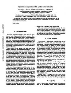
2 for a fault-tolerant implementation of the “high-level” location (i.e., logical state preparation, gate or measurement), followed by those locations needed for a full errorcorrection cycle. If the error rate for elementary operations is below the accuracy threshold, this replacement will result in an encoded circuit whose effective noise rate is lowered with respect to the original unencoded circuit. To lower the noise still further, the replacement procedure can be repeated sufficiently many times for the locations in the encoded circuit itself. Each time, a new circuit is created which is encoded at an increasingly higher level of a concatenated quantum code. Although this standard concatenation procedure is not necessarily the most efficient procedure for achieving fault tolerance, we will use it for the present study as its performance has been quantified both numerically and analytically in a number of different settings. The standard concatenation procedure described above can be varied and optimized in various physical settings. For example, Knill [5] has shown that, in a setting where memory and qubit transport are essentially noiseless, a very inefficient strategy for the generation of ancilla states based on post-selection gives a threshold around 3 × 10−2 for depolarizing noise. On the other hand, in the more realistic setting for contemplated solidstate implementations, where memory has a noise level in the same range as gate operations and qubit transport must be accomplished by noisy swap gate operations, a different strategy relying less on ancilla post-selection seems to be the best. Such an approach has been analyzed by Aliferis, Gottesman, and Preskill (AGP) [9]— they find noise thresholds in this setting to be somewhat lower than 10−4 for stochastic noise. Svore, DiVincenzo, and Terhal (SDT) [11] analyze a variant of this setting with qubits constrained to lie on a fixed two-dimensional square geometry. By modifying and adapting the verification circuits of AGP to this lattice geometry, the penalty on the threshold found by SDT in this setting is only about a factor of two compared with the completely unrestricted geometry of AGP. In all of this work, measurement times and gate operation times have been assumed to be of the same order. In fact, it would seem that the value of the accuracy threshold depends crucially on this assumption: Most importantly, measurement is used in ancilla verification during error correction and, the longer measurement takes, the longer the ancilla qubits need to wait in memory while verification is completed. The problem is illustrated by Fig. 1, which shows a fragment of a circuit that extracts information about errors in the data block according to the scheme introduced by Shor [10, 12]. Roughly speaking, if measurement takes 1,000 gate operation times, the memory noise level would need to be 1,000 times below the gate noise level for the fidelity of the waiting ancilla to remain high enough and the accuracy threshold for gate noise to stay unchanged when slow measurement is

taken in consideration. Steane [6] has documented such a decrease of the noise threshold with increasing measurement time, although the effect on the threshold is not as severe as our simple argument implies. There are some physical systems in which the noise for qubit storage (and movement) may indeed be very low, so that measurement-based verification can be used very effectively to obtain high accuracy thresholds [5]. But in other settings (e.g., in solid-state schemes) it is expected that noise levels for gate operations, memory, and moving will be comparable; it would seem that the threshold for FTQC would then be severely compromised by long measurement times.  

data block

 

|0i 

•

•

•

|+i

•

|0i

 • |0i 

• |0i  

FE

Z

FE •

FE •

FE •

FE

X X X X

+1

FIG. 1: Fragment of an error correction circuit in which a “cat state” ancilla [10] is prepared, verified, coupled to the data, and then measured. The first three controlled-NOT (cnot) gates prepare a four-qubit “Schr¨ odinger cat” [10] ancilla state. The next two cnots and the measurement of Z ≡ σz comprise the verification of this ancilla. In this protocol, this measurement outcome must be known before the verified ancilla is coupled to the data block: If the measurement outcome is −1, the cat state is to be discarded and ancilla preparation is to be attempted again.

However, in this paper we show the opposite: Even in these settings, and unlike the conclusion drawn in [6], the threshold is hardly affected by long measurement times. This is so because, as we discuss below (point 2.), one can replace the non-deterministic verification protocol in Fig. 1 with a deterministic protocol that corrects errors in the verified ancilla. And importantly, this replacement results in an accuracy threshold comparable to that obtained with non-deterministic verification. But the full story involves a combination of existing and new ideas, that we now explain: 1. Use of Pauli frames. We did not comment above on the use of the measurements of X ≡ σx in Fig. 1. These measurement bits are combined to yield the code syndrome which indicates errors in the data block and the necessary recovery operation to invert them. For all codes used in FTQC, these recovery operations are tensor products of single-qubit operations in the usual Pauli group. It has been known for some time (e.g., see [5, 9])

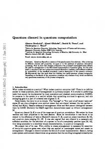
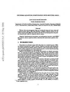
3 that it is not necessary to directly apply these recovery operations on the data. Instead, it is sufficient to merely record and keep track of them in a classical memory as a reference frame defined by a Pauli rotation. This is so because the Pauli group is closed under the action of the Clifford group: Pauli operators commute through gates belonging to the Clifford group to give other Pauli operators. Since gates in a fault-tolerant circuit that determine the accuracy threshold—most importantly, all gates needed for implementing error correction—belong to the Clifford group, the application of the recovery operations specified by the syndrome can usually be delayed a long time. 2. Ancilla decoding instead of verification. This is a new idea, and requires a modification of all existing ancilla verification circuits. But the modification is always simple—Fig. 2 shows the necessary change to the circuit in Fig. 1. The reason that ancilla pre-verification before interaction with the data has previously been considered necessary is that a single fault, at certain locations in the ancilla preparation circuit, can lead to a multi-qubit error in the ancilla state. It has therefore always been thought necessary to prevent such ancillae from interacting with the data. But, if the nature of these multi-qubit errors can always be determined by post-processing of the ancilla after its interaction with the data, then a suitable recovery operation can always be devised. The decoding and measurement of the ancilla in Fig. 2 serve to determine such a recovery operation for the data, and this operation is again always a tensor product of single-qubit Pauli operations. Therefore, as in our discussion above, correction of multi-qubit errors in the ancilla can always be delayed by incorporating the recovery operation into the Pauli frame. The Supplementary Information gives further details of this method.  

data block

 

|0i  •

|+i

•

|0i

 • |0i 



• •

• •

• •

•





FE

FE

FE

FE

Z X Z Z

FIG. 2: The modified circuit from Fig. 1: ancilla verification is removed, and is replaced by a decoding and measurement of the ancilla.

The remaining ideas are needed only to deal with these non-Clifford operations which, together with Cliffordgroup operations, complete quantum universality. NonClifford operations require a different treatment since a Pauli frame cannot be simply propagated through them:

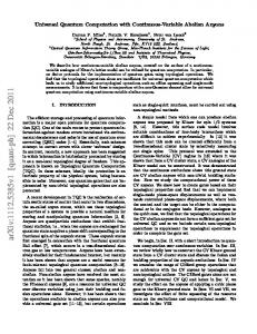
Commuting a Pauli operator through such a gate can generally give an operator outside the Pauli group. For this reason, all information determining the current Pauli frame must be known before the application of a nonClifford gate, so that the restoration operation can be applied immediately before the non-Clifford operation is implemented. We will now show that, despite this restriction, nonClifford gates can be executed effectively even when all measurements are slow. First, we recall that logical nonClifford gates are fault-tolerantly simulated using appropriate ancilla states. Non-Clifford gate operations appear in the sub-circuits preparing these ancillae, while the use of the ancillae after preparation and verification involves only Clifford-group operations [13]. This does not immediately lead to a solution to the measurement-time problem, as e.g. Fig. 3 illustrates. This figure shows how to simulate the T ≡ exp(−i π8 σz ) gate, with the Cliffordgroup gate S = T 2 conditioned on the measurement outcome. Alternatively, the logical Toffoli gate could be simulated, with cnot gates being conditioned on the measurement outcomes inside the simulation circuit [4, 10]. |ψi |aπ/8 i

•

S



FE

T |ψi

Z

FIG. 3: Simulation of the gate T using the ancilla |aπ/8 i ≡ T σx |0i, Clifford-group operations and measurement. The gate S is performed only if the measurement outcome is −1.

The simulation circuit of Fig. 3 is to be used in an encoded form and the ancilla block will be prepared in the logical |aπ/8 i state. And, as the next step, this circuit will also be concatenated in order to decrease the effective noise for the logical T gate to the desired level. When the simulation of the logical T gate occurs at level ℓ, the circuit in Fig. 3 uses a level-ℓ |aπ/8 i ancilla. And there is a fault-tolerant rectangle (see [9, 11] for the circuit) which prepares the level-ℓ ancilla using level-(ℓ−1) T gates. In this standard approach, these alternating replacements are iterated until Fig. 3 is used at level 1, where it contains zeroth-level physical T gates. However, this circuit is clearly unusable at level 1 if measurements are slow: The data qubits will have to wait in memory too long since the outcome of the measurement of level-1 logical Z (including all the preceding Pauli-frame information that determines its meaning) must be known in order to decide if the level-1 logical S gate is to performed (this decision must be made before this qubit is involved in the next logical cnot in the circuit, which is usually immediately). Is there a fix to this problem? Here is the essential idea: In order to get a very low effective error rate for the logical T gate, it is only necessary that the circuit of Fig. 3 appears at sufficiently many

4 high levels of concatenation. But at high levels of concatenation there is no problem with slow measurement! This is easy to see for concatenated error correction: the (k) gate time tgate at level k of concatenation scales expo(k)

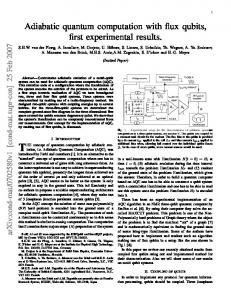
nentially with k, tgate = aC k for some constants a and C. On the other hand, the measurement time tmeas is the same at every level of concatenation, since logical measurement is performed by transversal measurements on the physical level. So, even if tmeas = 1000a and for, e.g., C = 34 (as in [11]), measurement is completed in one logical gate time for all k ≥ kmin = 2 & logC k. The more general idea is that at some level of coding, because the effective error rate for logical Clifford-group operations decreases quickly with coding level, the probability for a logical error in memory in the data block in Fig. 3 can be made sufficiently small for the total time it takes to measure the ancilla-block qubits. This can provide a more general criterion for determining kmin in cases where a strategy other than strict concatenation is used, or when C is quite small (C = 5 in [9]). To avoid dealing with the T gate at levels lower than kmin , we need an alternative to the iterative replacement described above. One has already been suggested in the literature (see e.g. [5]); it is referred to as 3. Injection by teleportation, and this is the last ingredient that we need. Fig. 4 illustrates the idea: The two logical |0i (|¯ 0i) blocks together with the logical Hadamard and cnot gates create a logical Bell pair for teleportation. This logical level corresponds to kmin . Then one of the code blocks of the Bell pair is decoded to the physical (unencoded) level. Next, a Bell measurement is done at the physical level between a qubit prepared in the |aπ/8 i state and the decoded half of the Bell pair. As a result, up to a Pauli-frame change P , the output block is in the logical |aπ/8 i (|aπ/8 i) state as desired. The noise level on the |aπ/8 i state, which has thus been injected into the level-kmin code block, will not be much greater than that of the original |aπ/8 i state and the physical noise level for Clifford operations (see e.g. [11]). |aπ/8 i |¯ 0i |¯ 0i

• / /

H

•



D



FE

FE

because there are two changes that slow measurements make for the threshold analysis neither of which should cause a major change in the threshold value: i) The circuits will be changed in detail in order to avoid ancilla verification. These changes are not major and, because the method of ancilla decoding is more efficient than verification, we expect the accuracy threshold to improve by a factor of around two by this change (see the Supplementary Information). In any case, this modification can be restricted only to levels less than kmin since, as discussed, slow measurement is not a problem at levels k ≥ kmin . ii) In the “local” setting of SDT, where qubits must be moved using swap gates on the two-dimensional lattice, extra space must be left for qubits to be measured (since they must remain in place for, say, 1000 time steps before they can be re-used). This requires an expansion of the physical patch of the lattice occupied by one logical qubit at the lowest level of concatenation. We estimate that this increases the linear scale of the computer by a small factor of around two, leading to perhaps a factor of two decrease of the threshold. The combined effect of (i) and (ii) leads us to expect that the accuracy threshold value will be only very minimally be affected in the slow-measurement setting. To conclude, we have shown that fault-tolerant quantum computation can be implemented in such a way that, except for minor effects, slow quantum measurements have no effect on the noise threshold at which error correction becomes effective. Our result does not apply to every existing scheme for FTQC; for example, it cannot be used in post-selected computation [5], and it does not apply to the (nondeterministic) quantum computation scheme that is possible in a linear-optics setting [14]. But in the situations generically envisioned in many implementations of quantum computing (the solid state ones, in particular), slow measurement will not be harmful. We thank Daniel Gottesman and Barbara Terhal for discussions. PA is supported by the NSF under grant no. PHY-0456720. DDV is supported by the DTO through ARO contract number W911NF-04-C-0098.

• X

• Z

P

|aπ/8 i

FIG. 4: Creation of the logical ancilla |aπ/8 i by teleportation.

The time required for implementing this circuit is independent of tmeas and, since injection occurs at level kmin , all measurement outcomes will be available in one logical gate time. With these observations, the threshold analyses of AGP and SDT go through essentially unchanged, so that the accuracy threshold is not effected in the slow-measurement setting. We say “essentially”

[1] D. Aharonov and M. Ben-Or. p. 176 in Proc. 29th Annual ACM Symposium on the Theory of Computation (1998, ACM Press, New York). [2] E. Knill, R. Laflamme, and W. Zurek. Proc. R. Soc. Lond. A, 454:365–384, 1997. [3] A. Kitaev. Russian Math. Surveys, 52:1191, 1997. [4] J. Preskill. pp. 213–269 in Introduction to Quantum Computation, eds. H.-K. Lo, S. Popescu and T.P. Spiller (1998, World Scientific, Singapore). [5] E. Knill. Nature, 434:39–44, 2005. [6] A. M. Steane. Phys. Rev. A, 68:042322, 2003. [7] L. Vandersypen, private communication. [8] A. Kitaev. Ann. Phys., 303:2–30, 2003. [9] P. Aliferis, D. Gottesman, and J. Preskill. Quant. Inf.

5 Comput. 6(2), 97–165, 2006. [10] P. W. Shor. p. 56 in 37th Annual Symposium on Foundations of Computer Science (FOCS ’96), 1996. [11] K. M. Svore, D. P. DiVincenzo, and B. M. Terhal. quantph/0604090. [12] D. P. DiVincenzo and P. W. Shor. Phys. Rev. Lett. 77, 3260–3263, 1996. [13] D. Gottesman, I. L. Chuang. Nature 402, 390–393, 1999. [14] E. Knill, R. Laflamme, and G. J. Milburn. Nature 409, 46–52, 2001.

6 Supplementary Information The need for ancilla verification—In the theory of quantum fault tolerance there are two well-known methods for performing fault-tolerant error correction. The first, due to Shor [10] and DiVincenzo and Shor [12], makes use of ancillae encoded in the classical repetition code informally called “cat” states. The second, which is due to Steane [A. Steane, Phys. Rev. Lett. 78, 2252 (1997).] and applies to the Calderbank-Shor-Steane (CSS) class of quantum codes, uses as ancillae logical |0i and |+i states encoded in the same code as the data. In both methods, the preparation of these ancillae by directly executing their encoding circuit is not in general a fault-tolerant procedure, and extra steps are needed before the ancillae are considered pure enough to be coupled to the data. This purification procedure, also known as verification, is performed by running parity checks on the ancilla using additional ancillary verifier states. Ancilla verification is typically done nondeterministically by simply rejecting ancillae that fail the parity checks of verification and starting anew. This procedure however is disadvantageous when measurement is slow since the verified ancilla qubits will have to be stored for long times in memory before measurements that are part of verification finish. Alternatively, verification can be done deterministically by correcting errors in the verified ancilla and thus avoiding post-selection. (Note that the deterministic protocol in Fig. 4 in [11] that does not correct errors in the ancillae is unusable when measurement is slow: In this protocol, an element of non-determinism exists in which ancillae are to be coupled to the data depending on the verification measurement outcomes.) The price for a deterministic verification procedure is a penalty in efficiency: A larger number of verifier qubits and verification operations are needed compared to the non-deterministic procedures (e.g., compare the deterministic protocol in Fig. 9 in [4] with the non-deterministic one in Fig. 11 in [9]). And this increase in qubit and operation overhead translates into a decrease in the accuracy threshold as compared to non-deterministic verification—this is the reason why non-deterministic verification has been used hitherto in almost all threshold studies. We will here describe how ancilla verification can be avoided altogether and replaced by suitable decoding of the encoded ancillae after these interact with the data during error correction. We find that not only does this method improve the efficiency of present schemes that use verification, but it also leads—in the examples of interest we have studied in detail—to an improvement in the accuracy threshold as compared even to non-deterministic verification procedures. We will first discuss the case of distance-3 quantum codes correcting arbitrary errors on any one qubit in the code block. In the end we will discuss the generaliza-

tion to codes of higher distance. Throughout, we use the shorthand notation X ≡ σx and Z ≡ σz and we also use superscripts to denote the qubit on which an operator acts (e.g., Z (i) denotes a Pauli σz operator acting on the i-th qubit). Ancilla decoding instead of verification—The intuition leading to this method is guided by a few basic observations on how fault-tolerant error correction is implemented. The first observation is that ancilla verification checks particular error patterns and does not need to protect against arbitrary multi-qubit errors. In particular, we are concerned with faults that appear in first order in the encoding circuit and propagate to cause multi-qubit errors at the output of the ancilla encoder that our distance-3 code cannot correct. Verification works by exactly trying to detect (or correct, in deterministic schemes) these particular errors appearing in first order, with the additional condition that the verification step should not, also in first order, introduce multi-qubit errors in the ancilla that is being verified. The second observation is that the ancilla after interacting with the data block remains, ideally, in a known logical state. For example, √ after the cat state ¯ rep ≡ (|00 . . . 0i + |11 . . . 1i)/ 2 interacts with the |+i ¯ rep or |−i ¯ rep (the data, it remains encoded in either |+i latter differs by the sign having flipped from + to − in the above superposition). Similarly in Steane’s error correction method, an ancilla prepared in the logical |0i state remains in the same state after interacting with the data. This is more information than just knowing that the ancilla state is protected by a code—we have additional information about what the state should be. The idea of the new method is to couple the encoded ancilla to the data without attempting any verification, followed by a procedure that is run afterwards on it and allows us to learn and invert possible multi-qubit errors produced by the encoder and having propagated to the data. This procedure could be implemented in various ways, but it seems that the most efficient (and eyepleasing) one is via a suitable decoder. A schematic of this method is given in Fig. 5. To prove that this error-correction (EC) method is fault tolerant, we need to show that properties 0′ , 0 − 2 in [9] are satisfied. Properties 0 (EC without faults takes an arbitrary input to the code space) and 1 (EC without faults corrects single-qubit errors in the data block) are true since, without faults, verification is superfluous and the measurement outcomes after decoding will give the necessary syndrome information to perform ideal error correction. Properties 0′ (EC with one fault always produces an output deviating by at most a weight-one operator from the code space) and 2 (EC with one fault produces a block with at most one error if the input has no errors) require proof. As with the known errorcorrection methods that use ancilla verification, showing

7 data block



/ |0i⊗k

/ D

|ψenc i

−1

•

/ D

FE

{xi }

FE

¯ L

FIG. 5:

Schematic of fault-tolerant error correction without ancilla verification for distance-3 codes. The ancilla is encoded by starting with ancillary qubits in a reference state (e.g., |0i⊗k ), the state to be encoded (|ψenc i), and running the unitary encoding circuit (D −1 ). After interacting with the data block (schematically shown as a cnot), the ancilla is decoded using a unitary decoding circuit (D). The final measurements yield syndrome information ¯ ({xi }) and the eigenvalue of a logical operator (L).

that property 0′ holds is made easier after understanding why property 2 is satisfied. And as we will see, satisfying property 2 will determine how our decoding circuit must be designed. What we need to show is that a single fault in the EC circuitry cannot cause more than one error in the corrected data block (which for property 2 initially has no errors). Consider first the case where the fault occurs during the interaction with the data. Since this interaction is done with transversal gates, no gate operates on more than one qubit in the same block. Therefore a single fault cannot cause more than one error in the data. An error can also appear in the ancilla block, but this does not prevent successful correction: If cat states are used the syndrome extraction is repeated, or in Steane’s method the errors in data and ancilla blocks occur always in the same qubit in the code block and a single syndrome extraction can be trusted. The second case is when the fault occurs inside the ancilla encoder. In general the encoding circuit has no special structure and more than one errors can appear in the produced encoded ancilla. The encoder can however be designed so that no logical error appears at the output due to a single fault inside it and, furthermore, the possible error patterns caused by all such first order fault events are known. Of interest are multi-qubit errors which may propagate to the data via the ancilla-data interaction. However, letting ancilla and data interact without verification as in Fig. 5 is permissible since the information at the output of the following decoder will allow us to diagnose whether such error propagation did occur and invert it. To understand how this is possible, it is useful to think of the decoding circuit as performing error correction while simultaneously decoding its input block to a qubit. Since in the case considered the decoder is fault-free, both processes are executed ideally. The decoder then performs the mapping Ei |¯0i → |ii ⊗ |0i ; Ei |¯ 1i → |ii ⊗ |1i ,

(1)

where {Ei } is the set of all single-qubit Pauli errors that our distance-3 code corrects, |¯ 0i (|¯ 1i) is the ideal logical

|0i (|1i) state, and i is syndrome information that, after decoding, indicates the error Ei (if the code is not perfect and the basis {Ei |¯0i, Ei |¯1i} does not span the whole Hilbert space, the action of the unitary decoder can be extended to include some non-correctable errors). Now, if we decode a n-qubit cat state, then measuring the qubits carrying the syndrome will allow us to learn all eigenvalues of the Z (i) Z (j) code stabilizers for 1 ≤ i = j − 1 ≤ n − 1. Hence we can diagnose whether multi-qubit X errors were produced in the encoder and can invert them by updating the Pauli frame of the data block. In Steane’s method, the syndrome information will diagnose any X (resp. Z) errors in the logical |0i (resp. |+i) ancilla that propagate to the data. In addition, measuring the decoded qubit (the second tensor¯ in Fig. 5) will product factor in Eq. (1); denoted by L reveal the eigenvalue of the logical Z (resp. X) operator. This resolves the ambiguity about the error causing a particular syndrome since, for Ei and Ej to have the same ¯ where O ¯ is either trivial (equal to syndrome, Ei† Ej = O ¯ or anti-commutes with L. ¯ Thus, either the identity or L) Ei and Ej are equivalent up to an element of the ancilla stabilizer, or lead to orthogonal decoded states which allows distinguishing them. Again, whenever multi-qubit errors are detected, the appropriate Pauli-frame change is done on the data block to invert them. The final case to consider is when a single fault occurs in the decoding circuit. In the case discussed above we were concerned with correcting multi-qubit errors caused by a single fault in the encoder and subsequently propagating to the data. But we also need to guarantee that such a corrective step is not mistakenly taken due to a single fault inside the decoder (which can cause no errors to the data block). Thus, to satisfy property 2, we must ensure that no single fault inside the decoding circuit can give the same syndrome (including the eigenvalue of the ¯ as any of the multi-qubit errors which logical operator L) a single fault inside the encoder can produce. Constructing the decoding circuit to meet this condition must be done with care given the chosen ancilla encoder. In the examples section that follows such decoder designs are shown for some very frequently used cases: fault-tolerant measurements using four- and seven-qubit cat states and Steane’s error-correction method for the [[7,1,3]] code. We conjecture that an appropriate decoding circuit can be found for any distance-3 code. In any case, a less efficient but general solution is always possible: We can further encode the ancilla after interacting with the data in the two-bit classical repetition code and then decode the two sub-blocks separately as shown in Fig. 6. In this circuit, when the syndrome for X errors at the two sub-blocks agree, then we can be confident that, to first order, any detected multi-qubit X error has occurred during ancilla encoding and has propagated to the data. Otherwise, if the syndromes for X errors disagree, we conclude that, again to first order, a fault has

8 happened in one of the two decoded sub-blocks and no multi-qubit X error has propagated to the data. The syndrome for Z errors (revealing Z errors initially in the input data block) can be obtained by taking the parity of the syndromes at the two sub-blocks. data block



/ |0i⊗k

/ D

•

/

•

−1

D

|ψenc i |0i⊗(k+1)

 D

FE

{xi }

FE

¯ L

FE

{x′i }

FE

L¯′

FIG. 6:

To ensure that a single fault during ancilla decoding cannot be mistaken for a fault inside the ancilla encoder leading to the same syndrome, the ancilla is encoded in the two-bit classical repetition code and then the two sub-blocks are decoded separately. If the syndrome in both sub-blocks indicates a multi-qubit X error then we are confident a fault in the ancilla encoder occurred and propagated to the data. Otherwise the fault must have occurred during the decoding procedure.

For such designs that satisfy property 2, let us now discuss property 0′ . We observe that errors that may propagate from the encoder to the data block (e.g., X errors when ancilla and data interact via a cnot as in Fig. 5) are decoupled from errors that propagate the other way around (Z errors). Hence detecting and inverting errors caused in the encoder does not interfere with the way errors initially in the data are treated by EC. Therefore, the success of our method for dealing with single faults inside the EC circuitry is independent of whether the data block starts in the code space or not. This implies that EC methods which satisfy property 0′ when ancilla verification is used (e.g., Steane’s method as discussed in [9]), will still satisfy it if decoding of the ancilla is performed instead as described above. For non-perfect codes we need to worry also about replacing verification against multi-qubit errors that do not propagate from the ancilla to the data (e.g., Z errors in Fig. 5). (Recall that a code is called perfect if all possible syndromes point to correctable errors, as is e.g. the case for the Steane [[7,1,3]] and Golay [[23,1,7]] codes.) Verification against such errors can be easily avoided by repeating the syndrome extraction: The circuit in Fig. 5 or 6 can be repeated three times and the syndrome for Z errors in the data must only be trusted if at least two of the syndromes for Z errors agree. (The same applies for the X error correction.) Finally, one technical point must be addressed. With a single syndrome extraction as in Fig. 5, property 2 is satisfied separately for X and Z errors. That is, a single fault inside the ancilla encoder may lead to a single

X and a single Z error in the output data block with the two errors acting on different qubits inside the block. This is not a problem as long as the subsequent logical operation does not mix X and Z errors, as e.g. is the case for the logical cnot which are transversal for CSS codes. If however a logical S gate is applied next then we must enforce property 2 in a stricter sense and prevent X and Z errors acting on different qubits at the output of EC. This can be achieved by extracting the syndrome a second time by running the EC circuit again. This modification will have no effect on the accuracy threshold since the logical S gate can be handled via injection by teleportation [11]. A similar ancilla decoding technique can replace verification when EC uses a quantum code that corrects t > 1 errors. Now, properties 0 – 3 in §10 in [9] are sufficient to guarantee fault tolerance and our decoding circuit must be designed appropriately. Most importantly, we must ensure that, with k ≤ t faults inside EC, errors acting on more than k qubits that may propagate from the ancilla to the data can be diagnosed by the subsequent ancilla decoding and inverted. This can be accomplished by encoding the ancilla into a t-bit classical repetition code before decoding each sub-block separately similar to Fig. 6. For example, for the [[23,1,7]] Golay code that corrects t = 3 errors, ancilla decoding can replace verification if we encode the ancilla after interaction with the data into the 3-bit classical repetition code [B. Reichardt, Private communication.]. Some examples—We will now give some examples of this method in use. Let us begin with fault-tolerant syndrome measurement using four-qubit cat states, which is e.g. useful for EC with the [[5,1,3]] or [[7,1,3]] codes. The circuit for encoding, verifying and interacting these cat states with the data was shown in Fig. 1. An alternative circuit that performs the same measurement without ancilla verification was shown in Fig. 2. The circuit in Fig. 2 is fault tolerant because the error X (1) X (2) (or its equivalent X (3) X (4) ) which may appear in the encoder in first order will be detected as it leads to all three measurements of Z after decoding giving outcome −1. In addition, no single fault inside the decoding circuit can flip all three Z-measurement outcomes, something which would lead us to mistakenly cause a weight-two error in the data by applying an unnecessary correction. The second example is fault-tolerant measurement using seven-qubit cat states, which is e.g. needed for logical measurements that prepare ancilla needed for universality in the [[7,1,3]] code (see Figs. 13 and 14 in [9]). The circuit for encoding and verifying these cat states (Fig. 14 in [9]) is shown in Fig. 7. The verification can again be omitted if, after interaction with the data, the cat state is decoded with the circuit shown in Fig. 8. To understand how the outcomes of the final measurements of Z allow us to diagnose any

9 |0i



|0i



•

|0i



•

|+i

•

•

|0i



•

|0i



•

|0i



data block

•

−1 D|0i

−1 D|+i

•

FE

Z

+1

FIG. 7:

Encoding and verification of a 7-qubit cat state. Similar to Fig. 1, a verifier qubit is used to measure the parity Z (1) Z (7) on the ancilla. Any of the high-weight X errors (X (1) X (2) , X (6) X (7) , X (1) X (2) X (3) , or X (5) X (6) X (7) ) created in the encoder in first order is thus detected before the ancilla interacts with the data.

multi-qubit X errors having resulted from a single fault in the ancilla encoder, we follow the propagation of these errors through the decoding circuit: → → → →

X (1) X (2) X (6) X (6) X (7) X (1) X (2) X (3) X (6) X (7) X (2) X (4) X (6) X (7)

(2)

An X error appearing on the right-hand side of Eq. (2) will result in the measurement of Z on the corresponding qubit giving an outcome −1. We note that different initial errors propagate to different final error patterns and, hence, distinct measurement outcomes which allows distinguishing them. In addition, it is straightforward to see that no single fault inside the decoder can lead to any of the final error patterns in Eq. (2). So no fault inside the decoder can make us mistakenly apply a multi-qubit correction to the data.  •

 

• •

• •

 

D|0i

•



D|+i

FIG. 9:

|0i  

X (1) X (2) X (6) X (7) (1) (2) (3) X X X X (5) X (6) X (7)

 •

FE

FE

FE 

FE •

FE

FE

FE

Z Z Z Z X Z Z

FIG. 8:

The decoding circuit that replaces verification for the 7-qubit cat state prepared as in Fig. 7. The outcome of the measurement of X on the fifth qubit gives the eigenvalue of the measured operator on the data. As in Fig. 2, all measurements of Z give ideally outcome +1.

Our third example is fault-tolerant EC using Steane’s method for the [[7,1,3]] code. In this method, logical |0i

Steane’s EC without ancilla verification for the [[7,1,3]]. −1 The encoding circuit for the |0i state (D|0i ) is shown separately in Fig. 10, and the corresponding decoder, which here includes the final measurements, (D|0i ) in Fig. 11. The encoder and decoder for the |+i state are identical with the direction of the cnot gates reversed and with qubit preparations and measurements performed in the conjugate bases.

and |+i states are sequentially coupled to the data block to extract the syndrome information. In Steane’s original scheme each ancilla is verified by either comparing two independently-encoded ancilla copies or by measuring suitable parities with extra verifier qubits (for the [[7,1,3]] code the measurement of a single parity is sufficient; see [11]). In our variant of this method no verification is performed and after encoding the ancilla is allowed to interact with the data. The decoding circuit that is applied next to the ancilla is identical with the encoding circuit. A schematic of this EC method is shown −1 in Fig. 9, where the encoder (D|0i ) and decoder (D|0i ) of the logical |0i state are shown separately in Fig. 10 and Fig. 11, respectively. To show the tolerance of this design to single faults, we first list the possible multi-qubit X errors produced −1 in first order in the encoder D|0i : X (1) X (7) , X (2) X (3) , and X (4) X (5) . Propagating them through the decoding circuit of Fig. 11 we obtain X (1) X (7) → (X (1) )X (3) X (5) X (2) X (3) → (X (2) )X (6) X (7) , X (4) X (5) → (X (4) )X (6) X (7)

(3)

where we have put in parenthesis trivial errors acting on qubits subsequently measured in the X eigenbasis. As seen in Eq. (3), the first weight-two error gives a distinct syndrome from the other two, which have identical syndromes (they both flip the eigenvalues of the measurements of Z on the sixth and seventh qubit). This is however to be expected, because their product X (2) X (3) X (4) X (5) is in the code stabilizer and so the same recovery operator can be applied for both. Finally, it can be easily checked that the decoder is designed so that a single fault inside it cannot lead to any of the final error patterns in Eq. (3). Note that running the encoding circuit backwards would not have provided a decoding circuit with this property: Indeed, we can see that if e.g. the cnot gate from the second to the third qubit is applied in the first time step of the decoder, then it will not be possible to distinguish whether the error

10 |+i

•

• •

|+i |0i



|+i

•

•

•

 •

•



|0i |0i





 

|0i

X (2) X (3) was produced by a fault in the encoder or by this decoder cnot gate failing.

•





FIG. 10: Our encoder for the logical |0i state in the [[7,1,3]] code. Single fault events in this circuit can lead to weight-two X errors (X (1) X (7) , X (2) X (3) , or X (4) X (5) ), which will propagate to the data block through the transversal cnot gates of Fig. 9.

•

•

•

•

•





•

•

•







 

FIG. 11:

•





FE

FE

FE

FE

FE

FE

FE

X X Z X Z Z Z

Our decoder for the logical |0i state in the [[7,1,3]] code corresponding to the encoder of Fig. 10. The measurements of X yield the syndrome for Z errors in the data block, while all measurements of Z give ideally outcome +1.

Conclusion—Avoiding ancilla verification is helpful when measurements are slow since measurement outcomes need not be available immediately. Furthermore, the EC circuits become more efficient in both the number of qubits and operations compared to the EC circuits that use ancilla verification. For example, using this new method to perform EC inside the [[7,1,3]] cnot-exRec in [9] decreases the total number of locations from 575 to 351 and the number of ancillary qubits by half. Counting malignant pairs in the new circuit nearly doubles the accuracy threshold lower bound found in [9] which changes from 2.73 × 10−5 to 5.36 × 10−5 . This method may also prove beneficial for fault tolerance with geometric locality constraints since the reduction in the number of qubits will result in a smaller unit cell and so shorter movement. Finally, we would like to comment that it would be interesting to investigate whether a similar ancilla decoding technique can replace verification in the teleported errorcorrection method discussed in [5].