Journal of Marine Science and Technology, Vol. 23, No. 3, pp. 353-363 (2015 ) DOI: 10.6119/JMST-014-0327-7
353
EFFECTS OF VARIOUS EXTRAPOLATION TECHNIQUES FOR ABBREVIATED DYNAMIC MODULUS TEST DATA ON THE MEPDG RUTTING PREDICTIONS Minkyum Kim1, Louay N. Mohammad2, and Mostafa A. Elseifi3 Key words: abbreviated dynamic modulus test, time-temperature superposition, shift factor, Arrhenius, Williams-LandelFerry (WLF), Kaelble, quadratic function, extrapolation, MEPDG.
ABSTRACT Abbreviated dynamic modulus test protocols have been used to reduce the time and cost of running the test for routine uses. The abbreviated test results can then be extrapolated to estimate the complete array of the dynamic modulus values required for the Level 1 MEPDG analysis. Multiple approaches are available for the extrapolation depending on a master curve and shift factor functions chosen. The objective of this study was to identify the best practice of extrapolating the abbreviated dynamic modulus data by evaluating the accuracy of performance predictions through MEPDG pavement analysis. Two common sigmoid functional forms (i.e., the MEPDG Sigmoid and a Generalized Logistic functions) were compared for master curve construction. Four different shift factor functions were used to estimate the shift factors beyond the abbreviated temperature limits. The Arrhenius, WilliamsLandel-Ferry (WLF), modified WLF by Kaelble, and quadratic functions were investigated. Through extrapolation, significant underestimations of the dynamic modulus values at 54.4°C were obtained from all eight approaches. Among the eight approaches, the Generalized Logistic function coupled with the quadratic shift factor function showed relatively lower extrapolation errors. On the other hand, the MEPDG performance predictions using the eight sets of extrapolated dynamic modulus input showed less than 1 mm differences in
Paper submitted 12/23/13; revised 01/13/14; accepted 03/27/14. Author for correspondence: Louay N. Mohammad (e-mail:
[email protected]). 1 Louisiana Transportation Research Center, USA. 2 Louisiana Transportation Research Center and Department of Civil and Environmental Engineering Louisiana State University, USA. 3 Department of Civil and Environmental Engineering Louisiana State University, USA.
the terminal rut depth when compared to the performance predictions using the measured data sets.
I. INTRODUCTION Dynamic modulus, an absolute value of complex modulus under axial loading (|E*|), is a fundamental mechanical property describing the viscoelastic characteristics of asphalt mixtures. It was adopted as a key material input in the Mechanistic-Empirical Pavement Design Guide (MEPDG) developed under National Cooperative Highway Research Program (NCHRP) 1-37 (NCHRP, 2004). A standard test procedure, AASHTO T342 “Standard Method of Test for Determining Dynamic Modulus of Hot-Mix Asphalt Concrete Mixtures,” requires a full sweep of testing at five temperatures and at six loading frequencies on a 100-mm-diameter and 150-mm-tall specimen under uniaxial compression for a complete viscoelastic characterization of a mixture. With the full spectrum of dynamic modulus data of asphalt mixtures provided, the MEPDG analysis software, currently marketed as “PavementME,” numerically computes the stress-strain state in a pavement structure during the design life and predicts the level of distresses in the pavement from the computed stress-strain responses through empirical transfer functions across a wide range of pavement temperatures and loading frequencies. Therefore, the MEPDG analysis software requires that the complete set of dynamic modulus data is defined for accurate pavement performance predictions. In fact, for the highest hierarchical order of the analysis (Level 1), current version of the MEPDG software only accepts a complete array of dynamic modulus data (i.e., five temperatures by six frequencies, [56], as specified in AASHTO T342) as the asphalt layers’ material input. Often times, however, it is desirable or necessary that the dynamic modulus test of asphalt mixtures be conducted at a reduced number of temperatures and/or frequencies (Kim et al., 2004; Bonaquist, 2008; McCarthy and Bennert, 2012). From a practicality standpoint, it is desirable to reduce the time required to complete one set of dynamic modulus tests for
Journal of Marine Science and Technology, Vol. 23, No. 3 (2015 )
routine uses by highway agencies. Further, for evaluation of field compacted mixtures with thickness around 50-mm or less, it is necessary to perform the test under indirect tension (IDT) mode, which may experience higher test variability at high test temperatures due to the biaxial nature of the stress state in the specimens. To address these issues, abbreviations in the number of test temperatures and modifications to loading frequencies of AASHTO T342 have been proposed by many researchers in recent years (Kim et al., 2004; Bonaquist, 2008; You et al., 2009; Kim and Buttlar, 2010; McCarthy and Bennert, 2012). In order to run a pavement analysis or performance prediction through the Level 1 MEPDG simulation, the standard [56] array of dynamic modulus input should be obtained from the array of abbreviated test results using an extrapolation technique, which necessitates the use of a source function to construct a dynamic modulus master curve and another function to define a shift factor-temperature relationship. Multiple functional forms are available in the literature (NCHRP, 2004; Rowe et al., 2009; Yusoff et al., 2011) for both the master curve and the shift factor-temperature relationship, and depending on the selection of the functions, the extrapolation process results in different dynamic moduli outside the measurement range. When the high temperature dynamic modulus values are to be extrapolated, the difference in the extrapolation may have considerable effects on the rutting performance prediction at high service temperature by the MEPDG software. Thus, it is important to understand how accurate the extrapolation of the dynamic modulus can be with different combinations of master curve and shift factor functions.
II. OBJECTIVE AND SCOPE The objective of this study is to identify the best practice of extrapolating the abbreviated dynamic modulus data by evaluating the accuracy of performance predictions through MEPDG pavement analysis. Two popular sigmoid functional forms were used to construct master curves of asphalt mixtures. The first form is the well-known sigmoid function used in the MEPDG (NCHRP, 2004) and the second form is a generalized logistic function originally developed by Richards (1959) for plant growth modeling, then later used by Rowe et al. (2009) for master curve construction. Four different shift factor functions were used to estimate the horizontal shift factors beyond the temperature limits of the abbreviated test data. The Arrhenius, Williams-Landel-Ferry (WLF), a modified WLF function by Kaelble (1985), and a quadratic function were the four functional forms investigated in the study.
III. BACKGROUND 1. Dynamic Modulus Test Protocols For a comprehensive characterization of time and temperature-dependent behavior of asphalt mixtures, dynamic moduli need to be measured at multiple temperatures and at
Dynamic Modulus |E*|, ksi
354
1E+4
γ
α +δ
1E+3
β
1E+2
δ
Measured Master Curve
1E+1 1E-7 1E-5 1E-3 1E-1 1E+1 1E+3 1E+5 1E+7 Loading Frequency (Hz)
Fig. 1. Time-temperature superposition and master curve construction example.
multiple loading frequencies as shown in Table 1. The standard test protocol, AASHTO T324, specifies five temperatures and six loading frequencies. For better implementation in routine test practices, Bonaquist (2008) developed an abbreviated test protocol to shorten the time required to complete a suite of testing by eliminating tests at two extreme temperatures and a few loading frequencies. Thus, the standard [56] test matrix is reduced to a more concise [33(4)] test matrix. One additional frequency test at 0.01 Hz is conducted at the highest temperature (35, 40, or 45C) to ensure sufficient coverage of the master curve across a wide range of reduced frequency. Bonaquist’s approach then utilizes an extrapolation procedure of the measured dynamic modulus data to obtain the standard [56] test matrix in order to generate the required MEPDG input data for the asphalt layers. In the proposed procedure, the MEPDG sigmoid master curve function and the Arrhenius shift factor function are used for the extrapolation along with the maximum dynamic modulus value estimated from the Hirsch model. Kim et al. (2004) compared dynamic modulus test results under indirect tension (IDT) mode at three temperatures and at eight loading frequencies, [38], to that of the standard test protocol developed under NCHRP 1-37A (NCHRP, 2004). The highest temperature was reduced to 35C, but two loading frequencies (e.g., 0.05 and 0.01 Hz) were added to make sure proper overlap between wider adjacent temperature tests. With the addition of the two frequencies, the entire coverage of the measured dynamic modulus data was very comparable to that of the standard test method, and an extensive extrapolation of the data was not required. Other combinations of temperatures and loading frequencies were also investigated depending on the purposes, regional conditions, practical limitations, and so on (You et al., 2009; Kim and Buttlar, 2010). 2. Master Curve Functions Measured dynamic modulus data at multiple temperatures and frequencies are used to construct a single master curve at a reference temperature to predict the time-dependent behavior of asphalt mixtures from nearly instantaneous to stationary loading conditions as shown in Fig. 1. As the loading frequency
M. Kim et al.: Effects of |E* | Extrapolation on MEPDG Rutting Predictions
355
increases on the horizontal axis of Fig. 1, the duration of the loading on a material becomes more instantaneous and vice versa. As shown in Fig. 1, the material becomes stiffer under instantaneous loading and gets softer as the loading gets slower. A master curve is constructed on a basis of the time-temperature superposition principle (TTSP) for linear viscoelastic materials that exhibit a thermorheologically-simple material behavior (Ferry, 1980; Christensen, 2003). Specifically, if a material is thermorheologically simple, then a change in temperature should equally affect the dynamic moduli measured at different loading frequencies, but at the same temperature condition. It results in a paralleled shift of a set of six data points measured at the same temperature as illustrated in Fig. 1. After shifting the five individual data sets, all the dynamic modulus data points form a single curve known as a master curve over a wide range of reduced frequencies. On a semi-log or a log-log scale, this modulus-frequency relationship of a typical asphalt material resembles a sigmoid curve. Therefore, any mathematical functions that are sigmoid can be used to model the dynamic modulus master curve of asphaltic materials.
Eqs. (1) and (2). The effect of the coefficient on the shape of the master curve was explained by Yusoff et al. (2011). When the equals to 1, Eq. (3) reduces to Eq. (1); the MEPDG sigmoid function.
1) MEPDG Sigmoid Function One of the most popular sigmoid functions for master curve construction of asphalt mixture is the one used in the MEPDG (NCHRP, 2004) as shown in Eq. (1):
1) Arrhenius The Arrhenius equation is one of the oldest functions used to explain the temperature-dependent processes or material properties. A general form of the Arrhenius shift factor function may be expressed as a linear combination of a constant and a product of a coefficient and a difference between reciprocals of a temperature and a reference temperature (Rowe et al., 2011). Numerous modified forms are available, but the most widely used functional form for asphaltic materials may be expressed as follows:
log( E * )
1 e
(1)
(log f r )
where |E*| is the dynamic modulus, is the minimum value of |E*|, is a range of the dynamic modulus as computed as the difference between a maximum value of |E*| and , and are shape parameters, and fr is the reduced loading frequency defined as follows: f r f a(T )
(2)
where f is the actual loading frequency at tests and a(T) is the horizontal shift factor for a set of dynamic modulus at temperature, T. 2) Generalized Logistic Function Rowe et al. (2009) evaluated a generalized logistic function originally developed by Richards (1959) for plant growth modeling in order to overcome the limited versatility of the MEPDG sigmoid function due to the symmetrical property of the function. The generalized logistic function is shown as:
log( E * ) (1
1
(3)
e (log f r ) )
where is a shape parameter to allow the curve to take a non-symmetrical shape and other parameters are as defined in
3. Shift Factor Functions As previously mentioned, thermorheologically simple materials should have a constant shift factor for the moduli measured at the same temperature, and thus, the shift factor can be expressed as a function of temperature. The relationship is generally regarded as non-linear(Yusoff et al., 2011; Rowe et al., 2011). Some popular shift factor functions that can be used to describe the shift factor-temperature relationship include the Arrhenius, Williams-Landel-Ferry (WLF), Kaelble’s modified WLF, and a quadratic function. None of these functions describe the shift factor-temperature relationship fundamentally, nor predict the shift factors without the knowledge of the materials tested. Since these relationships are empirical, the fitting parameters must be pre-determined experimentally for all four function forms.
log a(T )
0.4347 Ea R
1 1 T Tref
(4)
where Ea is an activation energy used as a regression constant, R is the universal gas constant, T is the temperature in Kelvin (K), and Tref is the reference temperature. 2) Williams-Landel-Ferry (WLF) The WLF equation is a widely recognized shift factor function used for asphaltic materials as shown in Eq. (5): log a(T )
C1 (T Tref ) C2 (T Tref )
(5)
where C1 and C2 are constants, which are believed to have specific values for most asphaltic materials. However, recent results [8] reported that numerically obtained values of the constants for a wide range of asphalt materials are not consistent, but varies within considerably wide ranges. 3) Modified WLF by Kaelble A modification to the WLF function was proposed by
356
Journal of Marine Science and Technology, Vol. 23, No. 3 (2015 )
Kaelble (1985); Rowe et al. (2009) recently attempted to use the modified WLF function for asphaltic materials to provide more flexibility in fitting the highly non-linear shift factors at extreme temperature conditions. The modification was proposed by introducing an inflection point in the curve as follows: T T Tref Td d log a (T ) C1 C2 T Td C2 Tref Td
(6)
where Td is a defining temperature for the inflection point, and other parameters are as defined earlier. For asphalt mixtures, Td was found to range from 10C to 35C. 4) Quadratic Function A generalized second-order polynomial (quadratic) function was proposed in the literature (Rowe et al., 2011) for modeling the shift factor-temperature relationship as follows: log a (T ) T 2 T
(7)
where , , and are fitting parameters. The quadratic equation is a simple function, yet it fits very well to the observed shift factor data over a considerably wide range of temperatures. One weakness of this function is that it does not have a strong theoretical basis. However, the quadratic function is worth considering given that the other three shift factor functions are not free from empiricism as presented in Eqs. (4) to (6). Another issue to take into account is that Eq. (7) will violate the boundary condition (i.e., log a(T) = 0 when T = Tref) when it is used to predict the shift factors for non-observed temperatures with the fitting parameters determined in the measurement range. Eq. (7) was modified by replacing the independent variable with the difference between the test temperature (T) and the reference temperature (Tref) and by eliminating the constant term at the end as shown below: log a(T ) (T Tref ) 2 (T Tref )
(8)
Eq. (8) has two fitting parameters, , and , that need to be determined from the observed data.
IV. EXTRAPOLATION APPROACHES As shown in Table 1, abbreviated dynamic modulus tests can be performed at different combinations of test temperatures and frequencies under either uniaxial or IDT mode. In this study, the standard dynamic modulus test protocol (i.e., [56] matrix) has been used under uniaxial compression as the primary asphalt mixture performance test (AMPT). In addition, the abbreviated dynamic modulus tests have been conducted under IDT mode at three temperatures (e.g., -10, 10,
Table 1. Dynamic modulus test protocols. Loading Frequency (Hz) AASHTO T324 -10, 4.4, 21.1, 37.8, 54.4 25, 10, 5, 1, 0.5, 0.1 Bonaquist (2008) 4, 20, 35 ~ 451) 10, 1, 0.1, (0.01)2) 25, 10, 5, 1, 0.5, 0.1, Kim et al. (2004) -10, 10, 35 0.05, 0.01 1) Highest temperature varies depending on the asphalt binder high temperature PG. 2) 0.01 Hz test is conducted only at the highest temperature. Test Method
Temperature (°C)
Abbreviated dynamic modulus Determine Tref
Constructing Master curve
Store master curve fitting parameters
Obtained shift factors
Fitting shift factors to a given function
Store shift function fitting parameters
Calculating a full array of dynamic modulus |E*|= F(T, f ) Fig. 2. Details of the extrapolation procedure.
and 30 or 35C) and six loading frequencies (10, 5, 1, 0.5, 0.1, and 0.01 Hz), [36], which needed to be extrapolated. Fig. 2 illustrates a general procedure to obtain a full sweep of dynamic modulus data from an abbreviated set of test results by extrapolations. Starting with the measured dynamic modulus data of the [36] matrix, a master curve is constructed at a pre-determined reference temperature (Tref). Master curve fitting parameters along with the shift factors at each of the three temperatures are obtained. The obtained shift factors are then fitted into a shift factor function and the function parameters are determined. Using the master curve equation coupled with the shift factor equation as a function of the temperature (T) and frequency ( f ), the dynamic moduli for the complete temperature and frequency combinations are estimated. The extrapolation process is basically a series of numerical optimization through the least-square curve fitting technique. The Excel Solver function is one of the most widely used tool for the numerical optimization and was adopted in this study.
M. Kim et al.: Effects of |E* | Extrapolation on MEPDG Rutting Predictions
Table 2. Asphalt mixtures and field projects.
LA964 Baker
I10 Egan
I10 Vinton
Built Year
2005
2004
2003
Mix ID LA964 BK WC LA964 BK BC I10 EG WC I10 EG BC I10 VT WC
Thickness (mm)
Lift Wearing
40.0
Binder
110.0
Wearing
50.8
Binder
189.0
Wearing
50.8
Asphalt binder Grade PG76 -22M PG76 -22M PG76 -22M PG76 -22M PG76 -22M
1E+5 NMAS (mm) 19 25 12.5 25 12.5
Table 3. Extrapolation techniques as master curve-shift factor combinations.
Dynamic Modulus (MPa)
Project Location
357
I10 EG WC 1E+4 Tref = 25°C 1E+3 General Logistic 1E+2 1E-12
MEPDG Sigmoid 1E-8
1E-4
1E+0 1E+4 fred (Hz)
1E+8
1E+12
Fig. 3. Effects of source functions on master curves: I10 EG WC mixture.
extrapolation methods on the rutting performance predictions of two pavement sections (i.e., LA964 Baker an I10 Egan).
Shift Factor Functions MEPDG Master Curve Sigmoid Functions Generalized Logistic
Arrhenius
WLF
Kaelble
Quadratic
V. RESULTS AND DISCUSSIONS
MS-A
MS-W
MS-K
MS-Q
GL-A
GL-W
GL-K
GL-Q
1. MEPDG Sigmoid vs. Generalized Logistic Functions In Fig. 3, two master curve source functions were first compared to see how different these two curves are across a wide range of loading frequencies. The two curves match very well in the middle of the frequency range from around 0.001 to 100 Hz. However, differences between the two curves become evident as the reduced loading frequency approaches to the low and high extremes. For all five mixtures, the Generalized Logistic function master curves resulted in higher maximum and minimum dynamic modulus values than the MEPDG Sigmoid function master curves did. The Generalized Logistic function reached the minimum asymptote faster than the MEPDG Sigmoid, but it did not show the maximum asymptote clearly, while the MEPDG Sigmoid curve reached the plateau region. It is also noted that the Generalized Logistic master curve is not symmetrical around the inflection point (Rowe et al., 2009; Yousoff et al., 2011) in the middle of the curve. Fig. 4 shows the master curve fitting errors associated with the two source functions in percentage of the measured dynamic modulus at each and every observed data points. In general, both functions fitted very well to the measured data showing less than 10% errors across all the temperatures and frequencies. However, when comparing the fitting errors by the two master curve functions, it is clear that the Generalized Logistic function resulted in significantly smaller errors (i.e., less than 3%, in general) than the MEPDG Sigmoid function did (i.e., occasionally greater than 6%). Based on this observation, it was decided to use the Generalized Logistic function in obtaining the abbreviated data sets by interpolations.
Table 2 shows three field projects and five plant producedlab compacted hot-mix asphalt (HMA) mixtures included in this study. These projects and mixtures were selected to provide a complete array of dynamic moduli and welldocumented project information for MEPDG performance predictions. Three replicate samples of each and every five mixtures were tested at standard [56] matrix under uniaxial setup at the time of construction. These data sets are treated as the “measured data” to be compared with the “extrapolated data.” Abbreviated tests on these mixtures were not actually performed at the time of construction, and the actual mixtures were no longer available for this study. Instead of having measured [36] data, it was decided to obtain the abbreviated dynamic modulus data sets from the five complete arrays of the “measured data” by interpolation. The interpolation not only was needed to obtain the abbreviated data sets to be used for evaluating the accuracy of extrapolation techniques, but it was also helpful in eliminating test method variability (i.e., uniaxial versus IDT) when comparing the extrapolated data and the measured data. The interpolation procedure used in this study is further discussed in a following section. Table 3 shows the extrapolation techniques investigated in this study as combinations of master curve and shift factor functions. Eight sets of dynamic modulus data were obtained by these combinations of functions for the five mixtures and were compared to the corresponding measured data to evaluate the accuracy of the techniques. The extrapolated data sets were further used as the Level 1 asphalt layer material inputs in the MEPDG analyses to quantify the effects of the various
2. Interpolations Fig. 5 presents the interpolated dynamic modulus data along the master curves of measured data for the five HMA
Journal of Marine Science and Technology, Vol. 23, No. 3 (2015 )
358
Master Curve Fitting Error by MEPDG Sigmoid LA964 WC I10 VT I10 EG BC
Error (%)
9
LA964 BC I10 EG WC
6
1E+5 |E*| (MPa)
12
Interpolated vs. Measured |E*|: LA964 WC
1E+4 1E+3
Interpolated Measured
3 0 -10
1E+2 1E-5 4.4
25 37.8 Test Temperature (°C) (a)
1E-3
1E-1
54.4
1E+1 1E+3 fred (Hz) (a)
1E+5
1E+7
Interpolated vs. Measured |E*|: LA964 BC
1E+5
Error (%)
LA964 WC I10 VT I10 EG BC
9
LA964 BC I10 EG WC
6
|E*| (MPa)
Master Curve Fitting Error by Generalized Logistic 12
1E+4 1E+3
Interpolated Measured
1E+2 1E-5
3
1E-3
1E-1
0 54.4
Fig. 4. Curve-fitting errors by (a) MEPDG Sigmoid and (b) Generalized Logistic functions.
mixtures. As discussed earlier, the master curves were constructed by fitting the Generalized Logistic function at the reference temperature of 25C with shift factors for -10, 4.4, 37.8, and 54.4C determined numerically while minimizing the sum of squared error (SSE) between measured and fitted moduli. Then, shift factors corresponding to -10, 10, and 30C were predicted from the observed shift factor-temperature relationship. As shown in Fig. 5, a second order polynomial function fits near perfectly to such a relationship. As expected, the interpolations successfully generated abbreviated dynamic modulus data sets, which are almost identical in values to the measured data sets. Reduced loading frequencies for the interpolated data ranged from 10-3 to 106 Hz on average (9 decades), while the reduced frequencies of the fully measured data ranged from 10-4 to 107 Hz (11 decades). In other words, the abbreviated test protocol or data set still matches the full sweep of the dynamic modulus test results very well despite the reduced number of test temperatures and loading frequencies. 3. Extrapolations Fig. 6 shows the errors across all the temperatures and loading frequencies generated by the eight extrapolation methods. Error bars generated by the MEPDG Sigmoid function for the five HMA mixtures are shown on the left-hand side of Fig. 6, while the Generalized Logistic function produced errors are shown on the right-hand side. It is noted that the extrapolations at the highest temperature (54.4C) mostly
1E+5 |E*| (MPa)
25 37.8 Test Temperature (°C) (b)
1E+5
1E+7
Interpolated vs. Measured |E*|: I10 EG WC
1E+4 1E+3
Interpolated Measured
1E+2 1E-4
1E-2
1E+0 1E+2 fred (Hz) (c)
1E+4
1E+6
Interpolated vs. Measured |E*|: I10 EG BC
1E+5 |E*| (MPa)
4.4
1E+4 1E+3
Interpolated Measured
1E+2 1E-4
1E+5 |E*| (MPa)
-10
1E+1 1E+3 fred (Hz) (b)
1E-2
1E+0 1E+2 fred (Hz) (d)
1E+4
1E+6
Interpolated vs. Measured |E*|: I10 VT WC
1E+4 1E+3 1E+2 1E-4
Interpolated Measured 1E-2
1E+0
1E+2 1E+4 fred (Hz) (e)
1E+6
1E+8
Fig. 5. Interpolated vs. measured dynamic modulus master curves: (a) LA964 BK WC, (b) LA964 BK BC, (c) I10 EG WC, (d) I10 EG BC, and (e) I10 VT WC.
-10
4.4
25
37.8
54.4
LA964 BK WC
-10
4.4
25
37.8
54.4
LA964 BK BC
4.4
25
37.8
54.4
Arrhenius WLF Kaelble Quadratic Test Temperature-Frequency
-10
4.4
25
37.8
54.4
I10 EG WC Arrhenius WLF Kaelble Quadratic Test Temperature-Frequency Prediction Errors: MEPDG Sigmoid
-10
4.4
25
37.8
54.4
I10 EG BC Arrhenius WLF Kaelble Quadratic Test Temperature-Frequency
20.0 10.0 0.0 -10.0 -20.0 -30.0 -40.0 -50.0 -60.0
Prediction Errors: MEPDG Sigmoid
-10
20.0 10.0 0.0 -10.0 -20.0 -30.0 -40.0 -50.0 -60.0
Prediction Errors: Generalized Logistic
Prediction Errors: Generalized Logistic 20.0 10.0 0.0 -10.0 -20.0 -10 4.4 25 37.8 54.4 -30.0 I10 EG BC -40.0 -50.0 Arrhenius WLF Kaelble Quadratic -60.0 Test Temperature-Frequency
Arrhenius WLF Kaelble Quadratic Test Temperature-Frequency
I10 EG WC
20.0 10.0 0.0 -10.0 -20.0 -30.0 -40.0 -50.0 -60.0
% Error
Prediction Errors: MEPDG Sigmoid
Prediction Errors: Generalized Logistic 20.0 10.0 0.0 -10.0 -20.0 -10 4.4 25 37.8 54.4 -30.0 LA964 BK BC -40.0 -50.0 Arrhenius WLF Kaelble Quadratic -60.0 Test Temperature-Frequency 20.0 10.0 0.0 -10.0 -20.0 -30.0 -40.0 -50.0 -60.0
% Error
Arrhenius WLF Kaelble Quadratic Test Temperature-Frequency
Prediction Errors: Generalized Logistic 20.0 10.0 0.0 -10.0 -20.0 -10 4.4 25 37.8 54.4 -30.0 LA964 BK WC -40.0 -50.0 Arrhenius WLF Kaelble Quadratic -60.0 Test Temperature-Frequency 20.0 10.0 0.0 -10.0 -20.0 -30.0 -40.0 -50.0 -60.0
% Error
Prediction Errors: MEPDG Sigmoid
359
% Error
20.0 10.0 0.0 -10.0 -20.0 -30.0 -40.0 -50.0 -60.0
% Error
% Error
% Error
% Error
% Error
% Error
M. Kim et al.: Effects of |E* | Extrapolation on MEPDG Rutting Predictions
20.0 10.0 0.0 -10.0 -20.0 -30.0 -40.0 -50.0 -60.0
Prediction Errors: MEPDG Sigmoid
-10
4.4
25
37.8
54.4
I10 VT WC Arrhenius WLF Kaelble Quadratic Test Temperature-Frequency Prediction Errors: Generalized Logistic
-10
4.4
25
37.8
54.4
I10 VT WC Arrhenius WLF Kaelble Quadratic Test Temperature-Frequency
Fig. 6. Dynamic modulus extrapolation errors.
underestimated the actual data with considerably high errors by both of the two master curve functions. The Generalized Logistic function resulted in relatively lower errors compared to the MEPDG Sigmoid function. Among the four shift factor functions, the quadratic function showed the lowest errors in general and was followed by the WLF, Kaelble’s modified WLF, and the Arrhenius functions in order. The averaged
errors over the five HMA mixtures at 54.4C were 20.3%, 27.6%, 29.9%, and 41.2% for quadratic, WLF, Kaelble, and Arrhenius functions, respectively, when coupled with the MEPDG Sigmoid function. The averaged errors when coupled with the Generalized Logistic function were 4.8%, 13.2%, 18.4%, and 25.0% for the quadratic, WLF, Arrhenius, and Kaelble functions, respectively.
4,000 3,000 2,000 1,000 Arrhenius
Extrapolated |E*| (MPa)
2000 3000 Measured |E*|
4000
4,000 3,000 2,000 1,000 Arrhenius 1000
2000 3000 Measured |E*|
4000
4,000 3,000 2,000 1,000 WLF 1000
2000 3000 Measured |E*|
4000
4,000 3,000 2,000 1,000 WLF 0
1000
2000 3000 Measured |E*|
4000
3,000 2,000 1,000 Kaelble 0
5000
1000
2000 3000 Measured |E*|
4000
5000
Extrapolated vs. Measured: Generalized Logistic 5,000 4,000 3,000 2,000 1,000 Kaelble
0
1000
2000 3000 Measured |E*|
4000
5000
Extrapolations vs. Measured |E*|: MEPDG Sigmoid 5,000 4,000 3,000 2,000 1,000
Quadratic
0
5000
Extrapolated vs. Measured: Generalized Logistic 5,000
-
4,000
5000
Extrapolations vs. Measured |E*|: MEPDG Sigmoid 5,000
0
Extrapolations vs. Measured |E*|: MEPDG Sigmoid 5,000
5000
Extrapolated vs. Measured: Generalized Logistic 5,000
0
Extrapolated |E*| (MPa)
1000
Extrapolated |E*| (MPa)
Extrapolated |E*| (MPa)
0
Extrapolated |E*| (MPa)
-
1000
2000 3000 Measured |E*|
4000
5000
Extrapolated vs. Measured: Generalized Logistic Extrapolated |E*| (MPa)
Extrapolated |E*| (MPa)
Extrapolations vs. Measured |E*|: MEPDG Sigmoid 5,000
Extrapolated |E*| (MPa)
Journal of Marine Science and Technology, Vol. 23, No. 3 (2015 )
360
5,000 4,000 3,000 2,000 1,000 Quadratic
0
1000
2000 3000 Measured |E*|
4000
5000
Fig. 7. Extrapolated vs. measured |E*| in the low modulus range.
Fig. 7 compares the extrapolated and measured dynamic modulus values for all five HMA mixtures in the lower moduli range for the different extrapolation methods. Plots for the four shift factor functions with the MEPDG Sigmoid function are shown on the left-hand side of Fig. 7, and on the right-hand side for the four shift factor functions with the Generalized Logistic function. Similar to the trends shown in Fig. 6, rela-
tively better agreements between the extrapolated and measured dynamic modulus data were observed in the low moduli range (or higher temperature range) for the four shift factor functions coupled with the Generalized Logistic function. 4. Rutting Predictions by MEPDG The ultimate effects of the differences observed with
M. Kim et al.: Effects of |E* | Extrapolation on MEPDG Rutting Predictions
190 mm HMA Binder Course
< I10
6.0
110 mm HMA Binder 220 mm Soil Cement Base
250 mm Existing PCC
Rutting Prediction: MEPDG Sigmoid Extrapolation
40 mm HMA Wearing
300 mm Lime Treated Subbase
LA964 BK
5.0 Rutting (mm)
50 mm HMA Wearing
361
4.0 3.0 2.0 1.0
Meas.
Arrh
Kael
Quad
WLF
0.0
< LA964 BK
0
50
100
Fig. 8. Structures of the pavement sections.
150 Month
200
250
300
Rutting Prediction: Generalized Logistic Extrapolation 6.0
LA964 BK
Rutting (mm)
5.0 4.0 3.0 2.0 1.0
Meas.
Arrh
Kael
Quad
WLF
0.0 0
50
100
150 Month
200
250
300
Rutting Prediction: MEPDG Signoid Extrapolation 6.0
I10 EG
Rutting (mm)
5.0 4.0 3.0 2.0 1.0
Meas.
Arrh
Kael
Quad
WLF
0.0 0
50
100
150 Month
200
250
300
Rutting Prediction: Generalized Logistic Extrapolation 6.0
I10 EG
5.0 Rutting (mm)
various extrapolation methods on the rutting performance were investigated by performing the Level 1 MEPDG analyses on two pavement sections, i.e., LA964 Baker and I10 Egan. Fig. 8 illustrates the structure of the two pavement sections. The I10 Egan section consists of two asphalt layers and an existing PCC layer on top of A-6 unbound subgrade. The LA964 Baker section consists of two asphalt layers, a soilcement base layer, and a lime-treated subbase layer on top of A-6 subgrade. For each of the two pavement sections, nine simulations were run; eight simulations for the eight sets of extrapolated dynamic modulus data and one for simulation for the complete set of measured dynamic modulus data, i.e., [56] test matrix. The rutting predictions from the eight simulation runs were compared with the rutting prediction obtained from the complete set of measured dynamic modulus data. Fig. 9 shows the various MEPDG rutting predictions in the asphalt layers for the two pavement sections for 20 years’ service life. In general, rutting values at the end of the service life were predicted to be less than 6 mm for the two pavement sections. Slightly different predictions among various extrapolation methods were observed, but the maximum deviation from the prediction by the measured data set was less than 1 mm. Comparisons among the predictions by the eight extrapolation methods are presented in Fig. 10 and Fig. 11 in terms of the squared error and the sum of squared error (SSE) between the rutting predictions by the measured and extrapolated data sets. For the two pavement sections with both of the two master curve functions, Kaelble’s modified WLF function consistently resulted in the highest squared error, followed by Arrhenius, WLF, and the quadratic function. The SSE of the rutting predictions ranged approximately from 0 to 60. For the LA964 Baker section, three shift factor functions (Arrhenius, WLF, and Kaelble) coupled with the MEPDG Sigmoid function resulted in slightly lower SSE compared to those coupled with the Generalized Logistic function. For the I10 Egan section, the Arrhenius and quadratic functions coupled with the MEPDG Sigmoid had slightly lower SSE, while the WLF and Kaelble functions coupled with the MEPDG Sigmoid had higher SSE than those with the Generalized Logistic. These trends are not entirely consistent with the observed accuracy of the extrapolated dynamic modulus data
4.0 3.0 2.0 1.0
Meas.
Arrh
Kael
Quad
WLF
0.0 0
50
100
150 Month
200
250
300
Fig. 9. MEPDG predicted rutting.
presented in Figs. 6 and 8. It appears that the observed differences in the extrapolated high temperature moduli between the two different master curve functions were not significant in the MEPDG simulations, and resulted in a similar rutting prediction. It should be noted, however, that the magnitude of
Journal of Marine Science and Technology, Vol. 23, No. 3 (2015 )
362
SSE by Extrapolation Methods: MEPDG Sigmoid
Rutting Prediction Error: MEPDG Sigmoid 80.0
0.60
Arrh
WLF
0.50
Kael
Quad
0.40
LA964 BK
0.30
LA964 BK N = 240
57.23
60.0 SSE
Squared Error
0.70
0.20
40.0 20.0
20.11
17.86 8.53
0.10 0.0
0.00 0
50
100
150
200
Arrh
250
Month Rutting Prediction Error: Generalized Logistic WLF
0.50
Kael
Quad
0.40
LA964 BK
0.30
LA964 BK N = 240
59.63
60.0 SSE
Squared Error
Arrh
0.20
40.0
28.81 18.10
20.0
6.09
0.10 0.0
0.00 0
50
100
150
200
Arrh
250
Month Rutting Prediction Error: MEPDG Sigmoid 50.0 Arrh Kael
WLF 40.0
Quad
0.20 0.15
I10 EG
SSE
Squared Error
0.25
0.10
0.00
0.0 100
150
200
I10 EG N = 240
4.70 Arrh
250
Month Rutting Prediction Error: Generalized Logistic 40.0
0.20
Arrh
WLF
Kael
Quad
3.05
0.17
WLF Kael Extrapolation Methods
Quad
SSE by Extrapolation Methods: Generalized Logistic
0.30 0.25
39.64
20.0 10.0
50
Quad
30.0
0.05 0
WLF Kael Extrapolation Methods
SSE by Extrapolation Methods: MEPDG Sigmoid
0.30
35.98
I10 EG N = 240
30.0
I10 EG
SSE
Squared Error
Quad
SSE by Extrapolation Methods: Generalized Logistic 80.0
0.70 0.60
WLF Kael Extrapolation Methods
0.15
20.0 11.25
0.10 10.0
0.05
1.79
0.00
1.33
0.0 0
50
100
150
200
250
Month
Arrh
WLF Kael Extrapolation Methods
Quad
Fig. 10. Squared errors in MEPDG rutting predictions.
Fig. 11. SSE in MEPDG rutting predictions.
terminal rutting predictions for the simulated pavement sections was small, and the observed differences in the accumulated errors may not be significant to differentiate them. Based upon the observations, it can be assessed that the two master curve functions used in the extrapolation of the abbre-
viated dynamic modulus data would not significantly affect the rutting performance predictions by the MEPDG simulations. On the other hand, different shift factor functions can result in considerable differences in the extrapolation of the dynamic modulus.
M. Kim et al.: Effects of |E* | Extrapolation on MEPDG Rutting Predictions
363
VI. SUMMARY AND CONCLUSIONS
ACKNOWLEDGMENTS
Various extrapolation techniques were investigated in this study. Two popular master curve functions, the MEPDG Sigmoid and the Generalized Logistic functions, were coupled with four types of shift factor functions (i.e., Arrhenius, Williams-Landel-Ferry, Kaelble’s modified WLF, and quadratic functions) to generate the extrapolated dynamic modulus data from abbreviated test results. These eight extrapolation methods were evaluated by comparing with the measured data sets. Through the analyses, the following observations were made:
This work was supported by the Louisiana Transportation Research Center (LTRC) in cooperation with the Louisiana Department of Transportation and Development (LADOTD). The contribution of staffs in the asphalt laboratory and the Engineering Material Characterization and Research Facility (EMCRF) to this project is acknowledged.
All extrapolated data sets showed significantly high underestimations at 54.4C. The Generalized Logistic function resulted in much lower extrapolation errors at 54.4C when compared to that generated by the MEPDG Sigmoid function. In general, the quadratic shift factor function resulted in the lowest errors in the extrapolated dynamic modulus data and in the predicted shift factors. The extrapolated data sets were then used for the MEPDG simulations for the rutting performance predictions on two pavement sections. Less than 1 mm deviations in the terminal rutting predictions after the 20-year service life were observed for the two pavement sections. The total magnitude of the rutting values in the asphalt layers were less than 6 mm. The difference observed in the extrapolations by the two master curve functions was not reflected in the rutting performance predictions through the MEPDG simulations. Based on the results of this study, it can be concluded that the extrapolation of the dynamic modulus data, tested at reduced number of temperatures and loading frequencies, can be performed to obtain a complete set of the data required for the MEPDG analysis with reasonable accuracy by choosing appropriate master curve and shift factor functions. It was found that the quadratic shift factor function coupled with the Generalized Logistic master curve, among the eight combinations investigated in this study, would result in the best extrapolation. With the abbreviated dynamic modulus test results, the effect of the extrapolation errors on the rutting performance prediction by MEPDG simulation may not be significant. However, further validation of these trends is recommended for other pavement designs, which may be more prone to rutting failure than the ones evaluated in this study.
REFERENCES Bonaquist, R. (2008). Refining the Simple Performance Tester for Use in Routine Practice. Report 614, NCHRP Project 9-29. Transportation Research Board of the National Academies, Washington, D.C. Christensen, R. M. (2003). Theory of Viscoelasticity. Dover, Mineola, New York. Ferry, J.D. (1980). Viscoelastic Properties of Polymers, 3rd Edition, John Wiley & Sons, Inc., New York. Kaelble, D. H. (1985). Computer-Aided Design of Polymers and Composites. Marcel Dekker, New York, 145-147. Kim, M. and W. G. Buttlar (2010). Stiffening mechanisms of asphaltaggregate mixtures: from binder to mixture. In Transportation Research Record: Journal of the Transportation Research Board, 2181, Transportation Research Board of the National Academies, Washington, D.C. 98-108. Kim, Y. R., Y. Seo, M. King and M. Momen (2004). Dynamic modulus testing of asphalt concrete in indirect tension mode. In Transportation Research Record: Journal of the Transportation Research Board, 1891, Transportation Research Board of the National Academies, Washington, D.C., 163-173. McCarthy, L. M. and T. Bennert (2012). Comparing HMA Dynamic Modulus Measured by Axial Compression and IDT Methods. Final Report, NCHRP Project 9-22B. Transportation Research Board of the National Academies, Washington, D.C. NCHRP (2004). Guide for Mechanistic-Empirical Design of New and Rehabilitated Pavement Structures. Final Report, NCHRP Project 1-37A. Transportation Research Board of the National Academies, Washington, D.C. Richards, F. J. (1959). A flexible growth function for empirical use. J. Exp. Bot. 10, 290-300. Rowe, G. M., G. Baumgardner and M. J. Sharrock (2009). Functional forms for master curve analysis of bituminous materials. Proc., 7th International RILEM Symposium on Advanced Testing and Characterization of Bituminous Materials 1 (A. Loizos, M. Partl, T. Scapas, and I. Al-Qadi, eds.), Rhodes, Greece, 81-91. Rowe, G. M. and M. J. Sharrock (2011). Alternative Shift factor relationship for describing temperature dependency of viscoelastic behavior of asphalt materials. in transportation research record: Journal of the Transportation Research Board 2207, Transportation Research Board of the National Academies, Washington, D.C., 125-135. You, Z., S. W. Goh and R. C. Williams (2009). Development of specifications for the superpave simple performance tests. Final Report RC-1532, Michigan Department of Transportation, Lancing, MI. Yusoff, N. I. M., E. Chailleux and G. D. Airey (2011). A comparative study of the influence of shift factor equations on master curve construction. Int. J. Pavement Res. Technol. 4(6), 324-336.