Apr 7, 2008 - Abstract. This paper presents new, polynomial time algorithms for bin packing and Euclidean TSP under fixed precision. In this model, integers ...
Efficient Algorithms for Fixed-Precision Instances of Bin Packing and Euclidean TSP David R. Karger
Jacob Scott
Computer Science and Artificial Intelligence Laboratory Massachusetts Institute of Technology Cambridge, MA 02139, USA {karger,jhscott}@csail.mit.edu April 7, 2008 Abstract This paper presents new, polynomial time algorithms for bin packing and Euclidean TSP under fixed precision. In this model, integers are encoded as floating point numbers, each with a mantissa and an exponent. Thus, an interger i with i = ai 2ti has mantissa ai and exponent ti . This natural representation is the norm in real-world optimization. A set of integers I has L-bit precision if maxi∈I ai < 2L . In this framework, we show an exact algorithm for bin packing and an FPTAS for Euclidean TSP which run in time poly(n) and poly(n + log 1/�), respectively, when L is a fixed constant. Our algorithm is for the later problem is exact when distances are given by the L1 norm. In contrast, both problems are strongly NP-Hard (and yield PTASs) when precision is unbounded. These algorithms serve as evidence to the signicance of the class of fixed precision polynomial time solvable problems. Taken together with algorithms for the knapsack and P m||Cmax problems introduced by Orlin et al. [10], we see that fixed precision defines a class incomparable to polynomial time approximation schemes, covering at least four distinct natural NP-hard problems.
1
INTRODUCTION
When faced with an NP-complete problem, algorithm designers must either settle for approximation algorithms, accept superpolynomial runtimes, or else identify natural restrictions of the given problem that are tractable. In the last category we find numerous weakly NP-hard problems, which have pseudo-polynomial algorithms that solve them in time polynomial in the problem size and the magnitude of the numbers in the problem instance, and are thus polynomial in the problem size when the number magnitudes are polynomial in the problem size. A more recent development is that of fixed parameter tractibility, another way of responding to the hardness of specific problem instances. In this paper, we explore fixed precision tractability. While pseudo-polynomial algorithms aim at problems whose numbers are integers of bounded size, we consider the case of floating point numbers that have bounded mantissas but arbitrary exponents. We consider such an exploration natural for a variety of reasons: 1. Floating point numbers are the norm in real-world optimization. They reflect the fact that practitioners seem to need effectively unlimited ranges for their numbers but recognize that they must tolerate limited precision. It is thus worth developing a complexity theory aligned with these types of inputs.
2. Conversely, from a complexity perspective, it remains unclear exactly why certain problems become easy in the pseudo-polynomial sense. Is it because the magnitude of those numbers is limited, or because their precision is? The pseudo-polynomial characterization bounds both, so it is not possible to distinguish. 3. As observed by Orlin et al. [10], a fixed-precision-tractable algorithm yields a inverse approximation algorithm for the problem, taking an arbitrary input and yielding an optimal solution to an instance in which the input numbers are perturbed by a small relative factor (namely, by rounding to fixed precision). This is arguably a more meaningful approximation than a PTAS or FPTAS that perturbs the value of the output. Orlin et al., while introducing the notion of fixed precision tractibility, gave fixed precision algorithms for knapsack and three-partition. But this left open the question of how general fixedprecision tractability might be. Knapsack and partition are some of the “easiest” NP-complete problems, both exhibiting trivial fully polynomial approximation schemes. It was thus conceivable that fixed-precision tractability was a fluke arising from these problems’ simplicity. In this paper we bring evidence as to the significance of the fixed precision class, by showing the Bin Packing and Euclidean TSP are both fixed precision tractable. This is interesting because neither of the is known to have a fully polynomial approximation scheme. Orlin et al. showed that conversely there are problems with FPTASs that are not fixed precision tractable. We therefore see that fixed precision defines a class incomparable to FPTASs, covering at least 4 distinct natural NP-hard problems. In order to demonstrate these results it is necessary for us to introduce some new, natural solution techniques. If all our input numbers have the same exponent, then we can concentrate on the mantissas of those numbers (which will be bounded integers) and apply techniques from pseudo-polynomial algorithms. The question is how to handle the varying exponents. We develop dynamic programs that scale through increasing values of the exponents, and arguments that once we have reached a certain exponent, numbers with much smaller exponents can be safely ignored. This would be trivial if we were seeking approximate solutions but takes some work as we are seeking exact solutions. We believe that our approach is a general one to developing fixed-precision algorithms.
2
BACKGROUND
In this section we give an overview of generally related previous work. Then we review the L-bit precision model to which our algorithms apply. Finally, we present relevant work on bin packing and Euclidean TSP, the problems for which we give algorithms in Sections 3 and 4. Approximation algorithms, fixed parameter tractability, and inverse optimization When faced with an NP-Hard optimization problem, the first option is most often the development of an approximation algorithm. If the best solution for an instance I of some minimization problem P has objective value OP T (I), then a α-approximation algorithm for P is guaranteed for each instance I to return a solution with an objective value of no more than α · OP T (I). Previous work in this area is vast, and we refer the interested reader to [12] for a wide overview of the field. The best one can hope for in this context is a polynomial time approximation scheme, a polynomial time algorithm which can provide a (1 + �)-approximation for P , for any �. If the running time of such an algorithm is polynomial in 1/�, it is referred to as fully polynomial, and we say that P has an FPTAS. If the running time is polynomial only when � is fixed, we say that P has an PTAS.
2
Another way in which NP-Hard problems can be approached is through fixed parameter tractability [6]. Here, a problem may have an algorithm that is exponential, but only in the size of a particular input parameter. Given an instance I and a parameter k, a problem P is fixed parameter tractable with respect to k if there is an (exact) algorithm for P with running time O(f (|k|) · |I|c ), where |x| gives the length of x, f depends only on |k|, and c is a constant. Such problems can be tractable for small values of k. For example, Balasubramanian et al. [3] show it is�possible to determine if a graph G = (V, E) has a vertex cover of size k in O |V |k + (1.324718)k k 2 time. The problem is thus tractable when the size of the vertex cover is given as a fixed parameter. Closer to the L-bit precision regime we work in is inverse optimization, introduced by Ahuja and Orlin [1]. Consider a general minimization problem over some vector space X, min{cx : x ∈ X}. If this problem is NP-Hard, an α-approximation algorithm can return a solution x∗ such that cx∗ −cx ≤ α. Inverse optimization instead modifies the cost vector. That is, it searches for a solution cx x0 and cost vector c0 close to c (in, for example, L∞ distance) so that min{c0 x : x ∈ X} = x0 . The tightness of this approximation is then measured based on the distance from c0 to c. This analysis can be more natural for some problems. In bin packing, for example, a standard approximation algorithm requires more bins than the optimal algorithm, while an inverse approximation algorithm requires an equal number of larger bins. All fixed precision tractable problems can be translated into this framework via rounding. L-bit precision Our algorithms apply to the L-bit precision model introduced by Orlin et al. in [10]. Problems in this model have their integer inputs represented in a nonstandard encoding. Each integer i is encoded as the unique pair (m, x) such that i = m · 2x , and m is odd. Following terminology for floating point numbers, we refer to m as the mantissa and x as the exponent of i. A problem instance has L-bit precision with respect to some subset M ⊆ I of its integer inputs (encoded as above) if, ∀(m, x) ∈ M, m < 2L . Each (m, x) ∈ M can then be represented with O(L + log x) bits. An algorithms runtime is then computed in in relation to the total size T of its input, with numbers encoded appropriately. Two settings for L are considered. When L is constant, instances have fixed precision, and when L = O(log T ), they have logarithmic precision. Orlin et al. show polynomial time algorithms for fixed and logarithmic precision instances of the knapsack problem. They show the same for P m||Cmax , the problem of scheduling jobs on m identical machines so as to minimize the maximum completion time. The precision here is with respect to item values for and job lengths, respectively. The algorithms work by reducing the problem to finding the shortest path on an appropriate graph. Such paths can take exponential time to find in the general case, but can be computed efficiently under L-bit precision. Our algorithms use similar techniques. We note that both of these problems are known to be NP-Complete, and also to support FPTASs. The paper also demonstrates a polynomial time algorithm for the 3-partion problem when all numbers to be partitioned have fixed precision.1 These instances can be reduced to integer programs with a linear number of constraints and a fixed number of variables, which in turn can be solved in linear time. Finally, a variant of the knapsack problem is shown that supports an FPTAS, but is NP-Complete for even 1-bit precision. The problem, group knapsack, allows items to have affinities for other items, so that item x can be placed in the knapsack iff item y is also packed. Thus, items with different exponents can express affinity for each other, essentially reconstructing items of arbitrary precision. 1 Note that this is the problem of grouping 3n numbers into n 3-tuples with identical sums, not splitting them into three groups having the same sum, which is a special case of P m||Cmax .
3
Bin packing Bin packing is a classic problem in combinatorial optimization. The problem dates back to the 1970s, and there are an enormous number of variants. We restrict ourselves to the original, one dimensional, version. Here we are given a set of n items {x1 , x2 , . . . xn }, each with a size s(xi ) ∈ [0, 1]. P We must pack each item into a unit capacity bin Bk without overflowing it – that is, ∀k, xi ∈Bk s(xi ) ≤ 1. Our goal is to pack the items so that the number of bins used, K, is minimized. Bin packing is NP-Complete, and extensive research has been done on approximation algorithms for the problem in various settings (see [5] for a survey). The culmination of this work is the well known asymptotic PTAS of de la Vega and Lueker [7], which handles large items with a combination of rounding and brute force search, and then packs small items into the first bin in which they fit. There is a key difference between this and all other worst case approximation algorithms for bin packing and the algorithm we show in Section 3. While both run in polynomial time, the former guarantee that they can pack any set of items into a number of bins that is almost optimal. Our algorithm guarantees that for a specific class of instances, namely those whose items have fixedprecision sizes, it can pack items into exactly the optimal number of bins. Euclidean TSP The Euclidean TSP is a special case of the well known Traveling Salesman Problem. The goal of the TSP is to find the minimum cost Hamiltonian cycle on a weighted graph G = (V, E). That is, to find a minimum weight tour of the graph (starting from an arbitrary vertex) that visits every other vertex exactly once before returning to the starting vertex. Determining whether or not a Hamiltonian cycle exists in a graph is one of the original twenty one problems that Karp shows to be NP-Complete in [8], and it follows immediately that TSP is NP-Complete. Indeed, this reduction implies that no polynomial time algorithm can be approximate general instances TSP to within any polynomial factor unless P=NP. One special case of the TSP that can be approximated is metric TSP. Here there is an edge between each pair of vertices, and edge weights are required to obey the triangle inequality. A simple 2-approximation for metric TSP can be shown using a tour that “shortcuts” the cycle given by doubling every edge in a minimum spanning tree and using the resulting Eulerian tour. The best known approximation ratio for metric TSP is 3/2, and comes from Christofides [4], who augments the minimum spanning tree more wisely than doubling each edge. Eucildean TSP, finally, is then a further restriction of metric TSP. Vertices are taken to be points in Euclidean space (throughout this paper, we restrict ourselves to the plane), and there is an edge between each pair of vertices with weight equal to their Euclidean distance. Despite this restriction, the problem remains strongly NP-Hard [11]. Arora gives what is then the best possible result (unless P = N P ), a PTAS, for Euclidean TSP in [2]. His algorithm combines dynamic programming with the use of a newly introduced data structure, the randomly shifted quadtree, which has since found wide use in computational geometry. Our algorithm for fixed-precision Euclidean TSP uses a similar combination of recursion and brute force, but takes advantage of structural properties implied by the nature of our narrower class of inputs.
3
BIN PACKING
L In this section we present an nO(4 ) time algorithm for L-bit precision instances of bin packing.
4
Preliminaries We consider a version of bin packing that is slightly modified from that discussed in Section 2. We take the following decision problem: given a set of n items S = {u1 , u2 , . . . un }, each with a size s(ui ) ∈ N, and integers K and C, can the set S be packed into K bins of capacity C? In the standard way, one can use an algorithm for this decision problem to solve its optimization analog by doing a binary search for the minimum feasible value of K. We find it convenient to consider S to be a set of item sizes, rather than items themselves, and refer to it in this way throughout the remainder of this section. We consider the precision of an instance with respect to the set of items S. Thus, we consider an instance of bin packing to have L-bit precision if for all u = m2x ∈ S, m < 2L . The algorithm Here, in broad strokes, is a nondeterministic algorithm A (that is, A can magically make correct guesses) for this problem. A runs in rounds, and is only allowed to pack items that are currently in a special reservoir R. It also maintains bin occupancies in a set O, such that ok ∈ O gives the current occupancy of (that is, the the total size of the items in) the kth bin. Rounds proceed as follows. At the start of each round, A moves some items from X into R. Then, it guesses which items in R to pack, and which bins to pack them into. Finally, A updates the occupancy of bins which received items in the round, and performs certain bookkeeping on R. After the final round, A reports success iff R is empty and all bins have occupancy less than C. We now describe these steps in detail. Afterwards, we demonstrate how they can be implemented efficiently. We initialize R to be empty, and all bins to have occupancy zero. In round x, we move the subset of items Sx ⊆ S from S to R, where Sx contains all items in S with exponent x. In the packing step, for each size mantissa m ∈ {1, 3, . . . 2L − 1}, we guess which bins will be packed with an odd number of items of size m2x . We place exactly one item of size m2x into each such bin, removing it from R and updating O. We note the following property of the algorithm as presented so far. Property 1 After round x, for all m, the remaining number of items of size m2x that should be packed into any bin k is even. In light of Property 1, our bookkeeping procedure is to merge each pair of items of size m2x in R, creating a single item of size m2x+1 . Because we know that all of these items will be packed in pairs, and the size of the merged item is the sum of the sizes of its two constituents, this merging will not effect feasibility. By induction, this will mean that after round x there are no items of exponent less than x remaining in either X or R. After this step, A proceeds to round x + 1. The final round occurs when both S and R are empty, at which point all items have been packed. The following lemma bounds the number of rounds. Lemma 2 If a round x is skipped when both Sx and R are empty, then A runs at most n rounds. Analysis We start by showing that the state of A can be represented compactly. This state can be described completely by the current round (which also dictates the items remaining in X), the items in R, and the bin occupancy O, so we represent such a state as {R, O, x}. We have already seen that g has at most n possible values. By design, every item in R at the start of round x has exponent exactly x. Thus, we can represent R by storing a count of the number of objects with each mantissa. 5
Expressed in this way, R has a total of O(n2 O can also be represented compactly.
L−1
) possible values. The following lemma shows that
Lemma 3 Consider a bin occupancy ok at the start of round x. Then rounding ok up to the next integer multiple of 2x does not affect the feasible executions of algorithm A Proof. Let ok0 be equal to ok rounded up to the next integer multiple of 2x , and consider two bins with these occupancies. Let ek = C − ok and ek0 = C − ok0 be the space remaining in each bin. Then we have that je k je 0 k k k = 2x 2x We conclude the proof by noting that all items remaining to be packed (in both R and S) have exponent at least x, so that any set of remaining items can be packed into bin k if and only if it can be packed into bin k 0 . At the start of round x, each bin is occupied by at most one item of each size that has exponent PL/2 P less than x. At this point, we thus have for each k, ok ≤ xy=0 w=1 (2w − 1)2y ≤ 22L+x . This fact coupled with Lemma 3 yields that O can also be represented by counting the number of bins of size a · 2x , for a ∈ [0, 22L ). As there are at most n bins, the number of distinct O can then be L bounded by O(n4 ). Now, consider a graph with nodes for each possible state {R, O, x}. Let us place a directed edge between {R, O, x} and {R0 , O0 , x + 1} if it possible for A to begin round x + 1 with reservoir R0 and bin occupancy O0 having started round g with reservoir R and occupancy O.2 Then we can implement A by searching for a path between {{}, {}, 0} and {{}, O∗ , xmax } in this graph (where O∗ satisfies all ok ≤ C for all ok ∈ O∗ ). The following lemma states that we can test if an edge should be inserted efficiently. Lemma 4 Given two algorithm states S1 = {R, O, x}�and S2 = {R0 , O0 , x + 1}, it is possible to � L determine if A can transition from S1 to S2 in time O n · n4·4 . Proof. Consider the following packing problem: given a set of n items Y , and a set of w bins with occupancies U and capacities Q (we allow bins with different capacities), is there a feasible packing of Y into the partially occupied U ? We note that if all bin capacities are upper bounded by v, then this problem can be easily solved by dynamic programming in time O(nk 2v ). It should be clear that asking if a transition is possible between S1 and S2 can be represented as an instance of this problem. We first take Y = R ∪ Sg − R0 , noting that we may need to ‘unmerge’ some items in R0 in order to subtract them, but that this is easy to do. Initial bin occupancies U are then given by O. Bin capacities Q are given by O0 , as this set describes the occupancy we would like bins to be at the start of round x + 1. We have one caveat here. As described above, the items in Y all have exponent 2g , but the occupancies in O0 are represented as multiples of 2g+1 . Thus for an occupancy o0k = (2i − 1)2x+1 , when we consider it as capacity qk ∈ Q, we may need to increment it by 2g . If w let C[x] be the xth bit of our original capacity C, we can simply let qk = o0k + C[x]2x . Finally, we would like our capacities to have a small upper bound, so that the dynamic programming is efficient. Since all of the numbers here are multiples of 2x , we scale them down We may also need some edges between states {R, O, x} and {R0 , O0 , x0 }, where x0 6= x + 1. However, this only happens when rounds are skipped, and these edges are trivial to calculate. 2
6
v5
v2 v1
SQzx
v4
v3
v8
v6
v7
Figure 1: The initial squares SQ1 , SQ2 , SQ3 , SQ4 , SQ6 , SQ8 , and SQ12 on which points of a 2-bit precision Euclidean TSP instance can lie.
Figure 2: If the edges of Wx are given as above, then Dx = {0 : {v5 , v6 }, 1 : {(v1 , v4 ), (v7 , v8 )}}. All remaining vertices (v2 and v3 ) then have degree two.
by this factor before running the dynamic programming. This gives us a maximum bin capacity of�v = 22L+2 we can � . Thus � � test whether there should be an edge between S1 and S2 in time 2L+2 L 2 4·+4 O nk =O n·n . We can now state our main theorem. L Theorem 5 There is an nO(4 ) time algorithm for L-bit instances of bin packing.
Proof. The Running time of A is dominated by constructing the edges in the state space graph. L L There are nO(4 ) of these edges, and each takes nO(4 ) time to test for inclusion.
4
EUCLIDEAN TSP
In this section we present an FPTAS for L-bit instances of Euclidean TSP which provides an L (1 + �)-approximation in time nO(4 ) · log 1/�. Preliminaries The version of the Euclidean TSP we consider is the following. Given a set of vertices V = {(x, y)} on the plane, what is the shortest tour that visits each point exactly once, when edge lengths are given by the L2 distance between two endpoints? We consider the precision of an instance with respect to the coordinates of its points in following manner. We say an instance of Euclidean TSP has precision L if for every ((mx , xx ), (my , xy )) ∈ V , max{mx , my } < 2L , and both mx and my are odd. Equivalently, all points in V must lie along a series of axis-aligned squares SQz centered on the origin, with side length z = i · 2j , and all i ≤ 2L . See Figure 1 for an example. While we would like to show an exact algorithm for fixed-precision instances of Euclidean TSP, our desires are frustrated by the fact that the problem is not known to be in NP. Specifically, there are no known polynomial time algorithms for comparing the magnitude of sums of square roots. 7
Thus, given two tours with square-root edge lengths, we have no efficient way to decide which is shorter. What we do instead is to provide an algorithm that achieves a (1 + �)-approximation with a runtime dependence on � that is only O(log 1/�). We do this by rounding edge lengths to the nearest multiple of 2blog �c . Going forward we assume that this rounding has been done. For simplicity, we rescale the edge lengths and present our algorithm an as exact algorithm taking integral edge lengths in addition to the set of vertices V . We also give our bounds assuming that we can do operations on edge lengths in constant time. At the end of the section, we reintroduce the approximate nature of our result and the O(log 1/�) cost of doing operations on edge lengths. Note that this problem with radicals does not arise when edge lengths are given by the L1 norm, and in this case the above rounding and approximation is unnecessary. The algorithm Again, we begin by giving an overview an algorithm B which solves the problem, and follow with an analysis of its efficiency. Like A discussed in the previous section, B is nondeterministic and runs in rounds. In each round, B considers points lying on a single SQz (as described above), in increasing order of side length. The algorithm maintains an edge set W , and for each vertex v considered in a round, the algorithm guesses all edges in an optimal tour connecting v to previously processed vertices. After the last round, when all points lying on the outermost square are processed, W will contain edges that form an optimal tour of V . The intuition behind our algorithm is similar to that of Arora [2]. Because points lie along a series of SQz , and z is fixed precision, we expect few edges to cross these squares, as cheaper tours can be had by ‘shortcutting’ such in-out edges. This allows a dynamic programming formulation that keeps as its state the entry and exit points of these squares, and gathers the (rare) crossing edges. More formally, let T be an edge set that forms an optimal tour of V . We define Tz ⊆ T to be the subset of edges in T with both endpoints on or inside SQz . Assume that the points in V like on a series of squares with side length z1 < z2 < . . . < zmax (clearly, there are at most n such squares). Then in round x, B will add the edges in Tzx − Txz−1 to W . We use the following construction to implement B. We define Dx = d(Wx ) to be an augmented degree sequence of the vertices in V induced by the edges present in W at the start of round x. We note that Tzx is composed of disjoint paths; our augmentation is to also record in Dx the endpoints of these paths (in pairs). See Figure 2 for an example. This information is necessary to check for the presence of premature cycles, as we will see later. We then create a graph Gdeg with all possible Dx as vertices. We add a directed transition edge with weight w between Dx and Dx+1 if there is an edge set Sx with cumulative weight w such that Dx + d(Sx ) = Dx+1 . We further require that adding Sx to Dx does not create any cycles, save when x + 1 = xmax . For each pair (Dx , Dx+1 ), we keep only the lightest such transition edge, and annotate it with the set Sx . From this graph, we can recover T by taking the union of the Sx attached to a shortest path between D0 = (0, 0, . . . , 0) and Dxmax = (2, 2, . . . , 2). Analysis We now show that the number of vertices in Gdeg is bounded, and that we can efficiently construct its edge set. We begin with the following lemma, whose proof appears in Appendix A. Lemma 6 Consider a L-bit precision set � of vertices V on the plane. Then for all z, any optimal L tour of V will cross SQz at most O 4 times. We now consider the number of distinct feasible values of Dx , for a fixed x.� Clearly, all points outside of SQz have degree zero. By Lemma 6, we know that at most O 4L of the remaining 8
vertices have a degree that is less than two. Thus Dx can be represented compactly by listing the vertices in this set, their degree, and all path endpoints (that is, pairings of degree one vertices). L This gives a bound of nO(4 ) on the number of distinct values. What remains is to demonstrate that for each pair of degree sequences (Dx , Dx+1 ), the minimum weight edge set Sx whose addition to Dx yields Dx+1 , and no cycles, can be computed in polynomial time. We note that all edges in Sx have at least one endpoint on SQzx . We refer to edges with exactly one endpoint on SQzx as single edges, and those with both endpoints on SQzx as double edges. For each point v strictly inside SQzx , we must add Dx+1 (v) − Dx (v) single edges incident L to v. We enumerate all nO(4 ) possible non cycle inducing sets Sxs of single edges, and claim that given such a set, the minimum weight non cycle inducing set of double edges Sxd can be computed in polynomial time. Lemma 7 Let Dx and Dx+1 be degree sequences as described above. Let Xxs be a non cycle inducing set of single edges. Then the minimum weight non cycle inducing set of double edges Sxd satisfying L Dx + d(Sxs ) + d(Sxd ) = Dx+1 can be constructed in time nO(4 ) . Proof. All possible Sxd can be enumerated as follows. Consider any point v along SQzx with Dx+1 [v] = Dx [v] + d(Sxs )[v] + 1. The edges in Sxd which v can reach form a path consisting of connected segments of the perimeter of SQzx . This path cannot cross itself (for if this is the case, then there is a less expensive tour that does not include this crossing), so there can be at most one segment on each side of SQzx . We can enumerate the � starting and ending vertex of each segment, giving the path starting from a single vertex O n8 possibilities. By Lemma 6, there are at most L nO(4 ) possible starting vertices. Finally, for each set of paths, we spend O(n) time to check that no cycles have been created and that the degree sequence induced is correct. We can now give our main lemma. L Lemma 8 There is an nO(4 ) time exact algorithm for L-bit precision instances of Euclidean TSP with integral edge lengths.
Proof. Our runtime is dominated by the time to construct Gdeg . By Lemma 6 we have at most L L nO(4 ) possible edges in G . By Lemma 7, the cost to check each edge is nO(4 ) . deg
We conclude by relaxing our constraints on edge lengths. Theorem 9 There is an FPTAS for L-bit instances of Euclidean TSP that achieves an (1 + �)L approximation in time nO(4 ) log 1/�.
5
CONCLUSION
We have given algorithms demonstrating that two natural problems, bin-packing and Euclidean TSP, are polynomial time solvable when their input numbers are given in fixed precision. We have therefore offered further evidence that the class of fixed-precision tractable NP-hard problems is a meaningful class worthy of further study. Several additional observations arise regarding this class: 1. As argued in the introduction, fixed-precision tractability seems orthogonal to psedu-polynomial tractability. There are problems such as Knapsack that have both pseudo-polynomial and fixed precision algorithms. Others, such as group knapsack, have pseudo-polynomial algorithms but do not have fixed-precision algorithms. Conversely, while bin-packing and Euclidean TSP do not have fully polynomial approximaiton schemes, our algorithms show them 9
to be fixed precision tractable, but only when the number of mantissa bits is fixed (note that if we could handle a logarithmic number of bits of precision, we would have a pseudo-polynomial algorithm). 2. Just how large is this class of fixed-precision tractable problems? Fixed precision tractability seems fragile, in a way the pseudo-polynomial algorithsm aren’t. Add some polynomial size integers and you get another; Add two low-precision numbers with different exponents and you suddenly have a high precision number. Does this fragility mean that few problems are tractable in this way? 3. Work by Korte and Schrader [9] shows a tight connection between pseudo polynomial algorithms and fullay polynomial approximation schemes—problems that have one tend to have the other, in a formalizable sense. There is a similar coupling between algorithms with (nonfully) polynomial approximation schemes, and algorithms that can be solved by brute force enumeration when they are limited to a few input “types.” Is there a similar connection betwee fixed-precision tractability and (say) inverse approximation as defined by Orlin? One direction is obvious (as is the case for FPTAS and pseudo-polynomial algorithms) but the other is not clear.
References [1] R.K. Ahuja and J.B. Orlin. Inverse Optimization. Operations Research, 49(5):771–783, 2001. [2] S. Arora. Polynomial time approximation schemes for Euclidean traveling salesman and other geometric problems. Journal of the ACM (JACM), 45(5):753–782, 1998. [3] R. Balasubramanian, M.R. Fellows, and V. Raman. An improved fixed-parameter algorithm for vertex cover. Information Processing Letters, 65(3):163–168, 1998. [4] N. Christofides. Worst-case analysis of a new heuristic for the traveling salesman problem. Symposium on new directions and recent results in algorithms and complexity, page 441, 1976. [5] EG Coffman Jr, MR Garey, and DS Johnson. Approximation algorithms for bin packing: a survey. Approximation algorithms for NP-hard problems, pages 46–93, 1996. [6] R.G. Downey and M.R. Fellows. Fixed-Parameter Tractability and Completeness I: Basic Results. SIAM J. Comput., 24(4):873–921, 1995. [7] W. Fernandez de la Vega and G.S. Lueker. Bin packing can be solved within 1+ ε in linear time. Combinatorica, 1(4):349–355, 1981. [8] R.M. Karp. Reducibility among combinatorial problems. Complexity of Computer Computations, 43:85–103, 1972. [9] B. Korte and R. Schrader. On the Existence of fast Approximation Schemes. 1982. [10] J.B. Orlin, A.S. Schulz, and S. Sengupta. �-optimization schemes and L-bit precision: alternative perspectives in combinatorial optimization (extended abstract). ACM Symposium on Theory of Computing, pages 565–572, 2000. [11] C.H. Papadimitriou. Euclidean TSP is NP-complete. Theoretical Computer Science, 4:237–244, 1977. [12] V.V. Vazirani. Approximation Algorithms. Springer, 2001. 10
A
GEOMETRIC PROOFS
Lemma 6 Consider a L-bit precision set � of vertices V on the plane. Then for all z, any optimal tour of V will cross SQz at most O 4L times. Proof. Each edge that crosses SQz has one edge strictly inside SQz and one edge strictly outside SQz . Refer to this set of edges as Q. We break the edges into two distinct subsets Q1 and Q2 such that Q1 ∪ Q2 = Q. Edges in Q1 have an endpoint on SQza , z < za ≤ 3z, and edges in Q2 have an endpoint on SQzb , 3z < zb . In what follows we show that |Q1 | ≤ 9 · 4L and |Q2 | ≤ 192, and the claim follows immediately. We can construct a tour that replaces edges in Q1 with (shortcutting) the construction shown in Figure 3. Each SQz 0 is toured via edges with total weight 6z 0 , while each edge in Q1 with an endpoint on SQz 0 has length at least z 0 /2L . Since there are at most 3 · 2L−1 squares between SQz and SQ3z , this gives an upper bound of 9 · 4L on the size of Q1 . Now, assume that |Q2 | > 192. Then there must be a segment along the perimeter of SQ3z of length d/2 that is intersected by 8 edges in Z2 . Then there are distinct vertices H = {a, b, c, d, e, f } as in Figure 4 so that {(a, e)(a, f ), (b, d), (b, f ), (c, d), (c, e)} ∩ Q2 = {}. Thus, there must be v1 ∈ (a, b, c) and v2 ∈ (d, e, f ) such that there is a path from v1 to v2 is neither direct nor passes through any other vertices in H. This in turn induces a graph like that found in Figure 5. Here, we can replace the edges {(a, d), (b, e)} with edges {(a, b), (d, t1 ), (t1 , t2 ), (t2 , e)} for a shorter tour, contradicting the assertion that |Q2 | > 192.
11
SQz 0
SQz
Figure 3: This is an example ’brute force’ tour that will cover all points in Q1 . We take z 0 ≤ 3z. Note that the horizontal distance between the vertical edges can be arbitrarily small.
d
e
d
e
f
t2
t1
SQ3z
SQz
SQz
a
b
c
Figure 4: The solid lines between points exist in Q2 . The dashed line indicates that there is a path from a to e that does not go through b, c, d, or f . This edge is guaranteed (modulo permutations on vertex labels) to exist, because there are no other diagonal edges between these vertices in Q2 , by definition.
SQ3z
a
b
Figure 5: We have that len(ab) ≤ √ 2z and len(t1 t2 ) ≤ z/2. Also, both len(t1 a) and len(t2 b) are at least than 2z. Thus we can replace {(a, d), (b, d)} with {(a, b), (d, t1 ), (t1 , t2 ), (t2 , e)}, and end up with a shorter tour without adding any cycles.
12