JOURNAL OF SELECTED TOPICS IN APPLIED EARTH OBSERVATIONS AND REMOTE SENSING
1
Efficient and Effective Hierarchical Feature Propagation Jefersson A. dos Santos, Ot´avio A. B. Penatti, Philippe-Henri Gosselin, Alexandre X. Falc˜ao, Sylvie Philipp-Foliguet, and Ricardo da S. Torres
Abstract—Many methods have been recently proposed to deal with the large amount of data provided by the new remote sensing technologies. Several of those methods rely on the use of segmented regions. However, a common issue in region-based applications is the definition of the appropriate representation scale of the data, a problem usually addressed by exploiting multiple scales of segmentation. The use of multiple scales, however, raises new challenges related to the definition of effective and efficient mechanisms for extracting features. In this paper, we address the problem of extracting features from a hierarchy by proposing two approaches that exploit the existing relationships among regions at different scales. The H-Propagation propagates any histogram-based low-level descriptors. The BoW-Propagation approach uses the bag-of-visual-word model to propagate features along multiple scales. The proposed methods are very efficient as features need to be extracted only at the base of the hierarchy and yield comparable results to low-level extraction approaches. Index Terms—Feature Extraction, Histogram, Bag of Visual Words, Multiscale Segmentation, Hierarchical Representation, Remote Sensing Image Classification.
I. I NTRODUCTION Remote sensing images (RSIs) are often used as data source for land cover studies in many applications (e.g., agriculture [1] and urban planning [2]). A common challenge in these applications relies on the definition of the representation scale1 of the data (size of the segmented regions or block of pixels) [3]. The choice of a segmentation scale depends on semantic aspects and the correct delineation of the studied objects. Figure 1 illustrates an example that simulates an image obtained from a forest region. In a fine scale, the segmented objects would allow the analysis based on features extracted from leaves. In an intermediary scale level, we could identify different kinds of trees. In coarse scales, the segmented objects may represent groups of trees or even complete forests. The problem of using a simple scale for region-based classification is the dependence on the quality of the segmentation This work was supported by FAPESP (grants 2008/58528-2, 2009/105548, 2012/18768-0, 2013/50155-0, and 2013/50169-1), CAPES/COFECUB (592/08 and BEX 5224101), CNPq (grants 306580/2012-8, and 484254/20120), AMD and Microsoft Research. J. A. dos Santos is with the Department of Computer Science, Universidade Federal de Minas Gerais (UFMG), Brazil email:
[email protected] O. A. B. Penatti is with SAMSUNG Research Institute Brazil, Campinas, Brazil A. X. Falc˜ao, and R. da S. Torres are with the Institute of Computing, University of Campinas, Brazil P. Gosselin and S. Philipp-Foliguet are with ETIS, CNRS, ENSEA, University of Cergy-Pontoise, France 1 It is important to note that, in this paper, we use the term “scale” to refer to a “level of segmentation”.
Fig. 1.
An example of different objects of interest at different scales.
result. If the segmentation is not appropriate to the objects of study, the final classification result may be harmed. Several approaches have been proposed for RSI applications to address the problem of scale selection by exploiting multiscale analysis [3–9]. In these approaches, the feature extraction at various segmentation scales is an essential step. However, depending on the strategy, the extraction can be a very costly process. If we apply the same feature extraction algorithm for all regions of different segmentation scales, for example, the pixels in the image would need to be accessed at least once for each scale. In another research venue, multiscale interactive approaches [10, 11] have been proposed as suitable alternatives to address the problem of scale definition. The objective of these approaches is to allow both the improvement and the modification of the hierarchy of regions according to the user interactions. Regions may be included or removed from the top scales of the hierarchy in each interactive step. In that scenario, feature extraction should be performed in real time. That would be intractable if we use many low-level global descriptors or if the extraction of features from multiple scales is costly. Considering a hierarchical topology of regions, there is a natural logical relationship in the visual properties among regions from different scales. Using the example presented in Figure 1, the visual properties of a leaf are not only present in the tree but also in the entire forest. Hence, it is logical to have visual properties from leaves present in the feature vectors that describe trees and forests. By employing a histogrambased representation, the propagation of such features to other levels of the hierarchy becomes straightforward. The strategies used to propagate features and generate the final representation can be successively applied for each level of the hierarchy.
JOURNAL OF SELECTED TOPICS IN APPLIED EARTH OBSERVATIONS AND REMOTE SENSING
computed from the pixel level until the complete image. The algorithm is theoretically strong and ensures a hierarchical representation of the image. However, the proposed approaches for feature propagation are general enough to work with the hierarchical segmentation results created by any other technique. Let I be an image defined over a domain D. A partition P is a division of D into segmented regions. A partition P1 is coarser than a partition P2 if each region R ∈ P2 is part of one and only one region of P1 . In this case, we can also say that P2 is finer than P1 . The scale-set representation uses a scale parameter λ for indexing a set of nested partitions Pλ of D, such that if λ1 ≤ λ2 then P2 is finer than P1 . The transition between Pi and Pi+1 is performed by merging adjacent regions of Pi by optimizing a criterion. The set of partitions has a structure of a hierarchy H of regions: two elements of H that are not disjoint are nested. A partition Pλ is composed of the set of regions obtained from a cut in the hierarchy H at scale λ. For large values of λ, the partition contains few regions (until only one), then the approximation of each region by a constant is poor, but the total length of all edges is very small. However, when λ is small, which is a over-segmented image, the approximation of each region by a constant is perfect, but the total length of all edges is very large. Guigues et al. showed that this algorithm can be performed with the worst case complexity in O(N 2 logN ), where N is the size of the initial over-segmentation. B. Multiscale Feature Extraction We used a dichotomous cutoff-based strategy as applied in [25]. It consists of successively splitting the hierarchy of regions in two. Each division creates a partition Pλ at the defined scale λ. The scale of cut λ is defined by λ = Λ/2n , where n is the order of each division in the hierarchy and Λ is the scale in which the image I is represented by a single region (maximum scale in the hierarchy H). Figure 2 shows the feature extraction at the selected scales. For each region R ∈ Pλ a set of features is computed. The extraction of some texture features were performed by using a bounding box with the “mean value padding”, as suggested in [22, 26].
n
n-1
...
Therefore, the feature extraction needs to be performed only at the finest scale of the hierarchy. In this paper, we propose two approaches for efficient hierarchical feature extraction: the H-Propagation and the BoW-Propagation. The H-Propagation propagates histogram bins along a hierarchy of segmented regions. The BoWPropagation, in turn, exploits the bag-of-visual-words model to propagate features along multiple scales. The proposed approaches require the processing of only the image pixels in the base of the hierarchy (the finest region scale). The features are quickly propagated to the upper scales by exploiting the hierarchical association among regions at different scales. Global color descriptors, like Color Histograms [12] and Border/Interior Pixel Classification (BIC) [13], have been successfully used for encoding color/spectral properties in remote sensing image retrieval and classification tasks [10, 14, 15]. Such descriptors could be easily used by H-propagation approach to work in a hierarchy of regions. Bags of visual words (BoW) are very popular in the computer vision community [16–20] and have already been used for remote sensing images [21–23]. Such methods could be easily used by BoW-Propagation in a hierarchy of regions. BoW descriptors rely on a visual dictionary, which is based on low-level features extracted from the pixel level (the base of the hierarchy). Feature space quantization creates the visual codebook, which is then used to encode image properties. The features can then be propagated to the other scales. At the end, all regions in the hierarchy are represented by a bag of visual words. The main contributions of this work refer to the demonstration that feature propagation is a quick way to represent a hierarchy of segmented regions, and that it is possible to propagate features without losses in terms of the quality of representation. We also show that the proposed approach improves the classification results when compared with strategies based on the use of global descriptors implemented using bounding box padding approaches. Preliminary discussions on the proposed methods are presented in [22, 24]. We have improved the description of the proposed approaches, as well as the literature review. We have also conducted a theoretical complexity analysis of the propagation methods as well as performed additional experiments to demonstrate the efficiency of the methods. This paper is organized as follows. Section II covers related work and presents some background concepts necessary to understand the proposed approach. Section III briefly explains basic concepts of the Bag-of-Visual-Words approach also describing their previous uses in remote sensing applications. Section IV details the proposed method for hierarchical feature extraction in remote sensing images. Section V presents the experimental results. The conclusions and final remarks are given in Section VI.
2
1
(a)
II. BACKGROUND AND R ELATED W ORK A. Hierarchical Segmentation In this work, we used the Binary Climbing Algorithm for segmentation, which is based on the scale-set representation [25]. This representation is a hierarchy of regions
(b)
(c)
Fig. 2. The standard strategy for feature extraction from regions in a set of selected scales: (a) a hierarchical representation of the image is created, (b) a set of partitions are selected, and (c) features are extracted from each region at each scale.
JOURNAL OF SELECTED TOPICS IN APPLIED EARTH OBSERVATIONS AND REMOTE SENSING
III. BAG OF V ISUAL W ORDS In this work, we use the notion of global and local descriptor that is normally employed in content-based image retrieval. Global descriptors [27, 28] rely on describing an object (image or region, for example) by using all available pixels. Local descriptors [29], in turn, are extracted from predefined points of interest in the object. Hence, if an object has more than one point of interest in its interior, it can be described by more than one feature vector. A very effective way to combine local features that describe an object is to group them through the visual-word concept [18, 19]. The use of visual dictionaries is very effective for visual recognition [16–19]. It offers a powerful alternative to the description of objects based only on global [28] or based only on local descriptors [29]. The main drawback of global descriptors – e.g., color histograms (GCH) and co-occurrence matrices (GLCM) – is the lack of precision in the representation, which captures few details about the object of interest. Local descriptors, in turn, are very specific and normally create a large number of features per image or object, which makes it costly to assess the similarities among objects. The representations based on visual dictionaries have some advantages: (i) are more precise than global descriptions, (ii) are more general than pure local descriptions, and (iii) only one feature vector is generated per image/object. The increase in precision is due to the employment of local descriptors and the increase in generality is due to the vector-quantization of the space of local descriptions. The representation of object features through visual words involves the construction of a visual dictionary, which can be seen as the codebook of representative local visual patterns. To create a visual dictionary and, then, an image representation based on visual words, the Bag of visual Words (BoW), several steps need to be performed and many variations can be employed in each step. We can highlight the following main steps: low-level feature extraction; dictionary construction (feature space quantization); coding; and pooling. We briefly introduce each step in the following sections. We also comment in Section III-E state-of-the-art initiatives that use BoW in remote sensing applications. A. Low-Level Feature Extraction Initially, local low-level features are extracted from images. Interest-point detectors or simply a dense grid over the image are used to select images local patches. Literature presents better results for dense sampling in classification tasks [17]. Each local patch is described by an image descriptor, SIFT being the most popular one. Figure 3 illustrates a dense sampling strategy to extract features. For each point in the grid, low-level features are extracted considering an area around the point. In Figure 3 (a), the features are extracted from a circle area around the interest point. In Figure 3 (b), the features are extracted considering a rectangular area with the interest point in the center. B. Feature Space Quantization The feature space, obtained from low-level feature extraction, is quantized to create the visual words. Figure 4 illustrates
3
A
A
(a)
(b)
Fig. 3. Dense sampling using (a) circles and (b) square windows. The highlighted area indicates the region from where the features corresponding to point A are extracted.
the process of building a visual dictionary. w1
w2
Features
Quantization
Visual Words
w5
w6
w3
Visual Dictionary w 1, w 2,...,w 6
w4
Fig. 4. Construction of a visual dictionary to describe a remote sensing image. The features are extracted from groups of pixels (e.g., tiles or segmented regions), the feature space is quantized so that each cluster corresponds to a visual word wi .
A common technique used for feature space quantization is the K-means algorithm [30]. Another strategy relies on performing a random selection of samples to represent each visual word instead of using clustering strategies. We have used the random selection in this work since it is much faster than Kmeans. Moreover, according to Viitaniemi and Laaksonen [31], in high-dimensional feature spaces [32], random selection can generate dictionaries with similar quality to the ones obtained by using K-means. C. Coding Coding is the process of encoding local low-level features according to the visual dictionary. Some coding strategies are: Sparse coding [33], Locality-constrained linear coding (LLC) [30], Hard assignment [19], and Soft assignment [19]. Concerning hard and soft assignments, which are the most traditional coding strategies, soft assignment is more robust to feature space quantization problems [19]. While hard assigns to a local patch the label of the nearest visual word in the feature space, soft considers all the visual words near to a local patch, proportionally to their distance. For a dictionary of k words, soft assignment of a local patch pi can be formally given by Equation 1 [19]: Kσ (D(pi , wj )) αi,j = Pk l=1 Kσ (D(pi , wl ))
(1) 2
1 where j varies from 1 to k, Kσ (x) = √2π×σ × exp(− 21 σx2 ), and D(a, b) is the distance between vectors a and b. The value of σ represents the smoothness of the Gaussian function: larger σ, more regions considered/activated. The coding step results in one k-dimensional vector αi for each local patch in the image.
JOURNAL OF SELECTED TOPICS IN APPLIED EARTH OBSERVATIONS AND REMOTE SENSING
IV. T HE H IERARCHICAL F EATURE P ROPAGATION
D. Pooling The pooling step is the process of summarizing the set of local descriptions into one single feature vector. Average and max pooling are popular strategies employed, with an advantage to the latter [18]. Average pooling can be formally defined as follows: PN ( i=1 αi,j ) (2) hj = N Max pooling is given by the following equation: hj = max αi,j i∈N
In this section, we present the proposed approach for hierarchical feature propagation. A general strategy, called Hpropagation, is able to propagate any histogram-based feature. An extension, called BoW-propagation, is based on the Bag-ofWord concept. We also present a discussion on the complexity of the proposed approach. A. H-propagation The histogram propagation (H-propagation) consists in estimating the feature histogram representation of a region R, given the low-level histograms extracted from the R subregions Γ(R). Let Pλx and Pλy be partitions obtained from the hierarchy H at the scales λx e λy , respectively. We consider that Pλx > Pλb , i.e, Pλx is coarser than Pλy . Let R ∈ Pλx be a region from the partition Pλx . We call subregion of R the region ˆ ∈ Pλ such that R ˆ ⊆ R. R y The set Γ(R), which is composed of the subregions of R in the partition Pλy , is given by:
(3)
In both equations, N is the number of points in the image and j varies from 1 to k. E. BoWs and Remote Sensing Applications The bag-of-visual-words (BoW) model has been used [34– 36], evaluated [37], and adapted for remote sensing applications [21, 23, 38] in several recent works. Weizman and Goldberger [34] proposed a solution based on visual words to detect urban regions. They apply a pixel-level variant of the visual word concept. The approach is composed of the following steps: build a visual dictionary, learn urban words from labeled images (urban and non-urban), and detect urban regions in a new image. Xu et al. [35] proposed a similar classification strategy based on bag of words. The main difference is that their approach builds the visual vocabulary in a patch level by using interest-points detectors and local descriptors. In [36], Sun et al. used visual dictionaries for target detection in high-resolution images. Another approach focused on high-resolution images is described in [38]. Huaxin et al. [38] proposed a local descriptor that encodes color, texture, and shape properties. The extracted features are used to build a visual dictionary by using k-means clustering. Chen et al. [37] evaluated 13 different local descriptors for high-resolution image classification. In their experiments, the SIFT descriptor obtained the best results. Feng et al. [21] proposed a BoW-based approach to synthetic aperture radar (SAR) image classification. The proposed method starts by extracting Gabor and gray-level cooccurrence matrix (GLCM) features from segmented regions. The dictionary is built by using the clonal selection algorithm (CSA), which is a searching method. Yang et al. [23] also proposed an approach based on bag of words for synthetic aperture radar (SAR) image classification. Their approach relies on a hierarchical Markov model on quadtrees. For each tile in each level of the quadtree, a vector of local visual descriptors is extracted and quantized by using a level-specific dictionary. Our work differs from most of the above cited ones as it considers the problem of extracting features in a hierarchy of regions and proposes a strategy for propagating features without the need of recomputing them at each scale. In [23], which is the only paper that uses some kind of hierarchy with visual dictionaries, low-level feature extraction does not consider the relationship among the scales, as well as in [5, 10].
4
ˆ ∈ Pλ |p ∈ R ∩ p ∈ R} ˆ Γ(R) = {∀R y
(4)
where p is a pixel. The set of subregions of R in a finer scale ˆ that have all pixels inside R ˆ and inside are all the regions R R. The principle of H-propagation is to compute the feature histogram hR , which describes region R, by combining the histograms of subregions Γ(R): ˆ c ∈ Γ(R)} hR = f {hRˆ c | R
(5)
where f is a combination function. Algorithm 1 presents the proposed feature extraction and propagation approach. The first step is to extract low-level features from finest regions at scale λ1 (line 1). The “propagation loop” is responsible for propagating the features to other scales (lines 2 to 6). For all regions R from a partition Pλx , the histogram hR is computed based on the Γ(R) histograms, which is described by Equation 5 (line 4). Algorithm 1 H-Propagation 1
2 3 4
5 6
Extract low-level feature histograms from the regions in the finest scale λ1 For i ← 2 to n do For all R ∈ Pλi do Compute the histogram hR based on the Γ(R) histograms (Equation 5) End for End for
Figure 5 illustrates an example by using the combination function f to compute the histogram hr of a region r. The region r ∈ Pλ2 is composed of the set of subregions Γ(r) = {a, b, c} at the scale λ1 . Figure 5 (a) illustrates, in gray, the region r and its subregions Γ(r) in the hierarchy of regions.
JOURNAL OF SELECTED TOPICS IN APPLIED EARTH OBSERVATIONS AND REMOTE SENSING
r
3
2
5
3
3
2
2
1
1
0
0
r b
c
1 a
a b c
(a)
(b)
Step 1: dense sampling
Step 2: pooling
Fig. 5. Computing the histogram hr of region r by combining the histogram features ha , hb , and hc from the subregions a, b, and c. 3
3
2
2
1
1
0
0
r scale
i
0.2 0.2 0.3 0.2 0.1 0.0 0.2 0.1
max propagation
scale
b i-1
a
Fig. 6.
c
0.1 0.0 0.3 0.1 0.1 0.0 0.2 0.0
Step 3: propagation 1 (scale 1 to 2)
0.2 0.1 0.1 0.2 0.1 0.0 0.1 0.1
Fig. 7. The BoW-propagation main steps. The process starts with the dense sampling in the pixel level (scale λ0 ). Low-level features are extracted from each interest point. Then, in the second step, a BoW is created for each region R ∈ Pλ1 by pooling the features from the internal interest points. In the third step, the features are propagated from scale λ1 to scale λ2 . In the fourth step, the features are propagated from scale λ2 to the coarsest considered scale (λ3 ). To obtain the BoWs of a given scale, the propagation is performed by considering the BoWs of the previous scale.
Feature propagation example using a max pooling operation.
In Figure 5 (b), hr is computed based on the function f : hr = f (ha , hb , hc ). Figure 6 illustrates the computation of hr by using the max operator as combination function. It is expected that with an average propagation, the quality of the histograms be the same as that performed by the extraction directly from the pixels at all scales of the hierarchy.
from a partition Pλx , the BoW hR is computed based on the Γ(R) BoWs, which is described by Equation 5 (line 9). Algorithm 2 BoW-Propagation 1
B. BoW-propagation
Step 4: propagation 2 (scale 2 to 3)
0.1 0.2 0.1 0.1 0.0 0.0 0.2 0.0
2
The BoW-propagation extends the H-Propagation by ex- 3 ploiting the bag-of-word concept to iteratively propagate local 4 features along the hierarchy from the finest regions to the 5 coarsest ones. Figure 7 illustrates each step in an example using three segmentation scales. 6 We used the term interest points to indicate the points that 7 are used to extract low-level features at the pixel level. We 8 have chosen dense sampling to ensure the representation of 9 homogeneous regions in the dictionary. By using interest-point detectors, the representation of homogeneous regions is not 10 always possible since it tends to select only points in the most 11 salient regions. Algorithm 2 presents the BoW-propagation. The first step is to extract low-level features from the interest points obtained from a dense sampling schema (line 1). Then, the feature space is quantized, creating a visual dictionary Dk , where k is the dictionary size (line 2). The low-level features are assigned to the visual words (line 3). After this step, each interest point is described by a BoW, which is represented by a histogram. The “first propagation” consists in computing the BoWs hR of each region R ∈ Pλ1 based on the interest points (lines 4 to 6). The “main propagation loop” is responsible for propagating the features to other scales (lines 7 to 10). For all regions R
Extract low-level features from the interest points Create the visual dictionary Dk Coding: assign the low-level features to visual words For all R ∈ Pλ1 do Compute the BoW hR based on the interest points inside R End for For i ← 2 to n do For all R ∈ Pλi do Compute the BoWs hR based on the Γ(R) BoWs (Equation 5) End for End for
In the first propagation (lines 4–6), the BoW hR is obtained by pooling the features from each point inside the region R. The dense sampling scheme shown in Figure 8 (a) highlights in red the points considered for pooling. Figure 8 (b) shows only the internal points selected and their influence zones. In this example, although we used a circular extraction area for each point, any topology can be used. It is important to clarify that the influence zones outside the region have a very few impact in the final BoW since the radius of the circumference is very small. Anyway, the external influence zone can also
JOURNAL OF SELECTED TOPICS IN APPLIED EARTH OBSERVATIONS AND REMOTE SENSING
be exploited depending on the application. In the literature, an alternative approach to represent non-rectangular regions is by using padding (using a rectangular bounding box and filling the outer or inner parts with black). We have also performed experiments to verify the impact of using dense sampling in comparison with padding, and the results show that padding is more affected by irregular shaped regions.
(a)
(b)
Fig. 8. Selecting points to describe a region (defined by the bold line). The feature vector that describes the region is obtained by combining the histograms of the points within the defined region. The internal points are indicated in red.
Figure 9 illustrates a schema to represent a segmented region by using dense sampling through a bag of words. The low-level features extracted from the internal points are assigned to visual words and combined by a pooling function. The combination function f has the same properties of the pooling function. The idea consists in using the same operator either in the pooling (first propagation in Algorithm 2, lines 4 to 6) or in the combination steps (main propagation loop in Algorithm 2, lines 7 to 11). w1
w2
w5
w6
w3
Assignment of Visual Words
w1 w2 w3 w4 w5 w6
...
w4
Pooling
= Assignment Vectors
Bag of Visual Words
Fig. 9. Schema to represent a segmented region based on a visual dictionary with dense sampling feature extraction.
The resulting BoW hr , if we consider the use of max pooling, relies on the maximum values of each bin of the BoWs ha , hb , and hc . Considering that each BoW value represents the degree of existence of each visual word in a region, the propagation using the max operator means that the region r is described by the visual words that are in the subregions from the finest scales of the hierarchy. C. Complexity analysis To show the advantages of propagating features in comparison with computing them at every scale, we conducted a theoretical complexity analisys of both approaches. Let |Pλ1 | be the number of regions at the finest scale λ1 . The cost to visit all regions in the hierarchy is O(|Pλ1 | × log2 (|Pλ1 |)). Let k be the feature vector size (for instance, the number of histogram bins or the dictionary size). Note that for a simple combination function, such as avg or max,
6
the feature combination cost is k. Then, the worst case complexity to combine features for the entire hierarchy is O(k × |Pλ1 | × log2 (|Pλ1 |)). Analogously, let O(x) be the complexity for extracting low-level features directly from pixels. The cost to extract features for the complete hierarchy is O(x × |Pλ1 | × log2 (|Pλ1 |)). As in most of the situations and specially in high-resolution images and in coarser scales, where x is very large, k < x. Therefore, we can see that the propagation strategies are more efficient than the standard low-level feature extraction. It means that propagation should be used whenever the feature vector is smaller than the average region size. This observation emphasizes the utility of the proposed methods for highresolution image analysis. The only case where the propagation could be slower than low-level extraction is when k is very large and the propagation function is very complex. However, the assumption of the linear complexity O(x) of low-level extractors is not always true. We know that there are descriptors (even global ones) with higher complexity than linear [28], which would make low-level extraction yet more slow than the propagation. V. E XPERIMENTS In this section, we present the experiments that we performed to validate the proposed approach. The main objective is to verify the efficiency and the effectiveness of the propagation. The proposed approach will be attractive if it can propagate features more efficiently than by extracting features at each scale and if the classification results of using propagated features are not worse than the ones based on re-extracting the features at each scale. For achieving such verification, we have initially performed preliminary experiments for analyzing the behavior of the propagation in terms of parameter adjustment and configuration. We have carried out experiments in order to address the following research questions: • Are the propagation approaches as effective as the extraction using global descriptors? • Is the BoW-propagation suitable for both texture and color feature extraction? • Is it useful to quantize global color descriptors like BIC in a BoW-based model? • Is it possible to achieve the same accuracy results of global descriptors by propagating features with the HPropagation approach? We designed the experimental protocol to address those questions in the context of texture and color descriptors. In Section V-A, we present the datasets and the experimental protocol. In Section V-B, we present the experimental results concerning texture features. In Section V-C, we present the results comparing different strategies to encode color features from a hierarchy of segmented regions. In Section V-D, we present a discussion about the efficiency of the proposed strategies. A. Setup 1) Dataset: We have used two different datasets in our experiments. We refer to the images according to the target
JOURNAL OF SELECTED TOPICS IN APPLIED EARTH OBSERVATIONS AND REMOTE SENSING
TABLE I R EMOTE S ENSING I MAGES DATASETS USED IN THE EXPERIMENTS .
Terrain Satellite Spatial resolution Bands composition Acquisition date Location
COFFEE mountainous SPOT 2.5m NIR-R-G 08–29–2005 Monte Santo County, MG
URBAN plain QuickBird 0.6m R-G-B 2003 Campinas,SP
regions: COFFEE and URBAN. Table I presents a brief overview of each one. The datasets are described in details in the following sections. a) COFFEE dataset: This dataset is a composition of scenes taken by the SPOT sensor in 2005 over Monte Santo de Minas county, in the State of Minas Gerais, Brazil. This area is a traditional place of coffee cultivation, characterized by its mountainous terrain. In addition to common issues in the area of pattern recognition in remote sensing images, these factors add further problems that must be taken into account. The spectral patterns tend to be affected by topography and shadows distortions in mountainous areas. Moreover, the variations in topography require the cultivation of coffee in different crop sizes. Therefore, this dataset is an interesting environment for multi-scale analysis. We have used a complete mapping of the coffee areas in the dataset to simulate the user in the experiments. The identification of coffee crops was manually done in the whole county by agricultural researchers. They used the original image as reference and visited the place to compose the final result. The dataset is composed of 9 subimages that cover the studied region. Each image is composed of 1 million pixels (1000 × 1000) with spatial resolution equal to 2.5 meters. b) URBAN dataset: This dataset is a Quickbird scene taken in 2003 from Campinas region, Brazil. It is composed of three bands that correspond to the visible spectrum (red, green, and blue). We have empirically created the ground truth based on our knowledge about the region. We considered as urban the places which correspond to residential, commercial or industrial regions. Highways, roads, native vegetation, crops, and rural buildings are considered as non-urban areas. In the experiments, we have used 9 subimages from this region. Each image is composed of 1 million pixels (1000×1000) with spatial resolution equal to 0.62 meters. The experimental protocol is the same as for COFFEE dataset. 2) Multiscale Segmentation: We considered five different scales to extract features from λ1 (the finest one) to λ5 (the coarsest one). We selected the scales according to the principle of dichotomic cuts (see Section II-B). For the COFFEE dataset, at λ5 scale, subimages contain between 200 and 400 regions while, at scale λ1 , they contain between 9, 000 and 12, 000 regions. Figure 10 illustrates one of the subimages for COFFEE dataset after multi-scale segmentation. For the URBAN dataset, at λ5 scale, subimages contain between 40 and 100 regions while, at scale λ1 , they contain between 4, 000 and 5, 000 regions. Figure 11 illustrates the multi-scale segmentation for one of the subimages for URBAN dataset. For ensuring that all segmented regions are described, we
7
have used dense sampling in all experiments performed with local descriptors and BoWs. We have used circles for the SIFT descriptor and square windows for the BIC descriptor. Anyway, it should not impact significantly in final results.
λ0 (original RSI)
λ1
λ2
λ3
λ4
λ5
Fig. 10. One of the subimages tested and the results of segmentation in each of the selected scales for COFFEE dataset.
3) Protocol: We used linear SVMs to evaluate the classification results. We carried out experiments with ten different combinations of the nine subimages used for each dataset (three for training and three for testing). The experimental protocol is the same for both datasets. The results reported were obtained in the most coarse scale λ5 and at the intermediate scale λ3 , where the low-level descriptors have obtained the best results for texture and color properties, respectivelly. To analyze the results, we computed the Overall Accuracy, the Kappa index, and the Tau index for the classified images [39]. The Overall Accuracy metric does not take into account the size of each class. In binary problems, as the datasets used, it can disguise the real quality of results. Kappa index reduces this effect since it computes the agreement between the ground truth (expected) and obtained results. Finally, Tau index can be intepreted as an improvement agreement measure of the classifier in comparison with a random classifier. B. Texture Description Analysis 1) Study of Parameters for SIFT BoW-Propagation: In this section, we present a study of parameters for the BoW-
JOURNAL OF SELECTED TOPICS IN APPLIED EARTH OBSERVATIONS AND REMOTE SENSING
λ0 (original RSI)
λ1
λ2
λ3
λ4
λ5
Fig. 11. One of the subimages tested and the results of segmentation in each of the selected scales for URBAN dataset.
Propagation strategy by using the SIFT descriptor in a intermediary scale of segmentation for the COFFEE dataset. Results are shown in Table II. TABLE II C LASSIFICATION RESULTS FOR B OW REPRESENTATION PARAMETERS WITH SIFT DESCRIPTOR AT SEGMENTATION SCALE λ5 . (S=S AMPLING ; DS=D ICTIONARY S IZE ; F=P ROPAGATION F UNCTION ). S
DS 102
6
103 104 102
4
103 104
F avg max avg max avg max avg max avg max avg max
O.A. (%) 73.69 ± 2.77 72.71 ± 2.73 71.24 ± 3.46 70.80 ± 3.19 73.48 ± 3.00 73.40 ± 3.48 72.93 ± 2.82 73.22 ± 2.53 71.32 ± 2.96 71.68 ± 2.91 73.74 ± 2.73 72.66 ± 3.74
Kappa (κ) 0.25 ± 0.04 0.22 ± 0.04 0.24 ± 0.06 0.25 ± 0.05 0.19 ± 0.04 0.32 ± 0.06 0.22 ± 0.04 0.21 ± 0.04 0.24 ± 0.05 0.29 ± 0.05 0.21 ± 0.04 0.33 ± 0.06
Tau (τ ) 0.38 ± 0.04 0.38 ± 0.03 0.42 ± 0.03 0.44 ± 0.03 0.30 ± 0.03 0.48 ± 0.04 0.35 ± 0.04 0.34 ± 0.04 0.41 ± 0.03 0.46 ± 0.03 0.32 ± 0.03 0.49 ± 0.04
We have used a very dense sampling in the experiments, by overlapping circles of radius 4 and 6 pixels [17], as in the remote sensing images the use of some interest regions can be very small. The difference in classification is very small between the two sampling scales, however we have noticed that the number of regions represented in the finest regions
8
scale is larger for the circles of radius 4. This happens because in the COFFEE dataset there are very small regions. The SIFT features extracted from each region in the dense sampled images were used to generate the visual dictionary. We have tested dictionaries of 102 , 103 , and 104 visual words and we used soft assignment (σ = 60). The results in Table II show that larger dictionaries are more representative, specially considering Kappa and Tau measures. We have also evaluated the impact of different pooling/propagation functions. Average pooling tends to smooth the final feature vector, because assignments are divided by the number of points in the image. If we have many points in the image strongly assigned to some visual words, this information is going to be kept in the final feature vector. However, if only a few points have large visual words associations, they can become very small in the image feature vector. This effect is good to remove noise, but it can also eliminate rare visual words, which could be important for the image description. Average pooling tends to work badly with very soft assignments and large dictionaries, due to the fact that points may have a low degree of membership to many visual words, and computing their average is going to generate a too soft vector. We can see this phenomenon in the low values of Kappa and Tau measures for the dictionary of 104 words in Table II. Max pooling captures the strongest activation of each visual word in the image. Therefore, if only one point has a high degree of membership to a visual word, this information will be hold in the image feature vector. Max pooling tends to present better performance for larger dictionaries with softer assignments. In our experiments, max pooling presents better performances with the largest dictionaries. 2) BoW Propagation vs BoW Padding: A strategy used to extract texture from segmented regions is based on their bounding boxes. It consists in filling the outside area between the region and its box with a pre-defined value to reduce the interference of external pixels in the extracted texture pattern. This process is known as padding [40] and the most common approach is to assign zero to the external pixels (ZR-Padding). The difference between BoW-propagation and BoW padding is that the former applies dense sampling in the whole image and considers the segmentation (in the finest scale) only at the moment of pooling features for the region. The BoW padding applies the whole BoW extraction procedure (dense sampling, coding, pooling) for each region cropped according to the segmentation. Zero padding is used to fill the rectangle when the segmented regions is not rectangular. This evaluation is important because, as we point in Section IV-B, each local patch determined by dense sampling can have parts outside the segmented region. Thus, we could address the impact of the external regions when they include its neighboring information (not using ZR-padding) and when using padding. Therefore, these experiments investigate the impact of the segmentation in the feature extraction. Table III presents the results comparing BoW with ZRPadding and BoW with Propagation for the COFFEE dataset. Table IV presents the results comparing BoW with ZRPadding and BoW with Propagation for the URBAN dataset.
JOURNAL OF SELECTED TOPICS IN APPLIED EARTH OBSERVATIONS AND REMOTE SENSING
TABLE III C LASSIFICATION RESULTS COMPARING B OW-ZR-PADDING AND B OW-P ROPAGATION FOR THE COFFEE DATASET AT SEGMENTATION SCALE λ5 . Method ZR-Padding Propagation
O.A. (%) 64.39 ± 1.78 72.66 ± 3.74
Kappa (κ) 0.00 ± 0.02 0.33 ± 0.06
Tau (τ ) 0.27 ± 0.02 0.49 ± 0.04
TABLE IV C LASSIFICATION RESULTS COMPARING B OW-ZR-PADDING AND B OW-P ROPAGATION FOR THE URBAN DATASET AT SEGMENTATION SCALE λ5 . Method ZR-Padding Propagation
O.A. (%) 48.00 ± 4.18 63.55 ± 2.56
Kappa (κ) −0.01 ± 0.04 0.24 ± 0.02
Tau (τ ) 0.28 ± 0.03 0.44 ± 0.01
As we can observe, the BoW-Propagation strategy yields better results than the ZR-Padding. We can say that in these experiments, the padding strategy caused a loss of 8.37% in the accuracy of the BoW descriptor for the COFFEE dataset. Concering the URBAN dataset, this loss was of 15.55%. Regarding Kappa index, ZR-Padding produces results with no agreement when compared with the ground truth. That is an expected effect. As showed in [26], when the region shape is completed with padding, those external pixels include some visual properties that do not belong to the region. The impact of external pixels is reduced when using local descriptors since we have only considered points within the region. 3) SIFT BoW-Propagation vs Global Descriptors: Tables V and VI present the classification results for the BoWPropagation with SIFT and three successful global texture descriptors for the COFFEE and URBAN datasets, respectively. The texture descriptors, selected based on a previous work [14], are: Invariant Steerable Pyramid Decomposition (SID), Unser, and Quantized Compound Change Histogram (QCCH). TABLE V C LASSIFICATION RESULTS COMPARING SIFT B OW-P ROPAGATION WITH THE BEST TESTED G LOBAL DESCRIPTORS FOR THE COFFEE DATASET AT SEGMENTATION SCALE λ5 . Method BoW QCCH SID Unser
O.A. (%) 72.66 ± 3.74 70.36 ± 2.71 69.35 ± 2.52 69.77 ± 3.11
Kappa (κ) 0.33 ± 0.06 0.14 ± 0.03 0.01 ± 0.02 0.16 ± 0.04
Tau (τ ) 0.49 ± 0.04 0.31 ± 0.02 0.13 ± 0.03 0.34 ± 0.03
Considering the COFFEE dataset, the BoW propagation yields slightly better overall accuracy than global descriptors. The difference is more perceptible regarding the Kappa and Tau indexes. The BoW descriptor achieves 0.3289 of agreement while the best global descriptor (Unser) achieves Kappa index equals to 0.1636. For the Tau index, BoW yields results almost 50% better than a random classification, while Unser produces classification 34% better than the random. For the URBAN dataset, the Unser descriptor presents the best results, with Tau index equal to 0.55. BoW propagation yields the second best results, which is more perceptible by observing Tau index (it achieves 0.44). Unser was good be-
9
TABLE VI C LASSIFICATION RESULTS COMPARING SIFT B OW-P ROPAGATION WITH THE BEST TESTED G LOBAL DESCRIPTORS FOR THE URBAN DATASET AT SEGMENTATION SCALE λ5 . Method BoW QCCH SID Unser
O.A. (%) 63.55 ± 2.56 50.21 ± 5.15 63.45 ± 1.46 74.88 ± 2.92
Kappa (κ) 0.24 ± 0.02 0.02 ± 0.01 0.17 ± 0.01 0.44 ± 0.03
Tau (τ ) 0.44 ± 0.01 0.06 ± 0.03 0.39 ± 0.02 0.55 ± 0.02
TABLE VII C LASSIFICATION RESULTS FOR BIC DESCRIPTOR USING B OW-P ROPAGATION , H ISTOGRAM P ROPAGATION AND , L OW-L EVEL FEATURE EXTRACTION FOR THE COFFEE DATASET AT SEGMENTATION SCALE λ3 . Method BoW-Propagation H-Propagation Low-Level
O.A. (%) 73.41 ± 2.76 79.97 ± 1.76 80.07 ± 1.81
Kappa (κ) 0.25 ± 0.03 0.46 ± 0.02 0.47 ± 0.02
Tau (τ ) 0.36 ± 0.02 0.54 ± 0.02 0.54 ± 0.02
cause its vector was general enough for mixing urban elements among them (i.e., asphalt, houses, etc were encoded in similar areas of its feature space) but not with the rural elements (rural elements were more separated from urban elements in the feature space). BoW+SIFT was possibly too precise and urban elements that are potentially more similar to rural elements than to urban ones were effectively differentiated (e.g., trees can be more similar to rural areas). We can then envision a good use of descriptors based on context. If context information is available, the BoW problem could be solved. Trees in the middle of houses would then be classified as urban areas instead of rural, when analyzed isolated. The combination of several scales in the hierarchy as performed in [5, 15], could also potentially solve this issue. C. Color/Spectral Description Analysis In this section, we evaluate the proposed approaches concerning color feature propagation. We have selected BIC descriptor since it produced the best results in previous work [5, 10]. We compare the propagation approaches against BIC lowlevel feature extraction. BIC BoW-Propagation was computed by using: max pooling function, dictionary size of 103 words, and soft assignment (σ = 0.1). We have extracted low-level features from a dense sampling by overlapping squares with 4 × 4 pixels, as shown in Figure 3 (a). BIC H-Propagation, in turn, was computed by using the avg pooling function. Table VII presents the classification results by using BIC descriptor with BoW-Propagation, Histogram Propagation, the direct low-Level extraction for the COFFEE dataset. HPropagation and the low-level extraction present the same overall accuracy (around 80%). The same can be observed for kappa and tau indexes. BoW-Propagation yields results slightly worse than the other two approaches for the three computed measures. Table VIII shows classification results for the URBAN dataset by using BIC descritptor with BoW-Propagation, Histogram Propagation, and direct low-level extraction. HPropagation and low-Level extraction obtained again the same
JOURNAL OF SELECTED TOPICS IN APPLIED EARTH OBSERVATIONS AND REMOTE SENSING
TABLE VIII C LASSIFICATION RESULTS FOR BIC DESCRIPTOR USING B OW-P ROPAGATION , H ISTOGRAM P ROPAGATION AND , L OW-L EVEL FEATURE EXTRACTION FOR THE URBAN DATASET AT SEGMENTATION SCALE λ3 . Method BoW-Propagation H-Propagation Low-Level
O.A. (%) 67.03 ± 2.65 69.86 ± 4.76 69.63 ± 3.33
Kappa (κ) 0.26 ± 0.03 0.31 ± 0.05 0.31 ± 0.04
Tau (τ ) 0.47 ± 0.02 0.47 ± 0.04 0.47 ± 0.03
overall accuracy, Kappa, and Tau (≈70%, 0.31, and 0.47, respectively). The BoW-Propagation approach yields slightly worse results than the other methods concerning overall accuray and Kappa index. The Tau index was the same (0.47). The main reason for BoW-propagation be worse than the other approaches in this case is not the propagation itself, as it is, in fact, very similar to the propagation in H-propagation. The problem is probably related to the creation of a visual dictionary for BIC descriptor. BoW models are usually employed for very precise local descriptors, which is not the case of BIC. As BIC is already a very general descriptor, quantizing its space (i.e., creating the visual dictionary) makes it too general, reducing its discriminating power. Therefore, the main conclusion of these experiments is that propagating features (H-propagation) can produce the same results of extracting low-level features at each scale, which is our main objective. Classification results using each of the three approaches for the COFFEE image illustrated in Figure 10 are shown in Figure 12. Table IX presents the accuracy values. Note that the approaches produce very similar results with very few false positives, but many true negatives pixels. However, these results were expected since COFFEE dataset is a very difficult dataset for classification as discussed in [41, 42]. The errors generally occur on regions covering recently planted coffee areas which are very similar to pasture and other cultures.
BoW-Propagation
H-Propagation
Low-Level
Fig. 12. A classification result obtained with each feature extraction approach for the COFFEE dataset using BIC descriptor at scale λ3 . Pixels correctly classified are shown in white (true positive) and black (true negative), while the errors are displayed in red (false positive) and green (false negative).
D. Processing Time In this section, we compare the time spent to compute lowlevel features at each scale against the propagation approaches. Altough we have already shown in Section IV-C that theoretically the propagation is faster than low-level extraction at every scale, experiments are necessary to confirm the theoretical analysis. Table X presents the time spent to compute
10
TABLE IX ACCURACY ANALYSIS OF CLASSIFICATION RESULTS FOR THE EXAMPLE PRESENTED IN F IGURE 12. TP, TN, FP, AND FN STAND FOR TRUE POSITIVE , TRUE NEGATIVE , FALSE POSITIVE , AND FALSE NEGATIVE , RESPECTIVELY. Method BoW-Propagation H-Propagation Low-Level
TP 121,711 155,668 154,844
TN 601,906 600,431 600,474
FP 11,454 12,929 12,886
FN 264,929 230,972 231,796
TABLE X T IME SPENT ( IN SECONDS ) TO OBTAIN FEATURE REPRESENTATIONS AT EACH SEGMENTATION SCALE FOR BIC DESCRIPTOR ON THE COFFEE DATASET BY USING LOW- LEVEL EXTRACTION AND PROPAGATION STRATEGIES . Scale λ1 λ2 λ3 λ4 λ5
Low-level 3582.76 1767.52 760.30 275.49 94.36
BoW-Propagation 3582.76 0.70 0.30 0.11 0.03
H-Propagation 3582.76 0.25 0.11 0.04 0.01
the features at each segmentation scale for the COFFEE dataset. It was computed by using the BIC descriptor with the same parameters as used in Section V-C. The values for the propagation strategies represent the time spent to compute the features at scale λi based on the scale λi−1 . The time reported for the propagation strategies at λ1 (the basis of the hierarchy) is the same of low-level feature extraction. The reason is that it needs to be computed as part of the process of representation by using the propagation strategies. According to the Table X, the time spent for extracting lowlevel features from the segmented scales λ2...5 was 2897.66 seconds. Very similar features can be computed for the scales λ2...5 in less than 1 second by using the H-Propagation strategy. The BoW-Propagation is also faster than computing lowlevel features at all scales. The total time spent to propagate the bags along the scales λ2...5 was 1.14 seconds. We can clearly observe in Table X that propagating is faster than extracting new features. However, it is important to note that the cost to combine features is proportional to the size of the feature vector. The BIC vector is quantized into 128 bins and the bags are computed with a 1000 dictionary size. The complexity of the combination function is another constraint that should be considered. Thus, the propagation strategies may not be suitable for very sparse dictionary or high dimensional feature vectors since it can be more expensive to combine them than to compute the low-level ones. However, it is usually easier to keep feature vectors in memory instead of whole images, what would make the propagation strategies much more efficient. VI. C ONCLUSIONS In this paper, we address the problem of extracting features from a hierarchy of segmented regions. We have proposed a strategy to propagate histogram-based low-level features along the hierarchy of segmented regions. This new approach is called H-Propagation. We have also extended this method to propagate features based on the bag-of-visual-word model
JOURNAL OF SELECTED TOPICS IN APPLIED EARTH OBSERVATIONS AND REMOTE SENSING
from the finest scales to the coarsest ones in the hierarchy. This novel approach is named BoW-Propagation. These approaches are suitable for saving time on feature extraction from a hierarchy of segmented regions, as feature extraction is necessary only at the finest scale. Experiments using H-Propagation show that it is possible to quickly compute low-level features and have a high-quality representation at the same time. Moreover, experiments using BoW-propagation with SIFT was very promising for encoding texture features. Although our experiments were based on remote sensing images, we believe that the propagation approaches proposed can be used with other types of images as well. Future work includes the application of the proposed strategies in multiscale classification applications. We also intend to evaluate the propagation strategies in a interactive segmentation and classification approaches and the use of contextual descriptors such as the proposed in [43–45]. ACKNOWLEDGMENTS We are grateful to Jean Pierre Cocquerez for the support concerning the segmentation tool. We also thank Cooxup´e and Rubens Lamparelli due to the support related to agricultural aspects and the remote sensing datasets. R EFERENCES [1] C. Yang, J. Everitt, Q. Du, B. Luo, and J. Chanussot, “Using highresolution airborne and satellite imagery to assess crop growth and yield variability for precision agriculture,” Proceedings of the IEEE, vol. 101, no. 3, pp. 582–592, 2013. [2] C. Berger, M. Voltersen, S. Hese, I. Walde, and C. Schmullius, “Robust extraction of urban land cover information from hsr multi-spectral and lidar data,” Selected Topics in Applied Earth Observations and Remote Sensing, IEEE Journal of, vol. 6, no. 6, pp. 1–16, 2013. [3] Y. Tarabalka, J. Tilton, J. Benediktsson, and J. Chanussot, “A markerbased approach for the automated selection of a single segmentation from a hierarchical set of image segmentations,” Selected Topics in Applied Earth Observations and Remote Sensing, IEEE Journal of, vol. 5, no. 1, pp. 262 –272, feb. 2012. [4] J. Chen, D. Pan, and Z. Mao, “Image-object detectable in multiscale analysis on high-resolution remotely sensed imagery,” International Journal of Remote Sensing, vol. 30, no. 14, pp. 3585–3602, 2009. [5] J. A. dos Santos, P. Gosselin, S. Philipp-Foliguet, R. da S. Torres, and A. X. Falc˜ao, “Multiscale classification of remote sensing images,” Geoscience and Remote Sensing, IEEE Transactions on, vol. 50, no. 10, pp. 3764–3775, 2012. [6] K. Schindler, “An overview and comparison of smooth labeling methods for land-cover classification,” Geoscience and Remote Sensing, IEEE Transactions on, vol. 50, no. 11, pp. 4534–4545, 2012. [7] J. Munoz-Mari, D. Tuia, and G. Camps-Valls, “Semisupervised classification of remote sensing images with active queries,” Geoscience and Remote Sensing, IEEE Transactions on, vol. 50, no. 10, pp. 3751 –3763, oct. 2012. [8] A. Alonso-Gonz´alez, S. Valero, J. Chanussot, C. L´opez-Mart´ınez, and P. Salembier, “Processing multidimensional sar and hyperspectral images with binary partition tree,” Proceedings of the IEEE, vol. PP, no. 99, pp. 1 –25, 2012. [9] A. H. Syed, E. Saber, and D. Messinger, “Encoding of topological information in multi-scale remotely sensed data: Applications to segmentation and object-based image analysis.” in International Conference on Geographic Object-based Image Analysis, Rio de Janeiro, Brazil, May 2012, pp. 102–107. [10] J. A. dos Santos, P. Gosselin, S. Philipp-Foliguet, R. da S. Torres, and A. X. Falc˜ao, “Interactive multiscale classification of high-resolution remote sensing images,” Selected Topics in Applied Earth Observations and Remote Sensing, IEEE Journal of, vol. 6, no. 4, pp. 2020–2034, Aug 2013.
11
[11] D. Tuia, J. Mu˜noz-Mar´ı, and G. Camps-Valls, “Remote sensing image segmentation by active queries,” Pattern Recognition, vol. 45, no. 6, pp. 2180 – 2192, 2012. [12] M. J. Swain and D. H. Ballard, “Color indexing,” International Journal of Computer Vision, vol. 7, no. 1, pp. 11–32, 1991. [13] R. de O. Stehling, M. A. Nascimento, and A. X. Falc˜ao, “A compact and efficient image retrieval approach based on border/interior pixel classification,” in CIKM, New York, NY, USA, 2002, pp. 102–109. [14] J. A. dos Santos, O. A. B. Penatti, and R. da S. Torres, “Evaluating the potential of texture and color descriptors for remote sensing image retrieval and classification,” in The International Conference on Computer Vision Theory and Applications, Angers, France, May 2010, pp. 203–208. [15] J. A. dos Santos, F. A. Faria, R. da S. Torres, A. Rocha, P.-H. Gosselin, S. Philipp-Foliguet, and A. X. Falc˜ao, “Descriptor correlation analysis for remote sensing image multi-scale classification,” in ICPR, Tsukuba, Japan, November 2012. [16] J. Sivic and A. Zisserman, “Video google: a text retrieval approach to object matching in videos,” in International Conference on Computer Vision, 2003, pp. 1470–1477 vol.2. [17] K. van de Sande et al., “Evaluating color descriptors for object and scene recognition,” Transactions on Pattern Analysis and Machine Intelligence, vol. 32, no. 9, pp. 1582–1596, 2010. [18] Y.-L. Boureau, F. Bach, Y. LeCun, and J. Ponce, “Learning mid-level features for recognition,” Conference on Computer Vision and Pattern Recognition, pp. 2559–2566, 2010. [19] J. C. van Gemert, C. J. Veenman, A. W. M. Smeulders, and J.-M. Geusebroek, “Visual word ambiguity,” Transactions on Pattern Analysis and Machine Intelligence, vol. 32, pp. 1271–1283, 2010. [20] C. Galleguillos, B. McFee, S. Belongie, and G. Lanckriet, “From region similarity to category discovery,” in Computer Vision and Pattern Recognition (CVPR), 2011 IEEE Conference on, June 2011, pp. 2665– 2672. [21] J. Feng, L. C. Jiao, X. Zhang, and D. Yang, “Bag-of-visual-words based on clonal selection algorithm for sar image classification,” Geoscience and Remote Sensing Letters, vol. 8, no. 4, pp. 691 –695, July 2011. [22] J. A. dos Santos, O. A. B. Penatti, R. da S. Torres, P.-H. Gosselin, S. Philipp-Foliguet, and A. X. Falc˜ao, “Improving texture description in remote sensing image multi-scale classification tasks by using visual words,” in ICPR, Tsukuba, Japan, November 2012. [23] W. Yang, D. Dai, B. Triggs, and G.-S. Xia, “Sar-based terrain classification using weakly supervised hierarchical markov aspect models,” Image Processing, IEEE Transactions on, vol. 21, no. 9, pp. 4232–4243, 2012. [24] J. A. dos Santos, O. A. B. Penatti, R. da S. Torres, P.-H. Gosselin, S. Philipp-Foliguet, and A. X. Falc˜ao, “Remote sensing image representation based on hierarchical histogram propagation,” in Geoscience and Remote Sensing Symposium, IEEE International, Melbourne, Australia, 2013, to appear. [25] L. Guigues, J. Cocquerez, and H. Le Men, “Scale-sets image analysis,” International Journal of Computer Vision, vol. 68, pp. 289–317, 2006. [26] Y. Liu, D. Zhang, G. Lu, and W.-Y. Ma, “Study on texture feature extraction in region-based image retrieval system,” in Multi-Media Modelling, 2006. [27] R. da S. Torres and A. X. Falc˜ao, “Content-Based Image Retrieval: Theory and Applications,” Revista de Inform´atica Te´orica e Aplicada, vol. 13, no. 2, pp. 161–185, 2006. [28] O. A. B. Penatti, E. Valle, and R. da S. Torres, “Comparative study of global color and texture descriptors for web image retrieval,” Journal of Visual Communication and Image Representation, vol. 23, no. 2, pp. 359–380, 2012. [29] K. Mikolajczyk and C. Schmid, “A performance evaluation of local descriptors,” Transactions on Pattern Analysis and Machine Intelligence, vol. 27, no. 10, pp. 1615–1630, 2005. [30] J. Wang, J. Yang, K. Yu, F. Lu, T. Huang, and Y. Gong, “Localityconstrained linear coding for image classification,” in Conference on Computer Vision and Pattern Recognition, 2010. [31] V. Viitaniemi et al., “Experiments on selection of codebooks for local image feature histograms,” in International Conference on Visual Information Systems: Web-Based Visual Information Search and Management, 2008, pp. 126–137. [32] F. Jurie and B. Triggs, “Creating efficient codebooks for visual recognition,” in International Conference on Computer Vision, Washington, DC, USA, 2005, pp. 604–610. [33] H. Lee, A. Battle, R. Raina, and A. Y. Ng, “Efficient sparse coding algorithms,” in Advances in Neural Information Processing Systems, 2007, pp. 801–808.
JOURNAL OF SELECTED TOPICS IN APPLIED EARTH OBSERVATIONS AND REMOTE SENSING
[34] L. Weizman and J. Goldberger, “Urban-area segmentation using visual words,” Geoscience and Remote Sensing Letters, vol. 6, no. 3, pp. 388 –392, July 2009. [35] S. Xu, T. Fang, D. Li, and S. Wang, “Object classification of aerial images with bag-of-visual words,” Geoscience and Remote Sensing Letters, vol. 7, no. 2, pp. 366 –370, Abril 2010. [36] H. Sun, X. Sun, H. Wang, Y. Li, and X. Li, “Automatic target detection in high-resolution remote sensing images using spatial sparse coding bag-of-words model,” Geoscience and Remote Sensing Letters, vol. 9, no. 1, pp. 109 –113, 2012. [37] L. Chen, W. Yang, K. Xu, and T. Xu, “Evaluation of local features for scene classification using vhr satellite images,” in Joint Urban Remote Sensing Event, 2011, pp. 385 –388. [38] Z. Huaxin, B. Xiao, and Z. Huijie, “A novel approach for satellite image classification using local self-similarity,” in Geoscience and Remote Sensing Symposium, IEEE International, 2011, pp. 2888 –2891. [39] Z. Ma and R. L. Redmond, “Tau coefficients for accuracy assessment of classification of remote sensing data,” Photogrammetric Engineering and Remote Sensing, vol. 61, no. 4, pp. 439–453, 1995. [40] Z. Li et al., “Evaluation of spectral and texture features for objectbased vegetation species classification using support vector machines,” in ISPRS Technical VII Symposium, 2010, pp. 122–127. [41] J. A. dos Santos, R. A. C. Lampareli, and R. da S. Torres;, “Using relevance feedback for classifying remote sensing images,” in XIV Brazilian Remote Sensing Symposium, Natal, RN, Brazil, Abril 2009, pp. 7909–7916. [42] J. A. dos Santos, F. A. Faria, R. T. Calumby, R. da S. Torres, and R. A. C. Lamparelli, “A genetic programming approach for coffee crop recognition,” in Geoscience and Remote Sensing Symposium, IEEE International, Honolulu, USA, July 2010, pp. 3418–3421. [43] S. Gould, J. Rodgers, D. Cohen, G. Elidan, and D. Koller, “Multiclass segmentation with relative location prior,” International Journal of Computer Vision, vol. 80, no. 3, pp. 300–316, Dec. 2008. [44] J. J. Lim, P. Arbel´aez, C. Gu, and J. Malik, “Context by region ancestry,” in Computer Vision, 2009 IEEE 12th International Conference on, 2009, pp. 1978–1985. [45] J. Wang, Z. Chen, and Y. Wu, “Action recognition with multiscale spatio-temporal contexts,” in Computer Vision and Pattern Recognition (CVPR), 2011 IEEE Conference on, June 2011, pp. 3185–3192.
Jefersson A. dos Santos received the PhD degree in Computer Science from the University of Campinas (Unicamp) and from the University of CergyPontoise, France, in 2013. He received the B.Sc. degree in Computer Science from the Universidade Estadual do Mato Grosso do Sul (UEMS), Dourados, MS, Brazil in 2006 and the M.Sc. degree in computer science from the University of Campinas (Unicamp), Campinas, SP, Brazil in 2009. He is currently a professor in the Department of Computer Science at the Universidade Federal de Minas Gerais (UFMG), Brazil. His research interests include image processing, remote sensing, machine learning, and content-based multimedia information retrieval.
Ot´avio A. B. Penatti works as a researcher at the Samsung Research Institute Brazil. He received the master’s and PhD degrees in Computer Science from the Institute of Computing at University of Campinas (Unicamp), Brazil. His main research field is computer vision, with experience in the following topics: content-based image retrieval, image and video descriptors, image and video classification, machine learning, and multimedia geocoding.
12
Philippe-Henri Gosselin received the PhD degree in image and signal processing in 2005 (Cergy, France). After 2 years of post-doctoral positions at the LIP6 Lab. (Paris, France) and at the ETIS Lab. (Cergy, France), he joined the MIDI Team in the ETIS Lab as an assistant professor. His research focuses on machine learning for online multimedia retrieval. He developed several statistical tools for dealing with the special characteristics of contentbased multimedia retrieval. This includes studies on kernel functions on histograms, bags and graphs of features, but also weakly supervised semantic learning methods. He is involved in several international research projects, with applications to image, video and 3D objects databases.
Alexandre X. Falc˜ao is full professor at the Institute of Computing, University of Campinas, Campinas, SP, Brazil. He received a B.Sc. in Electrical Engineering from the Federal University of Pernambuco, Recife, PE, Brazil, in 1988. He has worked in medical image processing, visualization and analysis since 1991. In 1993, he received a M.Sc. in Electrical Engineering from the University of Campinas, Campinas, SP, Brazil. During 1994-1996, he worked with the Medical Image Processing Group at the Department of Radiology, University of Pennsylvania, PA, USA, on interactive image segmentation for his doctorate. He got his doctorate in Electrical Engineering from the University of Campinas in 1996. In 1997, he worked in a research center (CPqD-TELEBRAS, Campinas) developing methods for video quality assessment. His experience as professor of Computer Science and Engineering started in 1998 at the University of Campinas. His main research interests include image segmentation, volume visualization, content-based image retrieval, mathematical morphology, digital video processing, remote sensing image analysis, machine learning, pattern recognition, and biomedical image analysis.
Sylvie Philipp-Foliguet is Emeritus Professor at the National School of Electronics (ENSEA) of CergyPontoise, France. Her research domains are image segmentation and interpretation. She published more than 100 papers about segmentation (fuzzy segmentation, segmentation evaluation) and image retrieval (inexact graph matching, statistical learning). Applications concern indexing and retrieval of documents from databases, these documents are images, videos or 3D objects.
Ricardo da S. Torres received a B.Sc. in Computer Engineering from the University of Campinas, Brazil, in 2000. He got his doctorate in Computer Science at the same university in 2004. He is an associate professor at the Institute of Computing, University of Campinas. His research interests include image analysis, content-based image retrieval, databases, digital libraries, and geographic information systems.