Efficient Multi-task Feature and Relationship Learning

E FFICIENT M ULTI - TASK F EATURE AND R ELATIONSHIP L EARNING

Efficient Multi-task Feature and Relationship Learning

arXiv:1702.04423v1 [cs.LG] 14 Feb 2017

Han Zhao Otilia Stretcu Renato Negrinho Alex Smola Geoff Gordon

HAN . ZHAO @ CS . CMU . EDU OSTRETCU @ CS . CMU . EDU NEGRINHO @ CS . CMU . EDU ALEX @ SMOLA . ORG GGORDON @ CS . CMU . EDU

Machine Learning Department, Carnegie Mellon University, Pittsburgh, PA, USA

Abstract In this paper we propose a multi-convex framework for multi-task learning that improves predictions by learning relationships both between tasks and between features. Our framework is a generalization of related methods in multi-task learning, that either learn task relationships, or feature relationships, but not both. We start with a hierarchical Bayesian model, and use the empirical Bayes method to transform the underlying inference problem into a multi-convex optimization problem. We propose a coordinate-wise minimization algorithm that has a closed form solution for each block subproblem. Naively these solutions would be expensive to compute, but by using the theory of doubly stochastic matrices, we are able to reduce the underlying matrix optimization subproblem into a minimum weight perfect matching problem on a complete bipartite graph, and solve it analytically and efficiently. To solve the weight learning subproblem, we propose three different strategies, including a gradient descent method with linear convergence guarantee when the instances are not shared by multiple tasks, and a numerical solution based on Sylvester equation when instances are shared. We demonstrate the efficiency of our method on both synthetic datasets and real-world datasets. Experiments show that the proposed optimization method is orders of magnitude faster than an off-the-shelf projected gradient method, and our model is able to exploit the correlation structures among multiple tasks and features.

1. Introduction Multi-task learning has received considerable interest in the past decades (Caruana, 1997; Evgeniou and Pontil, 2004; Argyriou et al., 2007, 2008; Kato et al., 2008; Liu et al., 2009; Zhang and Yeung, 2010a; Zhang and Schneider, 2010; Li et al., 2015). One of the underlying assumptions behind many multi-task learning algorithms is that the tasks are related to each other. Hence, a key question is how to define the notion of task relatedness, and how to capture it in the learning formulation. A common assumption is that tasks can be described by weight vectors, either from finite dimensional space or Reproducing Kernel Hilbert Space (RKHS), and that they are sampled from a shared prior distribution over their space (Liu et al., 2009; Zhang and Yeung, 2010a,b). Another strand of work assumes common feature representations to be shared among multiple tasks, and the goal is to learn the shared representation as well as task-specific parameters simultaneously (Thrun, 1996a; Caruana, 1997; Evgeniou and Pontil, 2007; Argyriou et al., 2008). Moreover, when structure about multiple tasks is available, e.g., task-specific descriptors (Bonilla et al., 2007a) or a task similarity graph (Evgeniou and Pontil, 2004), regularizers can often be incorporated into the learning formulation to explicitly penalize hypotheses that are not consistent with the given structure. In this paper we follow the first line of work and propose a multi-convex framework for multi-task learning. Our method improves predictions over tabula rasa learning by assuming that all the task 1

H AN Z HAO , OTILIA S TRETCU , R ENATO N EGRINHO , A LEX S MOLA , G EOFF G ORDON

vectors are sampled from a common, shared prior. There have been several attempts to improve predictions along this direction by either learning the relationships between different tasks (Zhang and Yeung, 2010a), known as Multi-Task Relationship Learning (MTRL), or by exploiting the relationships between different features (Argyriou et al., 2008), which is known as Multi-Task Feature Learning (MTFL). Zhang and Schneider (2010) proposed a multi-task learning framework where both the task and feature relationships are inferred from data by assuming a sparse matrix-normal penalty on both the task and feature representations. As in that paper, our multi-task learning framework is a generalization of both MTRL and MTFL, which learns the relationships both between tasks and between features simultaneously. This property is favorable for applications where we not only aim for better generalization, but also seek to have a clear understanding about the relationships among different tasks. Compared to the sparse regularization approach in Zhang and Schneider (2010), our framework is free of the sparsity assumption, and as a result, it admits an efficient optimization scheme where we are able to derive analytic solutions to each subproblem, whereas in (Zhang and Schneider, 2010) iterative methods have to be used for each subproblem. We term our proposed framework FEature and Task Relationship learning (FETR). Our main contributions are summarized as follows: • First, we formulate FETR as a hierarchical Bayes model, where a carefully chosen prior is imposed on the task vectors in order to capture the relatedness between tasks and features at the same time. Our model is free of sparsity assumption that was usually made in the literature to make the algorithm scalable. We apply an empirical Bayes (Carlin and Louis, 1997) method to approximate the exact posterior distribution, leading to a learning formulation where the goal is to optimize over both the model parameters, i.e., the task vectors, as well as two covariance matrices in the prior. • Second, we transform the optimization problem in FETR into a multi-convex structure, and design an alternating direction algorithm using block coordinate-wise minimization to solve this problem efficiently. Specifically, we achieve this by reducing an underlying matrix optimization problem with positive definite constraints into a minimum weight perfect matching problem on a complete bipartite graph, where we are able to solve analytically using combinatorial techniques. To solve the weight learning subproblem, we propose three different strategies, including a closed form solution, a gradient descent method with linear convergence guarantee when the instances are not shared by multiple tasks, and a numerical solution based on Sylvester equation when instances are shared. • Next, we demonstrate the efficiency of the proposed optimization algorithm by comparing it with an off-the-shelf projected gradient descent algorithm on synthetic data. Experiments show that the proposed optimization method is orders of magnitude faster than its competitor, and it often converges to a better local solution. • Lastly, we test the statistical performance of FETR on modeling real-world related tasks by comparing it with single task learning, as well as MTFL and MTRL. Results show that FETR is not only able to give better predictions, but can also effectively exploit the correlation structures among multiple tasks. We also study FETR and its relationship with existing multitask learning algorithms, including MTFL and MTRL, in a general regularization framework, showing that some of them can be viewed as special cases of FETR. 2

E FFICIENT M ULTI - TASK F EATURE AND R ELATIONSHIP L EARNING

2. Multi-task Feature and Relationship Learning 2.1 Notation and Setup m We use Sm + and S++ to denote the m-dimensional symmetric positive semidefinite cone and mdimensional symmetric positive definite cone, respectively. We write tr(A) for the trace of a matrix A. Finally, we use G = (A, B, E, w) to denote a weighted bipartite graph with vertex sets A, B, edge set E, and weight function w : E → R+ . [d] denotes the set {1, 2, . . . , d}. We consider the following setup. Suppose we are given m learning tasks {Ti }m i=1 , where for each learning task Ti we have access to a training set Di with ni data instances (xji , yij ), j ∈ [ni ]. Here we focus on the supervised learning setting where xji ∈ Xi ⊆ Rd and yij ∈ Yi , where Yi = R for a regression problem and Yi = {1, −1} for a binary classification problem. Let fi (wi , ·) : Xi → Yi be our predictor/model with parameter wi and `(·, ·) : Yi × Yi → R+ be the loss function for task Ti . For ease of discussion, in what follows, we will assume our model for each task Ti to be a linear regression, i.e., fi (wi , x) = wiT x. Our approach can also be translated into a classification problem, e.g., logistic regression, linear SVM, etc. We refer interested readers to the appendix for proofs of claims and theorems in the paper.

2.2 Hierarchical Bayes model Based on the linear regression model, the likelihood function for task i is given by: yij | xji , wi , i ∼ N (wiT x, 2i )

(1)

where N (m, Σ) is the multivariate normal distribution with mean m and covariance matrix Σ. Let W = (w1 , . . . , wm ) ∈ Rd×m be the model parameter (regression weights) for m different tasks. Applying a hierarchical Bayes approach, we specify a prior distribution over the model parameter W . Specifically, we define the prior distribution over W to be ! m Y W | ξ, Ω1 , Ω2 ∼ N (wi | 0, ξi Id ) q(W | Ω1 , Ω2 ) (2) i=1

where Id is a d × d identity matrix and 0 ∈ Rd is a d-dimensional vector of all 0s. The form of q(W | Ω1 , Ω2 ) is given by q(W | Ω1 , Ω2 ) = MN d×m (W | 0d×m , Ω1 , Ω2 ) where MN d×m (M, A, B) denotes a matrix-variate normal distribution (Gupta and Nagar, 1999) 1 with mean M ∈ Rd×m , row covariance matrix A ∈ Sd++ and column covariance matrix B ∈ Sm ++ . As we will see later, the first term in the RHS of Eq. 2 can be interpreted as a regularizer to penalize the model complexity of fi and q(W | Ω1 , Ω2 ) encodes the structure about the task vectors W . Intuitively, by imposing structure on the row covariance and column covariance matrices, we can incorporate our prior knowledge about the correlation among features as well as the relationship among different tasks. It is worth pointing out that one can specify other forms of prior distributions instead of (2), as in (Liu et al., 2009) and (Zhang and Yeung, 2010b) where the authors use a Laplacian prior and a generalized t process, respectively. As we will see shortly, the advantage of 1. The probability density function is p(X | M, A, B) =

exp(− 1 tr(A−1 (X−M )B −1 (X−M )T )) 2 (2π)md/2 |A|m/2 |B|d/2

3

.

H AN Z HAO , OTILIA S TRETCU , R ENATO N EGRINHO , A LEX S MOLA , G EOFF G ORDON

using the specific prior in Eq. 2 is that, when applying an empirical Bayes approach to solve our model, we will explicitly have access to the optimal covariance matrices Ω1 and Ω2 over the row vectors and column vectors of W . 2.3 Empirical Bayes method Given the prior distribution over W and the likelihood function as specified in Eq. 2 and Eq. 1, the posterior distribution of the model parameter W is given by p(W | X, y) ∝ p(W )p(y | X, W )

(3)

A standard Bayesian inference approach applied here would be to specify another prior distribution p(Ω1 , Ω2 ) over both covariance matrices Ω1 and Ω2 and then compute the above exact posterior distribution as follows: Z p(W | X, y) ∝ p(W )p(y | X, W ) = p(y | X, W ) p(W | Ω1 , Ω2 )p(Ω1 , Ω2 ) dΩ1 dΩ2 This is computationally intractable in our case, since we do not have an analytic form for the posterior distribution. So instead of computing the integration exactly, we take an empirical Bayes approach: we approximate the intractable integration above by p(W | X, y) ≈ max p(y | X, W )p(W | Ω1 , Ω2 ) Ω1 ,Ω2

(4)

The underlying assumption behind this approximation is that when the exact posterior distribution R is sharply concentrated, the integral for the marginal p(W ) = p(W | Ω1 , Ω2 )p(Ω1 , Ω2 ) dΩ1 dΩ2 may be not much changed by replacing the prior distribution over Ω1 and Ω2 with a point estimate representing the peak of the distribution. Substituting Eq. 2 and Eq. 1 into Eq. 4 and omitting the constant terms which do not depend on W , Ω1 and Ω2 , we maximize the approximate posterior distribution by optimizing over W , Ω1 and Ω2 , leading us to the following optimization scheme: minimize W,Ω1 ,Ω2

m X 1 T w wi + m log |Ω1 | + d log |Ω2 |+ ξ2 i i=1 i ni m X 1 X −1 T (yij − wiT xji )2 + tr(Ω−1 1 W Ω2 W ) 2  i=1 i j=1

(5)

subject to Ω1  0, Ω2  0 It is worth pointing out here the optimal value of (5) may not be achieved since the constraint set is open. In fact, we can always decrease the objective function by setting W = 0d×m and make the eigenvalues of both Ω1 and Ω2 infinitely close to 0 but strictly greater than 0. In this case, the value of m log |Ω1 | and d log |Ω2 | will approach −∞ hence (5) has no lower bound. We will fix this technical issue in the next section by imposing boundedness constraints on both Ω1 and Ω2 . For simplicity of later discussion, we will assume that ξi = ξ and i = , ∀i ∈ [m]. Before discussing the details on how to efficiently solve the above optimization program, let us inspect the equation and discuss several of its special cases. If we fix Ω1 = Id and Ω2 = Im , the above 4

E FFICIENT M ULTI - TASK F EATURE AND R ELATIONSHIP L EARNING

optimization problem can be decomposed into m independent single task learning problems, where each task corresponds to a ridge regression problem. More generally, block diagonal designs of the covariance matrices Ω1 and Ω2 will exhibit group/clustering properties of the features or tasks. On the other hand, when m = 1, i.e., in the single task learning setting, and we fix Ω1 and Ω2 manually, then the above optimization problem reduces to linear regression with a weighted linear smoother, where the smoother is specified by λId + Ω−1 1 . An optimal solution can be obtained in closed form. In this case Ω−1 plays the role of a stabilizer and reweights the relative importance of 1 −1 different features. Similarly, Ω2 models the correlation between different tasks and their relative strength.

3. Multi-convex Optimization Although the empirical Bayes framework is appealing, the optimization posed in (5) is not easy to solve directly. In this section we first show that (5) can be converted into a multi-convex optimization problem. A multi-convex function is a generalization of a bi-convex function (Gorski et al., 2007) into multiple variables or blocks of variables. Definition 3.1 (Multi-convex function (Xu and Yin, 2013)). A function g(x1 , . . . , xk ) is called multi-convex if for each block of variables xi , g is a convex function of xi while keeping all the other blocks of variables fixed. 3.1 Multi-convex Formulation It is not hard to see that the optimization problem in (5) is not convex since m log |Ω1 |+d log |Ω2 | is a concave function of Ω1 and Ω2 (Boyd and Vandenberghe, 2004). Also, (5) is unbounded from below as we analyzed in the last section. To handle these technical issues, we introduce a boundedness constraint into the constraint set of Ω1 and Ω2 . More concretely, instead of constraining Ω1  0 and Ω2  0, we make u1 Id  Ω1  1l Id and u1 Im  Ω2  1l Im , where u > l > 0 are constants. One can understand this constraint as putting an implicit uniform prior distribution p(Ω1 , Ω2 ) over the set specified by the constraint. Technically, the boundedness constraint make the feasible sets for Ω1 and Ω2 compact, hence by the extreme value theorem minimum is guaranteed to be achieved since the objective function is continuous. Next, we apply a well known transformation to both Ω1 and Ω2 so that the new optimization problem −1 is multi-convex in terms of the transformed variables. We define Σ1 , Ω−1 1 and Σ2 , Ω2 . Both Σ1 and Σ2 are well-defined because Ω1 and Ω2 are constrained to be positive definite matrices. The transformed optimization formulation based on W, Σ1 and Σ2 is minimize W,Σ1 ,Σ2

ni m X m X X j T j 2 (yi − wi xi ) + η wiT wi i=1 j=1

i=1

− ρ(m log |Σ1 | + d log |Σ2 |) T

+ ρtr(Σ1 W Σ2 W )

subject to lId  Σ1  uId , lIm  Σ2  uIm where we define η = (/ξ)2 and ρ = 2 to simplify the notation. Claim 3.1. The objective function in (6) is multi-convex. 5

(6)

H AN Z HAO , OTILIA S TRETCU , R ENATO N EGRINHO , A LEX S MOLA , G EOFF G ORDON

3.2 Block Coordinate Minimization Based on the multi-convex formulation developed in the last section, we propose an alternating direction algorithm using block coordinate-wise minimization to optimize the objective given in (6). In each iteration k we alternatively minimize over W with Σ1 and Σ2 fixed, then minimize over Σ1 with W and Σ2 fixed, and lastly minimize Σ2 with W and Σ1 fixed. The whole procedure is repeated until a stationary point is found or the decrease in the objective function is less than a pre-specified threshold. In what follows, we assume n = ni , ∀i ∈ [m] to simplify the notation. Let Y = (y1 , . . . , ym ) ∈ Rn×m be the labeling matrix and X ∈ Rn×d be the feature matrix shared by all the tasks. Using this notation, the objective function can be equivalently expressed in matrix form as: 1/2 1/2 minimize ||Y − XW ||2F + η||W ||2F + ρ||Σ1 W Σ2 ||2F W,Σ1 ,Σ2

(7)

− ρ(m log |Σ1 | + d log |Σ2 |)

subject to lId  Σ1  uId , lIm  Σ2  uIm There are lots of ways to try to solve the above, and we discuss next how to do so efficiently. 3.2.1 O PTIMIZATION W. R . T W In order to minimize over W when both Σ1 and Σ2 are fixed, we solve the following subproblem: 1/2

1/2

minimize h(W ) , ||Y − XW ||2F + η||W ||2F + ρ||Σ1 W Σ2 ||2F W

(8)

As shown in the last section, this is an unconstrained convex optimization problem. We present three different algorithms to find the optimal solution of this subproblem. The first one guarantees to find an exact solution in closed form in O(m3 d3 ) time, by using the isomorphism between Rd×m and Rdm . The second one does gradient descent with fixed step size to iteratively refine the solution, and we show that in our case a linear convergence speed can be guaranteed. The third one finds the optimal solution by solving the Sylvester equation (Bartels and Stewart, 1972) characterized by the first-order optimality condition, after a proper transformation. A closed form solution. It is worth noting that it is not obvious how to obtain a closed form solution directly from the formulation in (8). An application of the first order optimality condition to (8) will lead to the following equation: (X T X + ηId )W + ρΣ1 W Σ2 = X T Y

(9)

Except for the special case where Σ2 = cIm with c > 0 a constant, the above equation does not admit an easy closed form solution in its matrix representation. The workaround is based on the fact that Rd×m ' Rdm , i.e., the d × m dimensional matrix space is isomorphic to the dm dimensional vector space, with the vec(·) operator implementing the isomorphism from Rd×m to Rdm . Using this property, we claim Claim 3.2. (8) can be solved in closed form in O(m3 d3 + mnd2 ) time; the optimal vec(W ∗ ) has the following form: Im ⊗ (X T X) + ηImd + ρΣ2 ⊗ Σ1 6


−1

vec(X T Y )

(10)

E FFICIENT M ULTI - TASK F EATURE AND R ELATIONSHIP L EARNING

W ∗ can then be obtained simply by reformatting vec(W ∗ ) into a d × m matrix. The computational bottleneck in the above procedure is in solving an md × md system of equations, which scales as O(m3 d3 ) if no further sparsity structure is available. The overall computational complexity is O(m3 d3 + mnd2 ). Gradient descent. The closed form solution shown above scales cubically in both m and d, and requires us to explicitly form a matrix of size md × md. This can be intractable even for moderate m and d. In such cases, instead of computing an exact solution to (8), we can use gradient descent with fixed step size to obtain an approximate solution. The objective function h(W ) in (8) is differentiable and its gradient can be obtained in O(m2 d + md2 ) time as follows: ∇W h(W ) = X T (Y − XW ) + ηW + ρΣ1 W Σ2

(11)

Note that we can compute in advance both X T Y and X T X in O(nd2 ) time, and cache them so that we do not need to recompute them in each gradient update step. Let λi (A) be the ith largest eigenvalue of a real symmetric matrix A. We provide a linear convergence guarantee for the gradient method in Thm. 3.1. Our proof technique is adapted from Nesterov (2013) where we extend it to matrix function. −λl 2 Theorem 3.1. Let λl = λd (X T X) + η + ρl2 , λu = λ1 (X T X) + η + ρu2 and γ = ( λλuu +λ ) . l Choose 0 < t ≤ 2/(λu + λl ). For all ε > 0, gradient descent with step size t converges to the optimal solution within O(log1/γ (1/ε)) steps.

Remark. The computational complexity to achieve an ε approximate solution using gradient descent is O(nd2 + log1/γ (1/ε)(m2 d + md2 )). Compared with the O(m3 d3 + mnd2 ) complexity for the exact solution, the gradient descent algorithm scales much better provided γ  1, i.e., the condition number κ , λu /λl is √not too large. As a side note, when the condition number is large, we can effectively reduce it to k by using conjugate gradient method (Shewchuk et al., 1994). Sylvester equation. In the field of control theory, a Sylvester equation (Bhatia and Rosenthal, 1997) is a matrix equation of the form AX + XB = C, where the goal is to find a solution matrix X given A, B and C. For this problem, there are efficient numerical algorithms with highly optimized implementations that can obtain a solution within cubic time. For example, the BartelsStewart algorithm (Bartels and Stewart, 1972) solves the Sylvester equation by first transforming A and B into Schur forms by QR factorization, and then solves the resulting triangular system via back-substitution. Our third approach is based on the observation that we can equivalently transform the first-order optimality equation given in (9) into a Sylvester equation by multiplying Σ−1 1 at both sides of the equation: −1 T T Σ−1 1 (X X + ηId )W + W (ρΣ2 ) = Σ1 X Y

(12)

Then finding the optimal solution of the subproblem amounts to solving the above Sylvester equation. Specifically, the solution to the above equation can be obtained using the Bartels-Stewart algorithm within O(m3 + d3 + nd2 ). Both the gradient descent and the Bartels-Stewart algorithm find the optimal solution in cubic time. However, the gradient descent algorithm is more widely applicable than the Bartels-Stewart algorithm: the Bartels-Stewart algorithm only applies to the case where all the tasks share the same 7

H AN Z HAO , OTILIA S TRETCU , R ENATO N EGRINHO , A LEX S MOLA , G EOFF G ORDON

instances, so that we can write down the matrix equation explicitly, while gradient descent can be applied in the case where each task has different number of inputs and those inputs are not shared among tasks. On the other hand, as we will see shortly in the experiments, in practice the BartelsStewart algorithm is faster than gradient descent, and provides a more numerically stable solution. 3.2.2 O PTIMIZATION W. R . T. Σ1 AND Σ2 Before we delve into the detailed analysis below, we first list the final algorithms used to optimize Σ1 and Σ2 in Alg. 1 and Alg. 2, respectively. They are remarkably simple: each algorithm only involves one SVD, one truncation and two matrix multiplications. The computational complexity of Alg. 1 (Alg. 2) is bounded by O(m2 d + md2 + d3 ) (O(m2 d + md2 + m3 )). Algorithm 1 Minimize Σ1 Input: W , Σ2 and l, u. 1: [V, ν] ← SVD(W Σ2 W T ). 2: λ ← T[l,u] (m/ν). 3: Σ1 ← V diag(λ)V T .

Algorithm 2 Minimize Σ2 Input: W , Σ1 and l, u. 1: [V, ν] ← SVD(W T Σ1 W ). 2: λ ← T[l,u] (d/ν). 3: Σ2 ← V diag(λ)V T .

We focus on analyzing the optimization w.r.t. Σ1 . A similar analysis applies to Σ2 . In order to minimize over Σ1 when W and Σ2 are fixed, we solve the following subproblem: minimize tr(Σ1 W Σ2 W T ) − m log |Σ1 | Σ1

(13)

subject to lId  Σ1  uId Although (13) is a convex optimization problem, it is computationally expensive to solve using offthe-shelf algorithms because of the constraints as well as the nonlinearity of the objective function. Surprisingly, we can find a closed form optimal solution to this problem as well, using tools from the theory of doubly stochastic matrices (Dufoss´e and Uc¸ar, 2016) and perfect bipartite graph matching. T d Since Σ2 ∈ Sm ++ , it follows that W Σ2 W ∈ S+ . Without loss of generality, we can reparametrize Σ1 = U ΛU T , where Λ = diag(λ1 , . . . , λd ) with u ≥ λ1 ≥ λ2 · · · ≥ λd ≥ l and U ∈ Rd×d with U T U = U U T = Id using spectral decomposition. Similarly, we can represent W Σ2 W T = V N V T where V ∈ Rd×d , V T V = V V T = Id and N = diag(ν1 , . . . , νd ) with 0 ≤ ν1 ≤ · · · ≤ νd . Note that the eigenvectors in N corresponds to eigenvalues in increasing order rather than decreasing order, for reasons that will become clear below. Using the new representation and realizing that U is an orthonormal matrix, we have log |Σ1 | = log |U ΛU T | = log |Λ|

(14)

tr(Σ1 W Σ2 W T ) = tr(ΛU T V N V T U )

(15)

and Set K = U T V . Since both U and V are orthonormal matrices, K is also an orthonormal matrix. We can further transform (15) to be tr(ΛU T V N V T U ) = tr((ΛK)(KN )T ) 8

E FFICIENT M ULTI - TASK F EATURE AND R ELATIONSHIP L EARNING

Note that the mapping between U and K is bijective since V is a fixed orthonormal matrix. Using K and Λ, we can equivalently transform the optimization problem (13) into the following new form: minimize K,Λ

− m log |Λ| + tr((ΛK)(KN )T ) (16)

subject to l diag(1d ) ≤ Λ ≤ u diag(1d ) K T K = KK T = Id

where 1d is a d-dimensional vector of all ones. At first glance it seems that the new form of optimization is more complicated to solve since it is even not a convex problem due to the quadratic equality constraint. However, as we will see shortly, the new form helps to decouple the interaction between K and Λ in that K does not influence the first term −m log |Λ|. This implies that we can first partially optimize over K, finding the optimal solution as a function of Λ, and then optimize over Λ. Mathematically, it means: min −m log |Λ| + tr((ΛK)(KN )T ) ⇔ min −m log |Λ| + min tr((ΛK)(KN )T ) K,Λ

Λ

K

(17)

Consider the minimization over K: T

tr((ΛK)(KN ) ) =

d X d X

2 λi Kij νj = λT P ν

i=1 j=1

where we define P = K ◦ K, λ = (λ1 , · · · , λd )T andP ν = (ν1 , · · ·P , νd )T . Since K is an ord 2 = 1, ∀i ∈ [d], thonormal matrix, we have the following two equations: j=1 Pij = dj=1 Kij Pd Pd 2 ∀j ∈ [d], which implies that P is a doubly stochastic matrix (Dui=1 Kij = 1, i=1 Pij = foss´e and Uc¸ar, 2016). The partial minimization over K can be equivalently solved by the partial minimization over P : min tr((ΛK)(KN )T ) = min λT P ν (18) K

P

In order to solve the minimization over the doubly stochastic matrix P , we need to introduce the following theorems. Theorem 3.2 (Optimality of extreme points (Bertsimas and Tsitsiklis, 1997)). Consider the minimization of a linear programming problem over a polyhedron P . Suppose that P has at least one extreme point and that there exists an optimal solution. Then there exists an optimal solution which is an extreme point of P . Definition 3.2 (Birkhoff polytope). The Birkhoff polytope Bd is the set of d × d doubly stochastic matrices. Bd is a convex polytope. Theorem 3.3 (Birkhoff-von Neumann theorem). Let Bd be the Birkhoff polytope. Bd is the convex hull of the set of d × d permutation matrices. Furthermore, the vertices (extreme points) of Bd are the permutation matrices. The following lemma follows immediately from the above two theorems: Lemma 3.1. There exists an optimal solution P to the optimization problem (18) that is a d × d permutation matrix. 9

H AN Z HAO , OTILIA S TRETCU , R ENATO N EGRINHO , A LEX S MOLA , G EOFF G ORDON

Given that there exists an optimal solution that is a permutation matrix, we can reduce (18) into a minimum-weight perfect matching problem on a complete bipartite graph. The problem of minimum-weight perfect matching is defined as follows. Definition 3.3 (Minimum-weight perfect matching). Let G = (V, E) be an undirected graph with edge weight w : E → R+ . A matching in G is a set M ⊆ E such that no two edges in M have a vertex in common. A matching M is called perfect if every vertex from V occurs as the endpoint of P some edge in M . The weight of a matching M is w(M ) = e∈M w(e). A matching M is called a minimum-weight perfect matching if it is a perfect matching that has the minimum weight among all the perfect matchings of G. For any λ, ν ∈ Rd+ , we can construct a weighted d − d bipartite graph G = (Vλ , Vν , E, w) as follows: • For each λi , construct a vertex vλi ∈ Vλ , ∀i.

• For each νj , construct a vertex vνj ∈ Vν , ∀j.

• For each pair (vλi , vνj ), construct an edge e(vλi , vνj ) ∈ E with edge wight w(e(vλi , vνj )) = λi νj . Theorem 3.4. The minimum value of (18) is equal to the minimum weight of a perfect matching on G = (Vλ , Vν , E, w). Furthermore, the optimal solution P of (18) can be constructed from the minimum-weight perfect matching M on G. We do not even need to run standard graph matching algorithms to solve our matching problem. Instead, Thm. 3.5 gives a closed form solution. Theorem 3.5. Let λ = (λ1 , . . . , λd ) and ν = (ν1 , . . . , νd ) with λ1 ≥ · · · ≥ λd and ν1 ≤ · · · ≤ νd . The minimum-weight perfect matching on G is π ∗ = {(vλi , vνi ) : 1 ≤ i ≤ d} with the minimum P weight w(π ∗ ) = di=1 λi νi . The permutation matrix that achieves the minimum weight is P ∗ = Id since π ∗ (λi ) = νi . Note that P = K ◦ K, it follows that the optimal K ∗ is also Id . Hence we can solve for the optimal U ∗ matrix by solving the equation U ∗T V = Id , which leads to U ∗ = V . Now plug in the optimal K ∗ = Id into (17). The optimization w.r.t. Λ decomposes into d independent optimization problems, each of which being a simple scalar optimization problem: minimize λ

d X i=1

λi νi − m log λi

subject to l ≤ λi ≤ u,

(19)

∀i = 1, . . . , d

Depending on whether the value m/νi is within the range [l, u], the optimal solution λ∗i for each scalar minimization problem may take different forms. Define a soft-thresholding operator T[l,u] (x) as follows:   l, z < l T[l,u] (z) = z, l ≤ z ≤ u (20)   u, z > u Using this soft-thresholding operator, we can express the optimal solution λ∗i as λ∗i = T[l,u] (m/νi ). Combining all the analysis above, we get the algorithms listed at the beginning of this section to optimize Σ1 (Alg. 1) and Σ2 (Alg. 2). 10

E FFICIENT M ULTI - TASK F EATURE AND R ELATIONSHIP L EARNING

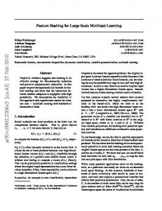
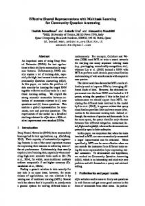
4. Experiments In this section we analyze the statistical performance of FETR as well as the efficiency of the proposed coordinate minimization algorithm for solving the underlying multi-convex optimization problem. 4.1 Convergence Analysis We first investigate the efficiency and scalability of the three different algorithms for minimizing w.r.t. W on synthetic data sets. To this end, for each experiment, we generate a synthetic data set which consists of n = 104 instances that are shared among all the tasks. All the instances are randomly sampled uniformly from [0, 1]d . We gradually increase the dimension of features, d, and the number of tasks, m to test scalability. The first algorithm implements the closed form solution (21) by explicitly computing the md × md tensor product matrix and then solving the linear system. The second one is the proposed gradient descent, whose stop condition is met when either the norm of the gradient is less than 0.01 or the algorithm has looped more than 50 iterations. The last one uses the Bartels-Stewart algorithm to solve the equivalent Sylvester equation to compute W . We use open source toolkit scipy whose backend implementation uses highly optimized Fortran code. For all the synthetic experiments we set l = 0.01 and u = 100, which corresponds to a condition number of 104 . We fix the coefficients η = 1.0 and ρ = 1.0 since they will not affect the convergence speed. The experimental results are shown in Fig. 1. As expected, the closed form solution does not scale to problems of even moderate size due to its large memory requirement. In practice the Bartels-Stewart algorithm is about one order of magnitude faster than the gradient descent method when either m or d is large (hundreds of features or hundreds of tasks). It is also worth pointing out here that the Bartels-Stewart algorithm is the most numerically stable algorithm among the three based on our observations. Hence in the following experiments where the Bartels-Stewart solver can be applied we will use it, while in the case where it cannot be applied, we will use the gradient descent method. We now compare our proposed coordinate minimization algorithm with an off-the-shelf projected gradient method to solve the optimization problem (7). Specifically, the projected gradient method updates W, Σ1 and Σ2 based on the gradient direction in each iteration and then projects Σ1 and Σ2 into the corresponding feasible regions. In this experiment we set the number of instances to be 104 , the dimension of feature vectors to be 104 and the number of tasks to be 10. All the instances are shared among all the tasks, so that the Sylvester solver is used to optimize W in coordinate minimization. We repeat the experiments 10 times and report the log function values versus the time used by these two algorithms; see Fig. 2. We use a desktop with twelve i7-6850K CPU cores to conduct this experiment. It is clear from this synthetic experiment that our proposed algorithm not only converges much faster than projected gradient descent, but also achieves better results. 4.2 Synthetic Toy Problem Before we proceed to do experiments on real-world data sets, we generate a toy data set and conduct a synthetic experiment to show that the proposed model can indeed learn the relationships between task vectors and feature vectors simultaneously. We randomly generate 10 data points uniformly from the range [0, 100]2 . We consider the following three regression tasks: y1 = 10x1 + 10x2 + 10, 11

H AN Z HAO , OTILIA S TRETCU , R ENATO N EGRINHO , A LEX S MOLA , G EOFF G ORDON

Closed Gradient Sylvester

Closed Gradient Sylvester

Closed Gradient Sylvester

Closed Gradient Sylvester

Closed Gradient Sylvester

Closed Gradient Sylvester

Closed Gradient Sylvester

Closed Gradient Sylvester

d = 1000

d = 100

d = 10

Closed Gradient Sylvester

m = 10

m = 100

m = 1000

Figure 1: Each experiment is repeated 10 times. We plot the mean run time (seconds) and the standard deviation for each algorithm under each experimental configuration. Closed form solution does not scale when md ≥ 104 . y2 = 0, and y3 = −8x1 − 8x2 − 8. The outputs of those regression functions are corrupted by Gaussian noise with mean 0 and variance 1. The true weight matrix is given by   10 0 −8 ∗ W = 10 0 −8 For this problem, the first row of W ∗ corresponds to the weight vector of the feature x1 across the tasks and the second row corresponds to the weight vector of x2 . Each column represents a task vector. Hence we expect that the correlation between x1 and x2 is 1.0, and we also expect that the 12

E FFICIENT M ULTI - TASK F EATURE AND R ELATIONSHIP L EARNING

Coordinate Minimization v.s. Projected Gradient Descent

16

Coordinate minimization Projected gradient descent 14

log function value

12

10

8

6

4

0

10

20

30

40

50

Time (seconds)

Figure 2: The convergence speed of coordinate minimization versus projected gradient descent. All the experiments are repeated for 10 times. correlation between the first and the third task to be -1.0 while the correlations for the other two pairs of tasks are 0.0. We apply FETR to this problem, setting η, ρ = 10−3 , l = 10−3 and u = 103 . After the algorithm converges, the estimated regression functions are yˆ1 = 10.00x1 + 9.99x2 + 9.43, yˆ2 = 0.00 and yˆ3 = −7.99x1 − 8.01x2 − 7.56, with the following feature and task correlation matrices (after normalization):     1.00 0.00 −1.01 1.00 0.99 , Ω2 =  0.00 1.00 0.00  Ω1 = 0.99 1.00 −1.01 0.00 1.00 This synthetic experiment shows that both the learned feature correlation matrix and task correlation matrix conform to our expectation, demonstrating the effectiveness of FETR on this synthetic problem. 4.3 Robot Inverse Dynamics We evaluate FETR against other multi-task learning algorithms on the inverse dynamics problem for a seven degree-of-freedom (DOF) SARCOS anthropomorphic robot arm.2 The goal of this task is to map from a 21-dimensional input space (7 joint positions, 7 joint velocities, 7 joint accelerations) to the corresponding 7 joint torques. Hence there are 7 tasks and the inputs are shared among all the tasks. The training set and test set contain 44,484 and 4,449 examples, respectively. We further partition the training set into a development set and a validation set, which contain 31,138 and 13,346 instances. We use the validation set to do the model selection. Specifically, we train multiple models on the development set with different configurations of hyperparameters ranging 2. http://www.gaussianprocess.org/gpml/data/

13

H AN Z HAO , OTILIA S TRETCU , R ENATO N EGRINHO , A LEX S MOLA , G EOFF G ORDON

0.6 STL MTFL MTRL FETR

0.5 0.4

log nMSE

0.3 0.2 0.1 0.0 0.1 0.2

50

100

150

200

500

1000

2000

5000

10000

Training size

Figure 3: The log total normalized mean squared error of 7 tasks on the SARCOS data set. The x-axis represents the size of the training data set. from η = {10−5 , . . . , 102 } and ρ = {10−5 , . . . , 102 }, and for each model we select the one with the best mean-squared error (MSE) on the validation set. In all the experiments we fix l = 10−3 and u = 103 as we observe the results are not very sensitive to these hyperparameters. We compare FETR with multi-task feature learning (Evgeniou and Pontil, 2007) (MTFL) and multitask relationship learning (Zhang and Yeung, 2010a) (MTRL), which can be treated as two different special cases of our model. To have a more controlled, fair comparison between all the methods, we implement both MTFL and MTRL, and use the same experimental setting, including model selection, as FETR. For each task, we use ridge regression as our baseline model, and denote it as single task learning (STL). For each method, the best model on the validation set is used to do prediction, and we report its MSE score on the test set for each task. The smaller the MSE score, the better the predictive result. The results are summarized in Table 1. As expected, when the size of the training data set is large, all the multi-task learning methods perform at least as well as the baseline STL method. Table 1: Mean squared error of different methods on the SARCOS data. Each column corresponds to one task. Method STL MTFL MTRL FETR

1st DOF 31.40 31.41 31.09 31.08

2nd DOF 22.90 22.91 22.69 22.68

3rd DOF 9.13 9.13 9.08 9.08

4th DOF 10.30 10.33 9.74 9.73

5th DOF 0.14 0.14 0.14 0.13

6th DOF 0.84 0.83 0.83 0.83

7th DOF 0.46 0.45 0.44 0.43

Among the three multi-task learning methods, FETR achieves the lowest test set mean square error. FETR can learn both covariance matrices over features and tasks simultaneously, while the other two methods can only estimate one of them. To illustrate this, we show the covariance matrices 14

E FFICIENT M ULTI - TASK F EATURE AND R ELATIONSHIP L EARNING

estimated by MTFL, MTRL and FETR in the appendix. We also test the performance of all four methods as the size of the training set increases. In order to summarize an overall performance score for better visualization, we use the log total normalized mean squared error of seven tasks on the original test data set, that is, the log sum of the mean squared error divided by the variance of the ground truth. This helps to illustrate the advantages of multi-task learning methods over single task learning as the data set gets larger. For each training set size, we repeat the experiments 10 times, by randomly sampling a subset of the corresponding size from the whole training set. We depict the mean log nMSE of all four methods as well as the standard deviation in Fig. 3. We also plot the covariance matrices estimated by MTFL, MTRL and FETR to compare the correlation structures found by these algorithms; see Fig. 4. It is worth mentioning that not only does FETR learn both correlation matrices, but it also detects more correlations between features than MTFL. For example, the task correlation matrix learned by FETR exhibits a block diagonal structure, meaning that the weight vectors for the first 4 tasks are roughly uncorrelated. Such pattern is not shown in the task correlation matrix learned by MTRL. On the other hand, FETR detects more correlations among features than MTFL, as shown in Fig. 4.

MTRL task correlation matrix 1

2

1

MTFL feature correlation matrix

0.8

2

6

5

4

3

0.8

21 20 19 18 17 16 15 14 13 12 11 10 9

3

0.4

8

7

0.4

0.0

5

4

0.0

0.4 6

0.4

0.8 7

0.8

1

2

3

4

5

6

7

8

9 10 11 12 13 14 15 16 17 18 19 20 21

1

2

3

4

5

6

7

FETR task correlation matrix 1

2

1

FETR feature correlation matrix

0.8

2

6

5

4

3

0.8

21 20 19 18 17 16 15 14 13 12 11 10 9

3

0.4

8

7

0.4

0.0

5

4

0.0

0.4 6

0.4

0.8 7

0.8

1

2

3

4

5

6

7

8

9 10 11 12 13 14 15 16 17 18 19 20 21

1

2

3

4

5

6

7

Figure 4: Correlation matrices of feature vectors and task vectors learned by MTFL, MTRL and FETR.

15

H AN Z HAO , OTILIA S TRETCU , R ENATO N EGRINHO , A LEX S MOLA , G EOFF G ORDON

5. Related Work Multi-task learning is an area of active research in machine learning and has received a lot of attention in the past years (Thrun, 1996b; Caruana, 1997; Yu et al., 2005; Bonilla et al., 2007a,b; Argyriou et al., 2007, 2008; Zhang and Yeung, 2010a). Research on multi-task learning has been carried in several strands. Early work focuses on sharing knowledge in separate tasks by sharing hidden representations, for example, hidden layer of units in neural networks (Caruana, 1997). Another stream of works constructs a Gaussian process prior over the regression functions in different tasks and the transfer of knowledge between tasks is enforced by the structure of the covariance functions/kernels of the Gaussian process prior. Bonilla et al. (2007a) presents a kernel multi-task learning approach with Gaussian process prior where task-specific features are assumed to be available. They concatenate the feature for input instance with the task feature and then define a kernel covariance function over the regression functions among different tasks. The learning is reduced to inferring the hyperparameters of the kernel function by maximizing the marginal log-likelihood of the instances by either EM or gradient ascent. This approach essentially decomposes the joint kernel function over regression functions into two separate kernels: one measures the similarity among tasks and the other measures the similarity among instances. A closely related approach in this strand is to consider a nonparametric kernel matrix over the tasks rather than a parametrized kernel function (Bonilla et al., 2007b). However, the kernel over input instances is still restricted to be parametrized in order to avoid the expensive computation of semidefinite programming over input features. In contrast, FETR optimizes both of the feature and task covariance matrices directly without assumption about their parametrized forms. Argyriou et al. (2008) and (Zhang and Yeung, 2010a) develop MTFL and MTRL, which can be viewed as convex frameworks of learning the feature and the task-relatedness covariance matrices, respectively. Both MTFL and MTRL are essentially convex regularization methods that exploit the feature and task relatedness by imposing trace constraints on W after proper transformations. Covariance matrices in MTFL and MTRL are not restricted to have specific parametrized forms, and from this perspective, (Evgeniou et al., 2005; Evgeniou and Pontil, 2004; Kato et al., 2008) can be understood as special cases of MTFL and MTRL where the covariance matrices are constrained to be (weighted) graph Laplacians. However, in MTFL only the feature covariance matrix is being optimized and the task-relatedness covariance matrix is assumed to be the identity, while in MTRL only the task-relatedness covariance matrix is being optimized and the feature covariance matrix is, again, assumed to be the identity. We take inspiration from these two previous works and propose a general regularization framework, FETR, that models and optimizes both task and feature relationships directly. It is worth emphasizing here that both MTFL and MTRL can be treated as special cases of FETR where one of the two covariance matrices are assumed to be the identity, which corresponds to left/right spherical matrix normal distributions. The objective function of FETR is not convex, but multi-convex. Efficient coordinate-wise minimization algorithm with closed form solutions for each subproblem is designed to tackle the multi-convex objective in FETR. Perhaps the most related work to FETR is Zhang and Schneider (2010). Both that work and our approach consider a multi-task learning framework where both the task and feature covariance matrices are inferred from data. However, while the authors make a sparsity assumption on the two covariance matrices, our approach is more general in the sense that we are free of this assumption. Secondly and more importantly, while in that work the optimization w.r.t the two covariance matrices employs an iterative method (either proximal method or coordinate descent) to approximate 16

E FFICIENT M ULTI - TASK F EATURE AND R ELATIONSHIP L EARNING

the optimal solution, we obtain an efficient, non-iterative solution by reduction to a graph matching problem. Note that in order to optimize the covariance matrix using our method, one SVD is enough, while in Zhang et al. each iteration requires an SVD. This makes our approach computationally more efficient than the one used in Zhang and Schneider (2010), and statistically our approach makes less assumption than the framework proposed in Zhang and Schneider (2010).

6. Discussion and future work We develop a multi-convex framework for multi-task learning that improves predictions by learning relationships both between tasks and between features. Our framework is a generalization of related approaches in multi-task learning, that either learn task relationships, or feature relationships. We develop a multi-convex formulation of the problem, as well as an algorithm for block coordinatewise minimization. By using the theory of doubly stochastic matrices, we are able to reduce the underlying matrix optimization subproblem into a minimum weight perfect matching problem on a complete bipartite graph, and solve it in closed form. Our method is orders of magnitude faster than an off-the-shelf projected gradient descent method, and it shows improved performance on synthetic datasets as well as on a real-world dataset for robotic modeling. While the current paper discusses our approach in the context of linear regression, it can be extended to other types of prediction tasks, such as logistic regression, linear SVM, etc.

References A. Argyriou, M. Pontil, Y. Ying, and C. A. Micchelli. A spectral regularization framework for multi-task structure learning. In Advances in neural information processing systems, 2007. A. Argyriou, T. Evgeniou, and M. Pontil. Convex multi-task feature learning. Machine Learning, 73(3):243–272, 2008. R. H. Bartels and G. Stewart. Solution of the matrix equation AX+ XB= C [F4]. Communications of the ACM, 15(9):820–826, 1972. D. Bertsimas and J. N. Tsitsiklis. Introduction to linear optimization, volume 6. Athena Scientific Belmont, MA, 1997. R. Bhatia and P. Rosenthal. How and why to solve the operator equation ax- xb= y. Bulletin of the London Mathematical Society, 29(01):1–21, 1997. E. V. Bonilla, F. V. Agakov, and C. Williams. Kernel multi-task learning using task-specific features. In International Conference on Artificial Intelligence and Statistics, pages 43–50, 2007a. E. V. Bonilla, K. M. Chai, and C. Williams. Multi-task gaussian process prediction. In Advances in neural information processing systems, pages 153–160, 2007b. S. Boyd and L. Vandenberghe. Convex optimization. 2004. B. P. Carlin and T. A. Louis. Bayes and empirical bayes methods for data analysis. Statistics and Computing, 7(2):153–154, 1997. R. Caruana. Multitask learning. Machine learning, 28(1):41–75, 1997. 17

H AN Z HAO , OTILIA S TRETCU , R ENATO N EGRINHO , A LEX S MOLA , G EOFF G ORDON

F. Dufoss´e and B. Uc¸ar. Notes on birkhoff–von neumann decomposition of doubly stochastic matrices. Linear Algebra and its Applications, 497:108–115, 2016. A. Evgeniou and M. Pontil. Multi-task feature learning. Advances in neural information processing systems, 19:41, 2007. T. Evgeniou and M. Pontil. Regularized multi–task learning. In Proceedings of the tenth ACM SIGKDD international conference on Knowledge discovery and data mining, pages 109–117. ACM, 2004. T. Evgeniou, C. A. Micchelli, and M. Pontil. Learning multiple tasks with kernel methods. In Journal of Machine Learning Research, pages 615–637, 2005. J. Gorski, F. Pfeuffer, and K. Klamroth. Biconvex sets and optimization with biconvex functions: a survey and extensions. Mathematical Methods of Operations Research, 2007. A. K. Gupta and D. K. Nagar. Matrix variate distributions, volume 104. CRC Press, 1999. T. Kato, H. Kashima, M. Sugiyama, and K. Asai. Multi-task learning via conic programming. In Advances in Neural Information Processing Systems, pages 737–744, 2008. Y. Li, X. Tian, T. Liu, and D. Tao. Multi-task model and feature joint learning. In Proceedings of the 24th International Conference on Artificial Intelligence, pages 3643–3649. AAAI Press, 2015. J. Liu, S. Ji, and J. Ye. Multi-task feature learning via efficient l 2, 1-norm minimization. In Proceedings of the twenty-fifth conference on uncertainty in artificial intelligence, pages 339– 348. AUAI Press, 2009. Y. Nesterov. Introductory lectures on convex optimization: A basic course, volume 87. Springer Science & Business Media, 2013. J. R. Shewchuk et al. An introduction to the conjugate gradient method without the agonizing pain, 1994. S. Thrun. Explanation-based neural network learning. In Explanation-Based Neural Network Learning, pages 19–48. Springer, 1996a. S. Thrun. Is earning the n-th thing any easier than learning the first? Advances in neural information processing systems, pages 640–646, 1996b. Y. Xu and W. Yin. A block coordinate descent method for regularized multiconvex optimization with applications to nonnegative tensor factorization and completion. SIAM Journal on imaging sciences, 2013. K. Yu, V. Tresp, and A. Schwaighofer. Learning gaussian processes from multiple tasks. In Proceedings of the 22nd international conference on Machine learning, pages 1012–1019. ACM, 2005. Y. Zhang and J. G. Schneider. Learning multiple tasks with a sparse matrix-normal penalty. In Advances in Neural Information Processing Systems, pages 2550–2558, 2010. 18

E FFICIENT M ULTI - TASK F EATURE AND R ELATIONSHIP L EARNING

Y. Zhang and D.-Y. Yeung. A convex formulation for learning task relationships in multi-task learning. 2010a. Y. Zhang and D.-Y. Yeung. Multi-task learning using generalized t process. In AISTATS, pages 964–971, 2010b.

19

H AN Z HAO , OTILIA S TRETCU , R ENATO N EGRINHO , A LEX S MOLA , G EOFF G ORDON

Appendix A. Proofs A.1 Proofs of Claim 3.1 Claim 3.1. The objective function in (6) is multi-convex. Proof. First, it is straightforward to check that the constraint set lId  Σ1  uId and lIm  Σ2  uIm are convex. For any fixed Σ1 and Σ2 , the objective function in terms of W can be expressed as   ni m X X  (y j − wiT xj )2 + η||wi ||22  + ρtr(Σ1 W Σ2 W T ) i i i=1

j=1

P i The first term decomposes over tasks and for each task vector wi , nj=1 (yij − wiT xji )2 + η||wi ||22 is a quadratic function for each wi , so the summation is also convex in W . Since Σ1 ∈ Sd+ and Σ2 ∈ Sm + , we can further rewrite the second term above as 1/2

1/2

1/2

1/2

1/2

1/2

ρtr(Σ1 W Σ2 W T ) = ρtr((Σ1 W Σ2 )(Σ1 W Σ2 )T ) = ρ||Σ1 W Σ2 ||2F 1/2

1/2

This is the Frobenius norm of the matrix Σ1 W Σ2 , which is a linear transformation of W when both Σ1 and Σ2 are fixed, hence this is also a convex function of W . Overall the objective function with respect to W when both Ω1 and Ω2 are fixed is convex. For any fixed W and Σ2 , consider the objective function with respect to Σ1 : −ρm log |Σ1 | + ρtr(Σ1 C) where C = W Σ2 W T is a constant matrix. Since log |Σ1 | is concave in Σ1 and tr(Σ1 C) is a linear function of Σ1 , it directly follows that −ρm log |Σ1 | + ρtr(Σ1 C) is a convex function of Σ1 . A similar argument can be applied to Σ2 as well.  A.2 Proof of Claim 3.2 Claim 3.2. (8) can be solved in closed form in O(m3 d3 + mnd2 ) time; the optimal vec(W ∗ ) has the following form: Im ⊗ (X T X) + ηImd + ρΣ2 ⊗ Σ1


−1

vec(X T Y )

(10)

To prove this claim, we need the following facts about tensor product: Fact A.1. Let A be a matrix. Then ||A||F = ||vec(A)||2 . Fact A.2. Let A ∈ Rm1 ×n1 , B ∈ Rn1 ×n2 and C ∈ Rn2 ×m2 . Then vec(ABC) = (C T ⊗ A)vec(B). Fact A.3. Let S1 ∈ Rm1 ×n1 , S2 ∈ Rn1 ×p1 and T1 ∈ Rm2 ×n2 , T2 ∈ Rn2 ×p2 . Then (S1 ⊗ S2 )(T1 ⊗ T2 ) = (S1 S2 ) ⊗ (T1 T2 ). Fact A.4. Let A ∈ Rn×n and B ∈ Rm×m . Let {µ1 , . . . , µn } be the spectrum of A and {ν1 , . . . , νm } be the spectrum of B. Then the spectrum of A ⊗ B is {µi νj : 1 ≤ i ≤ n, 1 ≤ j ≤ m}. we can show the following result by transforming W into its isomorphic counterpart: 20

E FFICIENT M ULTI - TASK F EATURE AND R ELATIONSHIP L EARNING

Proof. 1/2

1/2

||Y − XW ||2F + η||W ||2F + ρ||Σ1 W Σ2 ||2F

1/2

1/2

= ||vec(Y − XW )||22 + η||vec(W )||22 + ρ||vec(Σ1 W Σ2 )||22

(By Fact A.1)

= ||vec(Y ) − (Im ⊗ +  = vec(W )T (Im ⊗ X)T (Im ⊗ X) + ηImd +

(By Fact A.2)

X)vec(W )||22

1/2 1/2 + ρ||(Σ2 ⊗ Σ1 )vec(W )||22  1/2 1/2 1/2 1/2 ρ(Σ2 ⊗ Σ1 )T (Σ2 ⊗ Σ1 ) vec(W )

η||vec(W )||22

− 2vec(W )T (Im ⊗ X T )vec(Y ) + vec(Y )T vec(Y )
= vec(W )T (Im ⊗ X T X) + ηImd + ρ(Σ2 ⊗ Σ1 ) vec(W ) − 2vec(W )T (Im ⊗ X T )vec(Y ) + vec(Y )T vec(Y )

(By Fact A.3)

The last equation above is a quadratic function of vec(W ), from which we can read off that the optimal solution W ∗ should satisfy:
−1 vec(W ∗ ) = Im ⊗ (X T X) + ηImd + ρΣ2 ⊗ Σ1 vec(X T Y ) (21) W ∗ can then be obtained simply by reformatting vec(W ∗ ) into a d × m matrix. The computational bottleneck in the above procedure is in solving an md × md system of equations, which scales as O(m3 d3 ) if no further structure is available. The overall computational complexity is O(m3 d3 + mnd2 ).  A.3 Proof of Thm. 3.1 To analyze the convergence rate of gradient descent in this case, we start by bounding the smallest and largest eigenvalue of the quadratic system shown in Eq. 21. Lemma A.1 (Weyl’s inequality). Let A, B and C be n-by-n Hermitian matrices, and C = A + B. Let a1 ≥ · · · ≥ an , b1 ≥ · · · ≥ bn and c1 ≥ · · · ≥ cn be the eigenvalues of A, B and C respectively. Then the following inequalities hold for r + s − 1 ≤ i ≤ j + k − n, ∀i = 1, . . . , n: aj + bk ≤ ci ≤ ar + bs Let λk (A) be the k-th largest eigenvalue of matrix A. Lemma A.2. If Σ1 and Σ2 are feasible in (7), then λ1 (Im ⊗ (X T X) + ηImd + ρΣ2 ⊗ Σ1 ) ≤ λ1 (X T X) + η + ρu2 λmd (Im ⊗ (X T X) + ηImd + ρΣ2 ⊗ Σ1 ) ≥ λd (X T X) + η + ρl2 Proof. By Weyl’s inequality, setting r = s = i = 1, we have c1 ≤ a1 + b1 . Set j = k = i = n, we have cn ≥ an + bn . We can bound the largest and smallest eigenvalues of Im ⊗ (X T X) + ηImd + ρΣ2 ⊗ Σ1 as follows: λ1 (Im ⊗ (X T X) + ηImd + ρΣ2 ⊗ Σ1 )

≤ λ1 (Im ⊗ (X T X)) + λ1 (ηImd ) + λ1 (ρΣ2 ⊗ Σ1 )

= λ1 (Im )λ1 (X T X) + η + ρλ1 (Σ1 )λ1 (Σ2 ) T

2

≤ λ1 (X X) + η + ρu

(By Weyl’s inequality) (By Fact A.4) (By the feasibility assumption)

21

H AN Z HAO , OTILIA S TRETCU , R ENATO N EGRINHO , A LEX S MOLA , G EOFF G ORDON

and λmd (Im ⊗ (X T X) + ηImd + ρΣ2 ⊗ Σ1 )

≥ λmd (Im ⊗ (X T X)) + λmd (ηImd ) + λmd (ρΣ2 ⊗ Σ1 ) T

(By Weyl’s inequality)

= λm (Im )λd (X X) + η + ρλm (Σ1 )λd (Σ2 )

(By Fact A.4)

≥ λd (X T X) + η + ρl2

(By the feasibility assumption) 

We will first prove the following two lemmas using the fact that the spectral norm of the Hessian matrix ∇2 h(W ) is bounded. Lemma A.3. Let f (W ) : Rd×m 7→ R be a twice differentiable function with λ1 (∇2 f (W )) ≤ L. L > 0 is a constant. The minimum value of f (W ) can be achieved. Let W ∗ = arg minW f (W ), then 1 ||∇f (W )||2F f (W ∗ ) ≤ f (W ) − 2L Proof. Since f (W ) is twice differentiable with λ1 (∇2 f (W )) ≤ L, by the Lagrangian mean value f , we can find a value 0 < t(W, W f ) < 1, such that theorem, ∀W, W f ) = f (W ) + tr(∇f (W )T (W f − W )) + 1 vec(W f − W )T ∇2 f (tW + (1 − t)W f )vec(W f − W) f (W 2 f − W )) + L ||W f − W ||2F ≤ f (W ) + tr(∇f (W )T (W 2 Since W ∗ achieves the minimum value of f (W ), we can use the above result to obtain: f) f (W ∗ ) = inf f (W f W

f − W )) + ≤ inf f (W ) + tr(∇f (W )T (W f W

= f (W ) −

L f ||W − W ||2F 2

1 ||∇f (W )||2F 2L

where the last equation comes from the fact that the minimum of a quadratic function with respect f can be achieved at W f = W − 1 ∇f (W ).  to W L Lemma A.4. Let f (W ) : Rd×m 7→ R be a convex, twice differentiable function with λ1 (∇2 f (W )) ≤ L. L > 0 is a constant, then ∀W1 , W2 :
1 tr (∇f (W1 ) − ∇f (W2 ))T (W1 − W2 ) ≥ ||∇f (W1 ) − ∇f (W2 )||2F L Proof. For all W1 , W2 , we can construct the following two functions:
fW1 (Z) = f (Z) − tr ∇f (W1 )T Z ,

fW2 (Z) = f (Z) − tr ∇f (W2 )T Z 22




E FFICIENT M ULTI - TASK F EATURE AND R ELATIONSHIP L EARNING

Since f (W ) is a convex, twice differentiable function with respect to W , it follows that both fW1 (Z) and fW2 (Z) are convex, twice differentiable functions with respect to Z. The first-order optimality condition of convex functions gives the following conditions to hold for Z which achieves the optimality: ∇fW2 (Z) = ∇f (Z) − f (W2 ) = 0

∇fW1 (Z) = ∇f (Z) − ∇f (W1 ) = 0,

Plug in W1 and W2 into the above optimality conditions respectively. From the first-order optimality condition we know that W1 and W2 achieves the optimal solutions of fW1 (Z) and fW2 (Z), respectively. Now applying Lemma A.3 to fW1 (Z) and fW2 (Z), we have: (W2 ) − tr ∇f (W1 )T W2





− (W1 ) − tr ∇f (W1 )T W1





≥

1 ||∇f (W1 ) − ∇f (W2 )||2F 2L

(W1 ) − tr ∇f (W2 )T W1





− (W2 ) − tr ∇f (W2 )T W2





≥

1 ||∇f (W1 ) − ∇f (W2 )||2F 2L

Adding the above two equations leads to
1 tr (∇f (W1 ) − ∇f (W2 ))T (W1 − W2 ) ≥ ||∇f (W1 ) − ∇f (W2 )||2F L  We can now proceed to show Thm. 3.1. −λl 2 Theorem 3.1. Let λl = λd (X T X) + η + ρl2 , λu = λ1 (X T X) + η + ρu2 and γ = ( λλuu +λ ) . l Choose 0 < t ≤ 2/(λu + λl ). For all ε > 0, gradient descent with step size t converges to the optimal solution within O(log1/γ (1/ε)) steps.

Proof. Define function g(W ) as follows: g(W ) = h(W ) −

λl ||W ||2F 2

Since we have already bounded that λmd (∇2 h(W )) ≥ λl , it follows that g(W ) is a convex function and furthermore λ1 (∇2 g(W )) ≤ λu − λl . Applying Lemma A.4 to g, ∀W1 , W2 ∈ Rd×m , we have:
tr (∇g(W1 ) − ∇g(W2 ))T (W1 − W2 ) ≥

1 ||∇g(W1 ) − ∇g(W2 )||2F λu − λl

Plug in ∇g(W ) = ∇h(W )−λl W into the above inequality and after some algebraic manipulations, we have:
tr (∇h(W1 ) − ∇h(W2 ))T (W1 − W2 ) ≥

1 λu λl ||∇h(W1 )−∇h(W2 )||2F + ||W1 −W2 ||2F λu + λl λu + λl (22) 23

H AN Z HAO , OTILIA S TRETCU , R ENATO N EGRINHO , A LEX S MOLA , G EOFF G ORDON

Let W ∗ = arg minW h(W ). Within each iteration of Alg. 3, we have the update formula as W + = W − t∇h(W ), we can bound ||W + − W ∗ ||2F as follows ||W + − W ∗ ||2F = ||W − W ∗ − t∇h(W )||2F


= ||W − W ∗ ||2F + t2 ||∇h(W )||2F − 2ttr (W − W ∗ )T ∇h(W ) 2 λu λl )||W − W ∗ ||2F + t(t − )||∇h(W )||2F (By inequality 22) ≤ (1 − 2t λu + λl λu + λl λu λl ≤ (1 − 2t )||W − W ∗ ||2F (For 0 < t ≤ 2/(λu + λl )) λu + λl

Apply the above inequality recursively for T times, we have ||W (T ) − W ∗ ||2F ≤ γ T ||W (0) − W ∗ ||2F λl . For t = 2/(λu + λl ), we have where γ = 1 − 2t λλuu+λ l

γ = 1 − 4λu λu /(λl + λu )2 =



λu − λl λu + λl

2

Now pick ∀ε > 0, setting the upper bound γ T ||W (0) − W ∗ ||2F ≤ ε and solve for T , we have T ≥ log1/γ (C/ε) = O(log1/γ (1/ε)) where C = ||W (0) − W ∗ ||2F is a constant.



The pseudocode of the gradient descent is shown in Alg. 3. Algorithm 3 Gradient descent with fixed step-size. Input: Initial W , X, Y and approximation accuracy ε. 1: λu ← λ1 (X T X) + η + ρu2 . 2: λl ← λd (X T X) + η + ρl2 . 3: Step size t ← 2/(λl + λu ). 4: while ||∇h(W )||F > ε do
5: W ← W − t X T (Y − XW ) + ηW + ρΣ1 W Σ2 . 6: end while

A.4 Proof of Lemma 3.1 Lemma 3.1. There exists an optimal solution P to the optimization problem (18) that is a d × d permutation matrix. Proof. Note that the optimization problem (18) in terms of P is a linear program with the Birkhoff polytope being the feasible region. It follows from Thm. 3.2 and Thm. 3.3 that at least one optimal solution P is an d × d permutation matrix.  24

E FFICIENT M ULTI - TASK F EATURE AND R ELATIONSHIP L EARNING

A.5 Proof of Thm. 3.4 Theorem 3.4. The minimum value of (18) is equal to the minimum weight of a perfect matching on G = (Vλ , Vν , E, w). Furthermore, the optimal solution P of (18) can be constructed from the minimum-weight perfect matching M on G. Proof. By Lemma 3.1, the optimal value is achieved when P is a permutation matrix. Given a permutation matrix P , we can understand P as a bijective mapping from the index of rows to the index of columns. Specifically, construct a permutation πP : [d] → [d] from P as follows. For each row index i ∈ [d], πP (i) = j iff Pij = 1. It follows that πP is a permutation of [d] since P is assumed to be a permutation matrix. The objective function in (18) can be written in terms of πP as T

λ Pν =

d X

λi νπP (i)

i=1

which is exactly the weight of the perfect matching on G(Vλ , Vν , E, w) given by πP : w(πP ) = w({(i, πP (i)) : 1 ≤ i ≤ d}) =

d X

λi νπP (i)

i=1

Similarly, in the other direction, given any perfect matching π : [d] → [d] on the bipartite graph G(Vλ , Vν , E, w), we can construct a corresponding permutation matrix Pπ : Pπ,ij = 1 iff π(i) = j, otherwise 0. Since π is a perfect matching, the constructed Pπ is guaranteed to be a permutation matrix. Hence the problem of finding the optimal value of (18) is equivalent to finding the minimum weight perfect matching on the constructed bipartite graph G(Vλ , Vν , E, w). Note that the above constructive process also shows how to recover the optimal permutation matrix Pπ∗ from the minimum weight perfect matching π ∗ .  A.6 Proof of Thm. 3.5 Note that λ = (λ1 , . . . , λd ) and ν = (ν1 , . . . , νd ) are assumed to satisfy λ1 ≥ · · · ≥ λd and ν1 ≤ · · · ≤ νd . To make the discussion more clear, we first make the following definition of an inverse pair. Definition A.1 (Inverse pair). Given a perfect match π of G(Vλ , Vν , E, w), (λi , λj , νk , νl ) is called an inverse pair if i ≤ j, k ≤ l and (vλi , vνl ) ∈ π, (vλj , vνk ) ∈ π. Lemma A.5. Given a perfect match π of G(Vλ , Vν , E, w) and assuming π contains an inverse pair (λi , λj , νk , νl ). Construct π 0 = π\{(vλi , vνl ), (vλj , vνk )} ∪ {((vλi , vνk ), (vλj , vνl )}. Then w(π 0 ) ≤ w(π). Proof. Let us compare the weights of π and π 0 . Note that since i ≤ j, k ≤ l, we have λi ≥ λj and νk ≤ νl . w(π 0 ) − w(π) = (λi νk + λj νl ) − (λi νl + λj νk ) = (λi − λj )(νk − νl )

≤0

25

H AN Z HAO , OTILIA S TRETCU , R ENATO N EGRINHO , A LEX S MOLA , G EOFF G ORDON

λi

λj

λi

λj

νk

νl

νk

νl

Figure 5: Re-matching an inverse pair (λi , λj , νk , νl ) = {(vλi , vνl ), (vλj , vνk )} on the left side to a match with smaller weight {(vλi , vνk ), (vλj , vνl )}. Red color is used to highlight edges in the perfect matching. Intuitively, this lemma says that we can always decrease the weight of a perfect matching by rematching an inverse pair. Fig. 5 illustrates this process. It is worth emphasizing here that the above re-matching process only involves four nodes, i.e., vλi , vνl , vλj and vνk . In other words, the other parts of the matching stay unaffected.  Using Lemma A.5, we are now ready to prove Thm. 3.5: Theorem 3.5. Let λ = (λ1 , . . . , λd ) and ν = (ν1 , . . . , νd ) with λ1 ≥ · · · ≥ λd and ν1 ≤ · · · ≤ νd . The minimum-weight perfect matching on G is π ∗ = {(vλi , vνi ) : 1 ≤ i ≤ d} with the minimum P weight w(π ∗ ) = di=1 λi νi . Proof. We will prove by induction. • Base case. The base case is d = 2. In this case there are only two valid perfect matchings, i.e., {(vλ1 , vν1 ), (vλ2 , vν2 )} or {(vλ1 , vν2 ), (vλ2 , vν1 )}. Note that the second perfect matching {(vλ1 , vν2 ), (vλ2 , vν1 )} is an inverse pair. Hence by Lemma A.5, w({(vλ1 , vν1 ), (vλ2 , vν2 )}) = λ1 ν1 + λ2 ν2 ≤ λ1 ν2 + λ2 ν1 = w({(vλ1 , vν2 ), (vλ2 , vν1 )}). • Induction step. Assume Thm. 3.5 holds for d = n. Consider the case when d = n + 1. Start from any perfect matching π. Check the matches of node vλn+1 and vνn+1 . Here we have two subcases to discuss: – If vλn+1 is matched to vνn+1 in π. Then we can remove nodes vλn+1 and vνn+1 from current graph, and this reduces to the case when n = d. By induction P assumption, the minimum weight perfect matching onP the new graph is given by P ni=1 λi νi , so the minimum weight on the original graph is ni=1 λi νi + λn+1 νn+1 = n+1 i=1 λi νi . – If vλn+1 is not matched to vνn+1 in π. Let vνj be the match of vλn+1 and vλi be the match of vνn+1 , where i 6= n + 1 and j 6= n + 1. In this case we have i < n + 1 and j < n + 1, so (λi , λn+1 , νj , νn+1 ) forms an inverse pair by definition. By Lemma A.5, we can first re-match vλn+1 to vνn+1 and vλi to vνj to construct a new match π 0 with w(π 0 ) ≤ w(π). In the new matching π 0 we have the property that vλn+1 is matched to vνn+1 , and this becomes the above case that we have already analyzed, so we still have P the minimum weight perfect matching to be n+1 i=1 λi νi . 26

E FFICIENT M ULTI - TASK F EATURE AND R ELATIONSHIP L EARNING

Intuitively, as shown in Fig. 5, an inverse pair corresponds to a cross in the matching graph. The above inductive proof basically works from right to left to recursively remove inverse pairs (crosses) from the matching graph. Each re-matching step in the proof will decrease the number of inverse pairs at least by one. The whole process stops until there is no inverse pair in the current perfect matching. Since the total number of possible inverse pairs, the above process can stop in finite steps. We illustrate the process of removing inverse pairs in Fig. 6.  λ1

λ2

···

λd

λ1

λ2

···

λd

λ1

λ2

···

λd

ν1

ν2

···

νd

ν1

ν2

···

νd

ν1

ν2

···

νd

Figure 6: The inductive proof works by recursively removing inverse pairs from the right side of the graph to the left side of the graph. The process stops until there is no inverse pair in the matching. Red color is used to highlight edges in the perfect matching.

27