ICCTA 2013, 29-31 October 2013, Alexandria, Egypt
Efficient Blind Image Separation Using Finite Ridgelet Transform M. Y. Abbass, S. A. Shehata, S. S. Haggag Department of Engineering, Nuclear Research Center Atomic Energy Authority, Egypt E-mails:
[email protected],
[email protected],
[email protected]
S. M. Diab, B. M. Salam, S. El-Rabaie, F. E. Abd ElSamie Department of Electronics and Electrical Communications Faculty of Electronic Engineering, Menoufia University Menouf, 32952, Egypt. E-mails:
[email protected],
[email protected],
[email protected],
[email protected]
Abstract—This paper deals with the problem of blind separation of digital images from noisy mixtures. It proposes the application of a blind separation algorithm on Ridgelet Transform (RT) of the mixed images, instead of performing the separation on the mixtures in the time domain. Ridgelet transform is a new directional multi-resolution transform and is more suitable for describing the signals with high dimensional singularities. Finite Ridgelet Transform (FRIT) is a discrete version of the ridgelet transform with high numerical precision as the continuous ridgelet transform and it has low computational complexity. Compared with time domain, ridgelets find more applications in image separation, because it represents smooth and edge parts of an image with sparsity. In addition, the representation of ridgelets contains more directional information. The mixture images are extracted using ICA, which is based on a blind source separation technique. The simulation results reveal that the performance of ridgelet transform is better when compared to time domain in digital image separation. The Peak Signal-to-Noise Ratio (PSNR), Signal-to-Noise Ratio (SNR), Root Mean Square Error (RMSE) and Segmental Signal-to-Noise Ratio (SNRseg) are used to evaluate the quality of the separated images.
technique to reduce the effect of noise in the separation process. Candes and Donoho have recently pioneered on a new system of representations named ridgelets [9]. Ridgelet Transform (RT) is a new transform, which deals effectively with line or super-plane singularities. The RT uses basis elements which exhibit high directional sensitivity and are highly anisotropic. It allows obtaining a sparse image representation, where the most significant coefficients represent the most energetic direction of an image with straight edges. The main idea is to map a line singularity into a point singularity using the Radon transform. Then, the wavelet transform can effectively handle the point singularity in the Radon domain. Hence, a ridgelet transform can be implemented via a Radon transform with 1D wavelet transform. In the same way, a discrete version of ridgelet transform is obtained by implementing a discrete radon transform and a discrete wavelet transform as explained in section II.
Keywords—Blind Source Separation (BSS), ICA, FRIT, FRAT.
The rest of this paper is organized as follow: section II is description of ridgelets in continuous domain as well as in finite discrete domain. In section III, introduction to the independent component analysis are given. Section IV explains how to implement FastICA algorithm. Section V is the proposed work. Section VI includes the simulation results. Finally, the concluding remarks are conducted in section VII.
I.
INTRODUCTION
Blind source separation (BSS) is the method of extracting underlying source signals from a set of observed signal mixtures with little or no information to the nature of these source signals. Independent Component Analysis (ICA) is used for finding factors or components from multivariate statistical data and is one of the many solutions to the BSS problem [1-5]. ICA looks for the components that are both statistically independent and non-Gaussian. The various ICA algorithms extract source signals based on the principle of information maximization, mutual information minimization, maximum likelihood estimation, and maximizing non Gaussianity. ICA is widely used in statistical signal processing, medical image processing, economic analysis and telecommunication applications [6]-[7]. Most of the ICA methods are developed assuming noiseless data and these algorithms perform poorly in the presence of noise [8]. As a result, there is a bad need for a
978-1-4799-2416-5/13/$31.00 ©2013 IEEE
In this paper, it is proposed to implement the blind source separation algorithm after converting the mixtures into ridgelet coefficients by Finite Ridgelet Transform (FRIT).
II. RIDGELET TRANSFORM Ridgelet transform is a new transform, which deals effectively with line or super-plane singularities. The following section gives a general review of the continuous ridgelet transform theory. A. Continuous Ridgelet Transform This section briefly reviews the ridgelet transform showing its connections with other transforms in the continuous domain. Given an integer able bivariate function f(x), its Continuous Ridgelet Transform (CRT) in R2 is defined by:
42
ICCTA 2013, 29-31 October 2013, Alexandria, Egypt
CRT
f
(a , b ,θ ) =
∫
R2
ψ
a , b ,θ
( x ) f ( x ) dx
(1)
Where the ridgelets ψa,b,θ(x) in 2-D are defined from a wavelet type function in 1-D ψ(x) as:-
Fig. 1 shows the relation between radon and ridgelet transform, where the application of 1-D wavelet transform to the slices of the radon transform results in ridgelet transform.
−1
ψ a ,b ,θ ( x ) = a 2ψ ( x1 cos θ + x 2 sin θ − b ) / a ) (2) The above equation implies that the ridgelet is oriented at an angle θ and is constant along the lines x1 cos θ + x2 sin θ = C, where C is a constant. For comparison, the separable continuous wavelet transform (CWT) in R2 of f{x) can be written as
CWT f ( a1 , a1 , b1 , b2 ) =
∫
R2
ψ a ,a 1
2 ,b1 ,b2
( x ) f ( x ) dx (3)
Where the wavelets in 2-D are tensor products
ψ a ,a ,b ,b ( x) = ψ a ,b ( x1 )ψ a ,b ( x2 ) 1
2
1
2
1 1
2
2
Fig. 1. Relation between transforms.
Finite Ridgelet Transform (FRIT) is a discrete version of ridgelet transform proposed by Do and Vetterli [10], which has as numerical precision as the continuous ridgelet transform and has low computational complexity. As suggested above, a discrete FRIT can be obtained via a Discrete Finite Radon transform (FRAT) and a 1-D discrete wavelet transform suitable for signals of prime length as shown in Fig. 2.
(4)
−1
Of 1-D wavelets, ψ a ,b (t ) = a 2ψ (( t − b ) / a ) As can be seen from equations (1) and (3), the CRT is similar to the 2-D CWT except that the point parameters (bl, b2) are replaced by the line parameters (b, θ). In other words, these 2-D multi-scale transforms are related by: Wavelets: ψ scale, point-position, Ridgelets: ψ scale, line-position As a consequence, wavelets are very effective in representing objects with isolated point singularities, while ridgelets are very effective in representing objects with singularities along lines. In fact, one can think of ridgelets as a way of concatenating 1-D wavelets along lines. Hence, the motivation for using ridgelets in image processing tasks is appealing since singularities are often joined together along edges or contours in images. In 2-D, points and lines related via the Radon transform, thus the wavelet and ridgelet transforms are linked via the Radon transform. More precisely, the Radon transform is denoted as
R f (θ , t ) =
∫
R2
f ( x )δ ( x1 cos θ + x 2 sin θ − t ) dx
(5)
Then the ridgelet transform is the application of a 1-D wavelet transform to the slices of the Radon transform,
CRT f ( a , b ,θ ) =
∫ψ R
a ,b
(t ) R f (θ , t ) dt
Fig. 2. Diagram of the finite ridgelet transform.
The FRAT is defined as summations of image pixels over a certain set of lines. Those lines are defined in a finite geometry in a similar way as the lines for continuous radon transform in the Euclidean geometry [10]. Denote Zp = {0, 1, 2 ... p -1}, where p is a prime number. Note that Zp is a finite field with modulo p operations. For later convenience denote Zp* = {0, 1, 2 ... p}. The FRAT of a real function f on the finite grid Zp2 is defined as
rk [l ] = FRATf (k , l ) =
1 ∑ f [i, j] p ( i , j )εLk ,l
(7)
Here Lk,l denotes the set of points that make up a line on the lattice Zp2 , or more precisely
Lk ,l = {(i. j ) : j = ki + l (mod p), iεZ p },0 ≤ k < p Lk ,l = {(l. j ) : jεZ p } (8)
(6) Due to the module operations in the definition of lines for the FRAT, these lines exhibit a wrap-around effect in the transform. In other words, the FRAT treats the input image as one period of a periodic image. It is observed in FRAT
43
ICCTA 2013, 29-31 October 2013, Alexandria, Egypt
domain that the energy is best compacted if the mean is subtracted from the image f (i, j) prior to taking the transform as given in (7), which is assumed in the sequel. The factor
1/ p
is introduced in order to normalize the l2 norm between the input and output of the FRAT. With an invertible FRAT and applying (6), we can obtain an invertible discrete ridgelet transform by taking the discrete wavelet transform on each FRAT projection sequence, (rk[0], rk[1], … rk[p-1] ), where the direction k is fixed. The overall result is called as ridgelet transform as shown in Fig. 2. III.
INDEPENDENT COMPONENT ANALYSIS
Many popular ICA methods use a nonlinear contrast function to blindly separate the signals. Examples include equivariant adaptive source separation [11], FastICA, and efficient FastICA. Adaptive choices of the contrast functions have also been proposed, in which the probability distributions are obtained by considering a Maximum Likelihood (ML) solution corresponding to some given distributions of the sources and relaxing this assumption afterwards [12]-[13]. This method is specially adapted to temporally independent non-Gaussian sources and it is based on the use of nonlinear separating functions. Furthermore, Tichavsky et al. [14] have proposed two general purpose rational nonlinearities that have similar performance to the tanh, but can be evaluated faster.
component, must be non-Gaussian. Furthermore, the number of observed linear mixtures M must be at least as large as the number of independent components N (M ≥N). IV. FAST ICA ALGORITHM The FastICA is the most popular algorithm used in various applications as it is simple, fast convergent, and computationally less complex. It is a fixed point iterative algorithm that uses a nonlinear function g(y) = tanh (ay), which is applied to the separation matrix W that is recalculated at each iteration of the algorithm. The fixed point algorithm is to iterate to obtain a global minimum. Once you determine the matrix W, it is pointing to one of the independent components. This algorithm is more efficient than the gradient algorithm [16]. The input to the fast ICA algorithm must first be whitened by three steps: centering over the average, normalization of the variance, and orthogonalization of the data. The steps to implement the fast ICA algorithm are as follows [16]: 1.
Center the data to make its mean zero.
2.
Whiten the data to give z.
3.
Choose an initial (e.g., random) matrix W of unit norm.
4.
Let W+ = E {zg (WT z)} - E {g\ (WT z)} W.
The basic ICA model, which is shown in Fig. 3, can be stated
5.
Let W = W+/║W+║.
as,
6.
If not converged, go back to step 4.
x(t) = As(t) + n(t)
(9)
Convergence means that the old and new values of w point in the same direction i.e. their dot product is equal to 1. To estimate the several independent components, we need to run one unit of the fast ICA algorithm using several units with weight vectors w1,…,wn. When we have estimated p independent components, or p vectors w1,…,wp, we run the one unit fixed point algorithm for wp+1 ,and after every iteration step subtract from wp+1 the projections wTp+1wjwj, j = 1, ..., p of the previously estimated p vectors, and then renormalize wp+1
Fig. 3. Noisy ICA model.
where x(t) is an N dimensional vector of the observed signals at the discrete time instant t, A is an unknown mixing matrix, s(t) is original source signal matrix of dimensions M×N (M≤N) and n(t) is the observed noise vector, and M is number of sources. The purpose of the ICA is to estimate s(t), which is the original source signal from x(t), which is the mixed signal, i. e. it is equivalent to estimating the matrix A. Assuming that there is a matrix W, which is the de-mixing matrix or separation inverse matrix of A , then the original source signal is obtained by:
s(t) = Wx(t)
(10)
Let
p
w p + 1 = w p + 1 − ∑ w pT+ 1 w jw j j =1
w p +1 = w p +1 / w V.
(11) T p +1
w p +1
IMPLEMENTATION OF THE PROPOSED SCHEME
The block diagram shown in Fig. 4 illustrates the proposed scheme. It consists of five different levels. The input signal is taken as the mixed images. The mixed images are decomposed using FRIT. The next step is to apply ICA algorithm. Now, the separated images are reconstructed using IFRIT.
The ICA algorithm assumes [15] that the mixing matrix A must be of full column rank and all the independent components s(t), with the possible exception of one
44
ICCTA 2013, 29-31 October 2013, Alexandria, Egypt
separation and the traditional blind separation. These images were mixed using a (2×2) random mixing matrix. The mixed images so obtained are shown in Fig. 6. Simulations were performed using Matlab7. The output separated images are shown in Figs. 7 and 8. The output images are scaled between [0, 1]. The results of these experiments are shown in Figs.9 to 16. These figures give a comparison between the images quality at the output of the separation algorithms, revealing the effect of the proposed technique.
Fig. 4. Diagram of the proposed separation scheme.
The evaluation metrics are given as follows:
(i) SNR:
SNR = 10 log 10
∑ ∑ f ( x, y ) ( ~ ∑ ∑ ( f ( x, y ) − f ( x, y )) M −1
N −1
x =0
y =0
M −1
N −1
x =0
y =0
2
2
) dB
(12)
~ Where f(x,y) is the original image and f (x,y) is the separated image.
Fig. 5. Original images.
(ii) RMSE:
1 MN
RMSE =
N
M
∑ ∑ (I
ij
~ − I ij ) 2
(13)
i =1 j =1
Where N×M is the image size, Iij is the original source image, ~ and I ij is the separated image.
Fig. 6. Noisy mixed images
(iii) PSNR:
PSNR = 20 log10 (
1 ) dB RMSE
(14)
(iv) SNRseg:
SNR seg =
10 M
M −1
∑
Nm + N −1
log 10
m =0
∑
Nm + N −1
x = Nm
y = Nm
∑
(
f 2 ( x, y ) )2 ~ ( f ( x, y ) − f ( x, y ))
Fig. 7. Separated images in FRIT domain.
(15)
Where M is the number of segments in the output signal, and N is the length of each segment. VI.
SIMULATION RESULTS
In this study, the two images; Lena and Boat shown in Fig. 5 have been used to test the effect of using the FRIT-based
Fig. 8. Separated images in time domain.
45
ICCTA 2013, 29-31 October 2013, Alexandria, Egypt
Fig. 9. Output SNR vs. input SNR for image 1.
Fig. 12. Output SNRseg vs. input SNR for image 1.
Fig. 10. Output PSNR vs. input SNR for image 1.
Fig. 13. Output SNR vs. input SNR for image 2.
Fig. 11. Output RMSE vs. input SNR for image 1.
Fig. 14. Output PSNR vs. input SNR for image 2.
46
ICCTA 2013, 29-31 October 2013, Alexandria, Egypt [3] [4]
[5] [6] [7] [8] [9]
[10]
Fig. 15. Output RMSE vs. input SNR for image 2.
[11] [12]
[13]
[14]
[15] [16]
[17] [18] Fig. 16. Output SNRseg vs. input SNR for image 2. [19]
VII. CONCLUSION This paper presented an efficient utilization of finite ridgelet transform and extraction by FastICA in blind digital image separation. Experiment have been carried out to show a comparison between the application of the blind image separation algorithm on mixtures in time domain and the application after finite ridgelet transform of the mixtures. Simulation results have shown that image separation after finite ridgelet transform is preferred to the image separation in the time domain due to the sparse representation of line singularity in images in the ridgelet transform.
[20]
[21]
J. F. Cardoso, “Blind Signal Separation: Statistical Principles,” Proc. IEEE, vol. 86, pp. 2009-2025, Oct. 1998. A. Belouchrani, K. Abed-Meraim, J. F. Cardoso, and E. Moulines, “A Blind Source Separation Technique Using Second-Order Statistics,” IEEE Trans. Signal Processing, vol. 45, pp. 434-444, Feb. 1997. D. Chan, P. Rayner, and S.J. Godsill, "Multi-channel Signal Separation," Proc. ICASSP, vol. II, pp. 649-652, Atlanta, GA, May 1996. E. Oja, A. Hyvärinen and J. Karhunen, Independent Component Analysis, John Wiley &Sons,Inc., 2001. A. Hyvärinen and E. Oja, "Independent Component Analysis: Algorithms and Applications", Neural Networks, 13(4-5):411-430, 2000. A. Hyvärinen, "Survey on Independent Component Analysis", Neural Computing Surveys, 2, 94-128, 1999. E. Candes and D. Donoho, "Ridgelets: a key to Higher Dimensional Intermittency?," Philosophical Transactions of the Royal Society of London, A357, pp. 2459-2509,1999. M. N.Do and M. Vetterli, "The Finite Ridgelet Transform for Image Representation," IEEE Transactions on Image Processing, vol. 12, pp. 16-28, Jan. 2003. J. Cardoso and B. Laheld, "Equivariant Adaptive Source Separation", IEEE Transaction Signal Processing, 45, pp. 434-444, 1996. J. Karvanen, J. Eriksson and V. Koivunen, "Maximum likelihood Estimation of ICA Model for Wide Class of Source Distributions", Neural Networks for Signal Processing 1, pp. 445–454, 2000. D. Pham and P. Garat, "Blind Separation of Mixture of Independent Sources Through a Quasi-maximum Likelihood Approach", IEEE Transaction Signal Processing, 45, pp. 1712– 1725, 1997. P. Tichavsky, Z. Koldovsky and E. Oja, Sept. "Speed and Accuracy Enhancement of Linear ICA Techniques Using Rational Nonlinear Functions", Proceedings of 7th International Conference on Independent Component Analysis (ICA2007), pp. 285-292, 2007. A. Hyvärinen and E. Oja, "A fast Fixed-point Algorithm for Independent Component Analysis", Neural Computation, 9(7):1483-1492, 1997. Z. Koldovsky, P. Tichavsky and E. Oja, "Efficient Variant of Algorithm Fast ICA for Independent Component Analysis Attaining the CramerRao lower Bound" IEEE Transactions Neural Networks, 17, pp. 12651277, 2006. Image Database URL: http://sipi.usc.edu/database/index.php (Access date 16/10/2012). S. Arulselvi and P . Mangaiyarkarasi, " A new Digital Image Watermarking Based on Finite Ridgelet Transform and Extraction Using ICA", DETECT IEEE, pp.8, 2011. H. Hammam, A. E. Abu El-Azm and M. E. El Halawany , “Blind Separation of Audio Signals Using Trigonometric Transforms and Wavelet Denoising”, International Journal of Speech Technology, Springer, pp. 1-12, 3 March 2010. M. Alka, B. Gajanan, " Analysis of Blind Separation of Noisy Mixed Images Based on Wavelet Thresholding and Independent Component Analysis ", IACSIT Internation journal, Vol.3, No 5: 560- 564, 2011. M. G. López, H. M. Lozano, L. P. Sánchez and L. O. Moreno, " Blind Source Separation of Audio Signals Using Independent Component Analysis and Wavelets ", CONIELECOMP, Vol.1: 152 - 157, 2011.
REFERENCES [1]
[2]
A. J. Bell and T. J. Sejnowski, “An Information-Maximization Approach to Blind Separation and Blind Deconvolution,” Neural Computation, vol. 7, pp. 1129-1159, 1995. J. F. Cardoso, and A. Souloumiac, "Blind Beamforming for NonGaussian Signals", IEE Proceeding Part F, Vol.140, No. 6: 362-370, 1993.
47