Efficient computation of magnon dispersions within

PHYSICAL REVIEW B 85, 054305 (2012)

Efficient computation of magnon dispersions within time-dependent density functional theory using maximally localized Wannier functions Bruno Rousseau,1,2 Asier Eiguren,1,3 and Aitor Bergara1,2,3 1

Donostia International Physics Center (DIPC), Paseo de Manuel Lardizabal, ES-20018, Donostia, Basque Country, Spain 2 Centro de Fisica de Materiales CSIC-UPV/EHU, 1072 Posta kutxatila, ES-20080 Donostia, Basque Country, Spain 3 Materia Kondentsatuaren Fisika Saila, Zientzia eta Teknologia Fakultatea, Euskal Herriko Unibertsitatea, 644 Postakutxatila, ES-48080 Bilbo, Basque Country, Spain (Received 7 October 2011; revised manuscript received 19 January 2012; published 17 February 2012) An efficient scheme is presented to compute the transverse magnetic susceptibility within time-dependent density functional theory from which magnon dispersions can be extracted. The scheme makes use of maximally localized Wannier functions in order to interpolate the band structure onto a fine k mesh in order to converge sums on the first Brillouin zone. The gap error in the magnon dispersion at , numerically violating Goldstone’s theorem, is analyzed and a correction scheme is devised that can be generalized to systems where Goldstone’s theorem does not apply. The method is applied to the computation of the magnon dispersion of bulk bcc iron and fcc nickel. DOI: 10.1103/PhysRevB.85.054305

PACS number(s): 75.40.Gb, 75.40.Mg

I. INTRODUCTION

The various susceptibility functions of electrons in materials contain all the necessary information to study their collective excitations, such as plasmons or magnons. State of the art calculations of these susceptibilities (or linear response) functions typically employ one of two different approaches, either many-body perturbation theory (MBPT) or time-dependent density functional theory (TDDFT).1 While both methods are formally exact in principle, practical implementations are necessarily approximative, and suffer from different types of computational bottlenecks. The great practical advantage of TDDFT over MBPT is that, given that all physical quantities are expressed in terms of the electronic density, one manipulates two-point functions [i.e., functions of two space variables, χ (r,r )] instead of four-point ones, leading to significant savings in numerical computations and storage. The downside of TDDFT, however, is that all of the subtle physics of the electron liquid is hidden away in an exchange-correlation functional, the quality of the results ultimately being only as good as the approximation of the latter. Obtaining linear response functions from ab initio calculations within TDDFT still involves large computational costs. In this work, a method is presented to circumvent two of the prominent bottlenecks present in such calculations, namely, the fact that typically a fine Brillouin zone sampling and a large basis set are necessary in order to achieve convergence. The method relies on an interpolation of all the necessary components to a fine reciprocal space k mesh, allowing the computation of finely resolved response functions from ab initio calculations performed on a coarse k mesh. The method is applied to the computation of magnon dispersions in ferromagnets. Although this is a problem of current interest, there are relatively few fully ab initio calculations available in the literature given the large computational cost.2–7 The paper is organized as follows. In Sec. II, basic results from linear response theory are summarized, which also serves the purpose of fixing the notation used in the rest of the paper. In Sec. III, the Wannier-based interpolation scheme is presented, 1098-0121/2012/85(5)/054305(15)

along with various details regarding the implementation of the method. In Sec. IV, the concept of gap error is introduced and a correction scheme is presented. In Sec. V, the method is applied to the computation of the magnon spectra of bcc iron and fcc nickel and finally conclusions and an outlook are presented in Sec. VI. II. LINEAR RESPONSE FORMALISM

In the presence of a magnetic field, neglecting current contributions, the electronic Hamiltonian can be expressed as   2  h ¯ ˆ Hˆ = Vˆee + ∇ 2 δσ σ  + Vσext drψˆ σ† (r) − σ  (r,t) ψσ  (r), 2m  σ,σ (1) where ψˆ σ (r) is the field operator that annihilates electrons of spin σ , Vˆee accounts for many-body electron-electron interactions and the external potential matrix can be expressed as   −eφ + μB Bz μB (Bx − iBy ) ext (2) V = μB (Bx + iBy ) −eφ − μB Bz with −e the electronic charge, φ the scalar potential and B = (Bx ,By ,Bz ) the magnetic field (the gyromagnetic ratio is set to 2 and μB is the Bohr magneton). Thus defining the density operator as ρˆσ σ  (r) = ψˆ σ† (r)ψˆ σ  (r),

(3)

the coupling of the electrons to the external fields can be expressed as  ˆ Hext = (4) drρˆσ σ  (r)Vσext σ  (r,t). σ,σ 

Consequently, the most general linear relationship between small applied fields and deviation of the density from its

054305-1

©2012 American Physical Society

BRUNO ROUSSEAU, ASIER EIGUREN, AND AITOR BERGARA

where G,G are reciprocal lattice vectors and q is typically a wave vector within the first Brillouin zone, but it can be shown that for K = G + q,

ground-state value takes the form  t    dt δρσ1 σ2 (r,t) = dr −∞

PHYSICAL REVIEW B 85, 054305 (2012)

σ3 ,σ4

× χσ1 σ2 ,σ3 σ4 (r,r ,t − t  )δVσext (r ,t  ), 3 σ4

χ+− (K,ω)00 = χ+− (q,ω)GG .

(5)

and a simple application of the Kubo formula8 yields the retarded response function 

A. Transverse spin response

In a ferromagnet, which has a spin-polarized ground state (taken to have a magnetization in the zˆ direction), the application of a small magnetic field transverse to the ground state magnetization yields a transverse magnetization of the form   δm+ (r,t) = dt  dr χ+− (r,r ,t − t  )μB δB+ (r ,t  ), (7) with the definitions ˆ α (r) = m



σσασ  ρˆσ σ  (r),

(8)

σ,σ 

ˆ ± (r) = m ˆ x (r) ± i m ˆ y (r), m δB± (r) = δBx (r) ± iδBy (r),

(9) (10)

and {σ } the set of Pauli matrices. Clearly, in the presence of a small transverse perturbation, the coupling with the external field can be expressed as  ˆ y (r)δBy (r,t)] ˆ x (r)δBx (r,t) + m Hˆ ext = μB dr[m (11)  μB ˆ − (r)δB+ (r,t)], (12) ˆ + (r)δB− (r,t) + m = dr[m 2 and i ˆ + (r,t),m ˆ − (r ,t  )]0 . χ+− (r,r ,t − t ) = − θ (t−t  )[m 2¯h It is clear that 

1. Magnon condition

The relationship of Eq. (7) can be expressed as  δm+ (r,ω) = dr χ+− (r,r ,ω)μB δB+ (r ,ω)



χσ1 σ2 ,σ3 σ4 (r,r ,t − t ) 

 i (6) = − θ (t − t  ) ρˆσ1 σ2 (r,t),ρˆσ3 σ4 (r ,t  ) 0 , h ¯ where θ is the Heaviside step function and brackets have been used to represent the commutator of the two density operators.



(13)

ˆ − (r) = 2ρˆ↓↑ (r), m

(15)

and

such that the transverse magnetic response function, χ+− , can be expressed as (16)

This quantity can be Fourier transformed with respect to both space and time,    1 dr dr χ+− (q,ω)GG = dtei(ω+iη)t





μB δB+ (r,ω) =

−1 dr χ+− (r,r ,ω)δm+ (r ,ω).

(20)

A perfectly undamped magnon corresponds to a finite response to a vanishing field, i.e., a divergent susceptibility. This can be expressed as  −1 (r,r ,ωq )δm+ (r ,ωq ) = 0, δm+ (r,ωq ) = 0. (21) dr χ+− Physically observable magnons are typically damped, however, and are observed as peaked structures in scattering experiments. The relevant part of the neutron scattering crosssection is approximately9 dσ ∝ Im[χ+− (kf − ki ,ω)00 ], (22) d dω where ki and kf are the incoming and outgoing wave vectors of the scattered neutrons. Thus magnon energies h ¯ ωq are identified as peaks in Im[χ+− (q,ω)00 ] or, equivalently, as peaks in Im[χ↑↓,↓↑ (q,ω)00 ]. B. Kohn-Sham response

Within density functional theory (DFT), the system is described in terms of an effective one-body Hamiltonian of the form    h ¯2 2 KS † KS ˆ ˆ ∇ δσ σ  + Vσ σ  (r) ψˆ σ  (r), H = drψσ (r) − 2m  σ,σ where VKS (r) = Vext (r) + VH (r) + Vxc (r),

(14)



or, equivalently, as

(19)

(23)

ˆ + (r) = 2ρˆ↑↓ (r) m

χ+− (r,r ,t) = 2χ↑↓,↓↑ (r,r ,t).

(18)

× e−i(q+G)·r χ+− (r,r ,t)ei(q+G )·r , (17)

(24)

namely, the Kohn-Sham potential is given as the sum of the external, Hartree, and exchange-correlation potentials. The Kohn-Sham Hamiltonian can be diagonalized in terms of spinor wave functions  ↑  ψnk (r) ψ nk (r) = , (25) ↓ ψnk (r) which satisfy the effective Pauli equation

 h ¯2 2 σ σ − ∇ δσ σ  + VσKS (r) ψnk (r) = nk ψnk (r).  σ 2m σ By expressing the field operator as  σ cˆnk ψnk (r), ψˆ σ (r) =

054305-2

nk

(26)

(27)

EFFICIENT COMPUTATION OF MAGNON DISPERSIONS . . .

the Hamiltonian becomes Hˆ KS =



† nk cˆnk cˆnk .

(28)

nk

It is straightforward to show that the Kohn-Sham response functions are given by     1BZ  1BZ   f ξn1 k − f ξn2 k+q  χσKS (r,r ,ω) = 1 σ2 ,σ3 σ4 h ¯ ω + ξn1 k − ξn2 k+q + iη q k n ,n 1

respect to pseudotime, with the action functional defined as an integral on a Keldysh contour, to ensure that the kernel is a causal function of time.13 In a system where spin is still a good quantum number, such as a paramagnet or a ferromagnet, it is clear from Eq. (29) that χσKS (r,r ,ω) ∝ δσ1 σ4 δσ2 σ3 . 1 σ2 ,σ3 σ4

which is a trivial generalization of the results first obtained by Adler and Wiser.10,11 In the above, k and q are constrained to the first Brillouin zone (1BZ), n1 and n2 are band indices, ξnk = nk − μ with μ the Fermi energy, f (ξ ) is a Fermi occupation factor and η → 0+ . C. Interacting response

Under the influence of a small time-dependent perturbation, the change in the density is given by   t   δρσ1 σ2 (r,t) = dr dt χσKS (r,r ,t − t  ) 1 σ2 ,σ3 σ4

1 → ↑↑, 2 → ↓↓, 3 → ↑↓, 4 → ↓↑,

where space and time indices have been suppressed for clarity. Similarly, for a system with a collinear spin ground state,14 ⎤ ⎡ xc xc vc + f12 0 0 vc + f11 xc xc ⎢ vc + f21 vc + f22 0 0 ⎥ ⎥, (39) f Hxc = ⎢ ⎣ 0 0 0 f xc ⎦ 34

0 (30)

The self-consistent change in the Kohn-Sham potential can be described as δVKS (r,t) = δVext (r,t) + δVinduced (r,t),

(31)

where the second term on the right-hand side accounts for the fact that the system rearranges itself under the influence of the external field. This, in turn, can be related to the change in the density,  t   induced  δVσ1 σ2 (r,t) = dt fσHxc (r,r ,t − t  ) dr 1 σ2 ,σ3 σ4 −∞

0

xc f43

0

where vc is the Coulomb interaction. These last two expressions make it explicitly clear that the spin-diagonal (i.e., ↑↑ and ↓↓) and spin-non-diagonal (i.e., ↑↓ and ↓↑) responses completely decouple. In matrix notation, the Kohn-Sham and exact response functions are related by χ KS = (1 − χ KS · f Hxc ) · χ,

(40)

and χ+− (r,r ,ω) can formally be obtained from χ = (1 − χ KS · f Hxc )−1 · χ KS .

σ3 ,σ4

× δρσ3 σ4 (r ,t  ).

(37)

such that, in this basis, the Kohn-Sham response function can be expressed as ⎤ ⎡ KS χ11 0 0 0 KS ⎢ 0 χ22 0 0 ⎥ ⎥ ⎢ χ KS = ⎢ (38) KS ⎥ , 0 0 χ34 ⎦ ⎣ 0 KS 0 0 χ43 0

σ3 ,σ4

× δVσKS (r ,t  ). 3 σ4

(36)

It is convenient to combine spin indices according to

2

,∗ (r )ψnσ14k (r ), × ψnσ11k,∗ (r)ψnσ22k+q (r)ψnσ23k+q (29)

−∞

PHYSICAL REVIEW B 85, 054305 (2012)

(41)

III. IMPLEMENTATION

(32)

The Kohn-Sham response function can be expressed as

In the above,

1  iq·(r−r ) KS e χq (r,r ,ω)

q 1BZ

f

Hxc

≡f +f , H

xc

χ KS (r,r ,ω) =

(33)

where the Hartree part of the kernel is simply given by

with

e2 δσ σ δσ σ . (34) fσH1 σ2 ,σ3 σ4 (r,r ,t − t  ) = δ(t − t  ) |r − r | 1 2 3 4 Once an approximation is obtained for the kernel f xc , inversion of Eqs. (5) and (30) yields an approximation to the full interacting response functions. Of course, obtaining such an approximation is the nontrivial aspect of the formalism. In time-dependent density functional theory (TDDFT), one defines an action functional A such that the self-consistent Kohn-Sham potential is given by12 VσKS (r,t) = 1 σ2

δA[ρ] . δρσ1 σ2 (r,t)

(35)

The exchange-correlation kernel is then given by the functional derivative of the Kohn-Sham potential with respect to the density. The derivatives must actually be performed with

χqKS (r,r ,ω)

(42)

    1BZ 1   f ξn1 k − f ξn2 k+q =

k n ,n h ¯ ω + ξn1 k − ξn2 k+q + iη 1 2 −iq·r ↑,∗

↓ × e ψn1 k (r)ψn2 k+q (r)

∗  ↑,∗ ↓ × e−iq·r ψn1 k (r )ψn2 k+q (r ) . (43)

Here and henceforth, the spin indices will be suppressed and the combination of interest will be σ1 σ2 ,σ3 σ4 = ↑↓,↓↑. Clearly, χqKS is lattice periodic with respect to both of its real space arguments, and using the same form found in Eq. (42) for χ and f xc , Eq. (40) can be projected on a given q point as   1 1 χqKS (r,r ,ω) = χq (r,r ,ω) − dr1 dr2

× χqKS (r,r1 ,ω)fqxc (r1 ,r2 ,ω)χq (r2 ,r ,ω). (44)

054305-3

BRUNO ROUSSEAU, ASIER EIGUREN, AND AITOR BERGARA

Although straightforward in principle, obtaining the interacting response function through the computation of the KohnSham response function as shown in Eq. (29), followed by the inversion of Eq. (44), is plagued by various computational bottlenecks. Indeed, the sum on excited states (i.e., empty bands) in Eq. (29) tends to converge slowly, requiring the calculation of many excited states. Also, it is common to not compute the functions in terms of r and r directly, but to use periodic basis functions, often chosen to be plane waves of the form eiG·r for G a reciprocal lattice vector. If crystal local field effects are important, the computation of many matrix elements χqKS (ω)GG may be required to properly describe the matrix equation of Eq. (44). Finally, depending on the required frequency resolution, a fine k mesh may be required to converge the sum on the 1BZ. The first two of these bottlenecks have well-known solutions. In the context of density functional perturbation theory, the expansion of the perturbed wave functions in terms of the unperturbed ones, which leads to the slowly convergent sum on unoccupied bands, can be avoided by solving the so-called Sternheimer equation directly. Furthermore, the computation of the Kohn-Sham response function followed by matrix inversion to obtain the interacting response function can be avoided by computing the self-consistent change of the density in response to an external perturbation, leading directly to the interacting response function (this approach is thoroughly reviewed in the context of phonon computations).15 Although this method was initially developed for static response, it has been generalized to treat dynamic response as well.3,16 The third bottleneck has received less attention. The denominator entering the Kohn-Sham equation in Eq. (29) can be expressed in two parts; for x = h ¯ ω + ξn1 k − ξn2 k+q , 1 1 − iπ δ(x), (45) =P x + iη x where P stands for “principal part.” Correspondingly, the Kohn-Sham response function can be split into two parts, KS KS χ KS q = Rχ q + iIχ q ,

(46)

which correspond, respectively, to summing only on the first or the second term on the right-hand side of Eq. (45) (note that, since the wave-function contributions will be complex in general, R and I do not necessarily imply “real part” and “imaginary part”). In practice, one can compute both Rχ KS q KS and Iχ KS q directly, or compute directly only Iχ q and obtain 17 Rχ KS q by applying the Kramers-Kronig relations. It is impossible numerically to sum δ distributions directly; a smearing scheme can be applied by which the δ distribution is replaced by a function with a finite width, such as, for example, a Gaussian 2 1 x δ(x) →  (47) exp − 2 . 2 η πη In this case, the corresponding analytical function is given by the complex error (or Faddeeva) function, √   1 i π x P − iπ δ(x) → − W , (48) x η η

PHYSICAL REVIEW B 85, 054305 (2012)



 y 2i 2 2 et dt . W (y) ≡ e−y 1 + √ π 0

(49)

The computed response function depends on the choice of the smearing parameter, with the limit of interest being η → 0+ . In order to be optimal, the smearing parameter should depend on the k mesh spacing k. Thus a fairly fine k mesh may be required to ensure the smearing is small enough to properly resolve sharp spectral properties. A brute force approach involves the computation (and storage) of many eigenfunctions and eigenvalues, and leaves determining the relationship between smearing and mesh size as a somewhat ill defined task. In order to bypass this computational bottleneck, we have developed and implemented an algorithm based on maximally localized Wannier functions (MLWF)18,19 to interpolate the ingredients necessary in the computation of response functions of the form of Eq. (29). An added advantage of the method is that, through the use of Wannier functions, band gradients can be calculated straightforwardly and the smearing parameter can be made to adapt to the steepness of the integrand.20 In practice, ground-state calculations are performed using the QUANTUM ESPRESSO package21 and Wannier functions are built using WANNIER90.22 To get a sense of scale in the following, for a simple system, the ground-state density can typically be well approximated by performing a self-consistent DFT calculation using a coarse (10 × 10 × 10) Monkhorst Pack23 k mesh; the wave functions computed at the k points on this mesh can then be used to build the MLWFs. In order to compute the response function of Eq. (29), the eigenenergies and matrix elements are interpolated to a much finer mesh (50 × 50 × 50) to properly converge the sum on the 1BZ. A. Maximally localized Wannier functions

Let {ψ nk (r)} be a set of Bloch spinor wave functions obtained from an ab initio calculation. Define “Wannierrotated” spinor Bloch functions as  Umn (k)ψ mk (r) (50) φ nk (r) = m

and spinor Wannier functions as 1  −ik·R WnR (r) = √ e φ nk (r), N k

(51)

where {R} are lattice vectors. The U matrices are imposed to be unitary, and it is easy to see from Eq. (50) that WnR (r) = Wn0 (r − R) ≡ Wn (r − R).

(52)

The optimal choice for the U matrices must minimize the spread functional  [|r|2 n − |rn |2 ], (53)

[{U}] = n

where

054305-4

On =

 σ

drWnσ,∗ (r)O(r)Wnσ (r).

(54)

EFFICIENT COMPUTATION OF MAGNON DISPERSIONS . . .

Over the band subspace of interest, the original Bloch wave functions can be expressed as 1  ik·R † ψ nk (r) = √ e Wm (r − R)Umn (k). (55) N mR

PHYSICAL REVIEW B 85, 054305 (2012)

In order to simplify the notation, henceforth, the indices {m1 ,m2 ,R} will be represented by single superindices I,J . . . . It is straightforward to see that these functions are lattice periodic, and the response function can be expressed as 

∗ χqKS (r,r ,ω) = BqI (r)χ˜ qKS,I J (ω) BqJ (r ) , (64) I,J

B. Interpolating band energies

The Kohn-Sham Hamiltonian can be expressed in the MLWF basis, ˆ hW mn (k) = φ mk |h|φ nk   † = Umm (k)hBm n (k)Un n (k),

with χ˜ qKS,I J (ω)

(56)

    1BZ 1  ik·(R−R )  f ξn1 k − f ξn2 k+q = e

k h ¯ ω + ξn1 k − ξn2 k+q + iη n ,n 1

× Un1 m1 (k)Um† 2 n2 (k

(57)

m n

where the Hamiltonian in the Bloch basis is simply hBmn (k) = δmn nk .

and conversely hW mn (k) =



eik·R h˜ W mn (R).

+ q)Um† 3 n1 (k)Un2 m4 (k + q), (65)

for (58)

I = {m1 m2 R}, J = {m3 m4 R }.

(59)

To simplify the notation further, the frequency dependence ω will be omitted and periodic basis functions will be represented as   B m1 m2 (r) → B I ; (67)

The Hamiltonian can also be expressed in real space, ˆ h˜ W mn (R) = Wm0 |h|WnR  1  −ik·R W e hmn (k), = N k

2

(60)

(66)

q

q,R

correspondingly, the Kohn-Sham response function becomes     B I χ˜ KS,I J B J . χqKS (r,r ,ω) → χˆ KS (68) q q q q = (61)

R

The great advantage of the Wannier representation is that the localization property of its basis insures that the coefficients h˜ W mn (R) decay quickly with |R|, such that the sum in Eq. (61) can be effectively truncated after a few shells. In practice, the “force constant” coefficients h˜ W (R) of Eq. (59) can be approximated by performing the sum in Eq. (60) over a coarse k mesh. It is then possible to obtain hW (k) through Fourier interpolation at any k point in the 1BZ, and on a fine k mesh in particular. The band eigenvalues {nk } as well as the matrix U(k) are then obtained by diagonalizing hW (k). Given that typically only a relatively small subset of bands enters into the construction of the Wannier functions, the diagonalization of this Hamiltonian matrix is considerably more efficient computationally than the brute force ab initio computation of the band eigenvalues on the fine mesh.

IJ

Inner products of lattice periodic functions will be defined as   I J 1 Bq  B q ≡ (69) drBqI,∗ (r)BqJ (r).

Abusing the notation slightly, given that Bloch wavefunctions are defined as eik·r σ ψnk (r) = √ uσnk (r), (70)

inner products involving Bloch states will be defined as   σ   σ  1 σ ψnk O ψn k ≡ (71) druσ,∗ nk (r)O(r)un k (r)

for O(r) any lattice periodic function. Finally, for convenience, we define ˆ q ≡ 1ˆ − χˆ KS ˆxc M q · fq .

(72)

In this notation, the self-consistent equation for the interacting response function of Eq. (44) can be expressed as

C. Product basis

It is impractical to represent the Kohn-Sham response function directly as χqKS (r,r ,ω); it is much more efficient to represent it in terms of basis functions that are products of localized atomic-like states,24 and, in particular, MLWF.4 Given the MLWF’s definition,

ˆ ˆq χˆ KS q = Mq · χ

(73)

ˆ −1 ˆ KS χˆ q = M q . q ·χ

(74)

or, equivalently, as

↑,∗ ↓

e−iq·r ψn1 k (r)ψn2 k+q (r)

=



m1 m2 eik·R Un1 m1 (k)Um† 2 n2 (k + q)Bq,R (r)

(62)

m1 ,m2 ,R

where the bare “product basis” functions are defined as

 iq·(R −r) m1 m2 (r) = e Bq,R N R × Wm↑,∗ (r − [R − R])Wm↓2 (r − R ). 1

(63)

D. Optimal basis

The basis functions {|BqI } do not span the complete Hilbert space of lattice periodic functions because they are necessarily obtained from MLWF built from a finite number of bands. Thus, in this basis (as in any other), the infinite-dimensional matrix equation (73) must be truncated to a finite-dimensional problem. Furthermore, the basis functions {|BqI } are linearly dependent; it is thus suboptimal to compute all coefficients

054305-5

BRUNO ROUSSEAU, ASIER EIGUREN, AND AITOR BERGARA

χ˜ qKS,I J independently. Given that the computational cost scales with the square of the number of basis functions used, it is useful to design an optimal basis set which captures the relevant physics.

PHYSICAL REVIEW B 85, 054305 (2012)

|hq  in symmetrized plane waves,  hq (r) = cqα Aαq (r), Aαq (r) = 

1. Minimal basis

Given that the magnons are described as peaks in Im[χ (q,ω)00 ], the function |1 (i.e., a plane wave with G = 0) should be present in the minimal basis set. Furthermore, as demonstrated in Appendix D, the acoustic condition implies that χˆ −1 q=0 (ω = 0)|mz  = 0,

(75)

which is equivalent to ˆ q=0 (ω = 0)|mz  = 0. M

(76)

As demonstrated in Appendix A, in the adiabatic LSDA, xc fˆq=0 |mz 

= |,

χˆ KS q=0 (ω = 0)| = |mz ,

(78)

a result that was previously derived through other means.25 Thus, in order to satisfy the acoustic condition, the minimal subspace must span the functions |1, |mz , and |. 2. Beyond the minimal basis

Neglecting damping, the magnon energies for q = 0 satisfy the equation ˆ q (ωq )|mq  = 0, M

(79)

where mq (r) is a lattice periodic function describing the spatial profile of the excitation, such that δm+ (r,t) ∝ ei(q·r−ωq t) mq (r).

(80)

Restricting the basis set to the minimal subspace spanned by {|1,|mz ,|} essentially amounts to approximating |mq   |mz , which is to say that the excitation locally changes the orientation of the magnetization, but not its magnitude. The effective model of Landau and Lifshitz exhibits this property, and it is sometimes used as a simplifying assumption in calculations.26 It is not obvious how to improve upon the basis should the approximation above prove inadequate. The profile can be expressed as mq (r) = mz (r) × hq (r),

lim hq (r) = 1.

q→0

27

(81)

Using simple group theory arguments, it is straightforward to show that χqKS (r,r ,ω) [and consequently MqKS (r,r ,ω)] is left invariant by space group operations that leave q unchanged. Consequently, |mq  should transform according to a representation of this subgroup; since the solution at q = 0 (i.e., |mz ) transforms according to the identity representation, we will make the ansatz that |mq  is also fully symmetric. We will further assume that |hq  is a slowly varying function. This choice has the advantage that if |mz  is a localized function around the nuclei, then so will be |mq . Thus we can expand

 

 1 exp i Rμq · Gα · r , ||Gq || μ

(83)

where Gq is the subgroup leaving q invariant, ||Gq || the cardinality of this subgroup, Gα a reciprocal lattice vector, and {Rμ · Gα } the set of all the images of Gα under the action of the subgroup. The optimal basis should thus span the same functional space as the set of functions  i    g ∈ |1,|mz ,|, mz × Aα . (84) q q The optimal basis is defined as  j    i  ij  i  j  b = g˜ g , b b = δij , q q q q q

(85)

i

(77)

which implies that Eq. (76) can alternatively be expressed as

(82)

α

and always at least spans the minimal functional space of {|1,|mz ,|}.28 The relevant functions are projected onto this optimal basis:  j KS

   χˆ q ij ≡ bqi χˆ KS (86) q bq ,  i   j [χˆ q ]ij ≡ bq χˆ q bq , (87) xc

 i  xc  j  (88) fˆq ij ≡ bq ˆfq bq , 



ˆxc ˆ q ]ij  δij − χˆ KS (89) [M q il fq lj , l

and the self-consistent equation of Eq. (73) is solved in this subspace yielding 

ˆ q ]−1 χˆ KS [M (90) [χˆ q ]ij = q lj . il l

Finally, the relevant spectral function is given by       j  i   1 b [χˆ q ]ij b 1 . Im[χ (q,ω)00 ]  Im q

q

(91)

ij

The projected Kohn-Sham response function is given by    KS

   χˆ q ij = bqi BqI χ˜ qKS,I J BqJ bqj (92) IJ

=



†

TiI χ˜ qKS,I J TJj ,

(93)

IJ

where the projector onto the optimal basis is given by    TiI = bqi BqI .

(94)

The projector matrix T is obtained first, and then only a few matrix elements {[χˆ KS q ]ij } are computed explicitly and stored, not the much larger set of matrix elements {χ˜ qKS,I J }. More details regarding the construction of the optimal basis are presented in Appendix B. IV. GAP ERROR

It is well known that the magnon spectra obtained following prescriptions similar to that described in Sec. III are not

054305-6

EFFICIENT COMPUTATION OF MAGNON DISPERSIONS . . .

truly acoustic; indeed, numerical calculations display spurious energy gaps h ¯ ω at q = 0.25 The origin of this error lies in the inconsistency between the ground-state calculation from which the exchange-correlation kernel is derived, and the calculation of the susceptibility. Indeed, a relatively coarse k mesh and a given smearing scheme is used to generate the ground state, whereas a fine k mesh and a different smearing scheme is employed to compute χ KS . If the exact same set of parameters were employed in both calculations, the Goldstone theorem would be satisfied (it would be very exacting to achieve convergence, however, as a very fine k mesh would have to be used in the self-consistent ground-state calculation). Thus, in order to properly understand the nature of the gap (gs) error, we define mz (r) as the magnetization density obtained (χ) from the ground-state calculation and mz (r) as the magnetization density corresponding to the susceptibility calculation. Given the acoustic condition described in Appendix D and expressed in the form of Eq. (76), we define   (gs)   ˆ q=0 (ω)m(gs) m z M z F (ω) ≡ , (95)  (gs)  (gs)  m z m z  (gs)  KS mz χˆ q=0 (ω)| (96) = 1−  (gs)  (gs)  , mz mz (gs)

where the fact that fˆqxc |mz  = | has been used. If there were no gap error, then we would expect F (ω = 0) = 0. Given the definition of , it is easy to show that  ↓   ↑    ↓  ↑  ψn2 k ψn1 k = ξn1 k − ξn2 k ψn2 k ψn1 k , (97) which implies, to linear order in ω,  (gs)  KS m χˆ (ω)| q=0

z

  

1   f ξn1 k − f ξn2 k

k n ,n 1 2   ↑  (gs)  ↓  ↓  ↑  × ψn1 k mz ψn2 k ψn2 k ψn1 k 1− 1BZ



h ¯ω ξn1 k − ξn2 k

. (98)

Since the wave-functions form complete sets at all k points,   1   σ σ ψnk (r)ψnk (r ) = eik·(r−r ) eiG·(r−r ) (99)

n G

with

1

Then,

(100)

    1BZ   f ξn1 k − f ξn2 k  ↓  ↑  J (r) = − ψn2 k ψn1 k ξn1 k − ξn2 k k n ,n (101)



 (gs)  (χ)    (gs)   mz mz m z J F (ω) = 1 −  (gs)  (gs)  − h ¯ ω  (gs)  (gs)  . m z m z mz mz

 (gs)  (gs)  m z m z h ¯ ω   (gs)   × 1 − m z J 

 (gs)  (χ)  m z m z  (gs)  (gs)  . m z m z 

(103)

A. Correction scheme

As will be seen later, the gap error can be quite substantial; a correction must be introduced in order to recover physically meaningful magnon spectra. Corrections schemes presented earlier involve modifying the exchange-correlation kernel itself in order to satisfy the acoustic condition.4,25,29 However, in TDDFT, the ground-state density is computed first and the exchange-correlation kernel is a given functional of this density; modifying the kernel a posteriori breaks the consistency between these two quantities. Here, a correction scheme that does not break this consistency is developed. Given that the ground-state density is used to build all other quantities (exchange-correlation kernel, MLWF, etc.) it will be taken as more fundamental than the density corresponding to KS the susceptibility. Thus the correction scheme will affect χq=0 , KS,(corrected) ˆ KS . χˆ q=0 (ω = 0) = χˆ KS q=0 (ω = 0) + δ χ

Imposing the acoustic condition implies  (gs)  m = χˆ KS,(corrected) (ω = 0)|, z q=0  (χ)  KS  = mz + δ χˆ |.

(104)

(105) (106)

The smallest possible correction that satisfies the above is then given by   (χ)  |  . (107) − m z δ χˆ KS = m(gs) z | Assuming the correction disperses weakly, the correction scheme is simply defined as (108)

The advantages of this correction scheme are that it is (gs) (χ) manifestly small since |mz   |mz  and that it can be generalized to systems where a physical gap is expected. Indeed, in the presence of spin-orbit coupling, the Goldstone theorem no longer applies and a physical gap in the spectrum could appear, in general; the correction scheme of Eq. (107) remains small and well defined in this case and should correct at least partially the gap error. (χ) On the other hand, obtaining |mz  explicitly would be time consuming. Consider the form  (χ)    m = (1 − )m(gs) + |A, (109) z z (gs)

2

↑,∗ ↓ × ψn1 k (r)ψn2 k (r).

leads to

ˆ KS . χˆ qKS,(corrected) (ω) = χˆ KS q (ω) + δ χ



and thus  (χ)   (gs)    (gs)  KS  m + m J h mz χˆ q=0 (ω)|  m(gs) ¯ω z z z

PHYSICAL REVIEW B 85, 054305 (2012)

(102)

The gap error is given as the finite frequency where the acoustic condition is satisfied numerically, namely, F (ω ) = 0, which

where   0, A|A  0, and mz |A = 0. Then, 

|  , − |A δ χˆ KS  m(gs) z | with   (gs)   (gs)  (χ)   ˆ q=0 (ω = 0)m(gs) mz M m z m z z = = 1 −  (gs)  (gs)   (gs)  (gs)  m z m z m z m z and

054305-7

  ˆ q=0 (ω = 0)]m(gs) |A = [ − M . z

(110)

(111)

(112)

BRUNO ROUSSEAU, ASIER EIGUREN, AND AITOR BERGARA

PHYSICAL REVIEW B 85, 054305 (2012)

By computing  and |A as given above, the correction is obtained directly in the subspace of interest without having to (χ) explicitly compute |mz .

400

V. BENCHMARK CALCULATIONS

250

350

h ¯ ω (meV)

300

In order to benchmark the quality of the method, the magnon dispersion of bcc iron and fcc nickel have been calculated within the adiabatic LSDA.

200 150 100

A. Iron

First-principles calculations were performed using the QUANTUM ESPRESSO package.21 The ground-state density of bcc iron within LDA30 was obtained using a norm conserving pseudopotential with 3d and 4s states as valence, an energy cutoff of 160 Ry and a 12 × 12 × 12 -centered MonkhorstPack23 k mesh. The occupation factors were smeared using the “cold smearing” scheme31 with a smearing parameter of 5 mRy. The lattice spacing was set to the experimental value of 5.406 a0 . The resulting magnetization was 2.11μB per unit cell, in excellent agreement with tabulated experimental values. Periodic functions were represented in real space on a regular 40 × 40 × 40 grid covering the Wigner-Seitz cell. The MLWF were built using the WANNIER90 package.22 The band structure was generated on a 8 × 8 × 8 k mesh (henceforth, the coarse mesh), and 26 Wannier functions were generated by disentangling subspaces containing 44 bands.19 As can be seen in Fig. 1, the Wannier-interpolated band structure is indistinguishable from the one obtained ab initio over an energy range F − 10 eV to F + 30 eV. The bare product basis functions of Eq. (63) were obtained for R = 0, namely,

 −iq·(r−R ) ↑,∗ m1 m2 (r) = e Wm1 (r − R )Wm↓2 (r − R ), Bq,R=0 N R (113) 

yielding 26 = 676 functions; the sum on R was performed by considering the images of the Wannier functions on a 2

0

|q| = ΓN

10

20

30

40 50 basis size

60

70

80

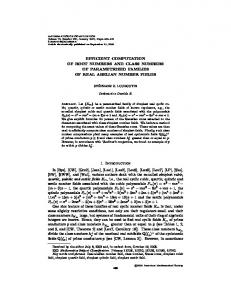
FIG. 2. (Color online) Position and width of the magnon peak for |q| = 0.5 N and |q| = N as a function of the size of the basis. The results appear well converged for a basis size of 46 functions.

4 × 4 × 4 supercell of the Wigner-Seitz cell. Basis functions for other values of R were neglected. The intermediate orthonormal basis described in Appendix B was constructed using a tolerance of tolerance = 10−8 , which produced 220 or 221 basis functions, depending on q; the optimal basis was then obtained from these. The Kohn-Sham susceptibility in the optimal basis representation was computed by interpolating all relevant quantities to a 64 × 64 × 64 fine k mesh.32 Both the “real part” and the “imaginary part” were computed explicitly on a regular frequency mesh with spacing 2 meV in the range [−100,400] meV using adaptive smearing and the Gaussian representation of the δ distribution. The basis set used was of the form described in Eq. (84), namely, the functions {|1,|mz ,|} plus functions of the form |mz × Aαq  for many shells of G vectors. The overlap between {|1,|,|mz } and their projections on the optimal basis subspace was very good, with the “leakage” angle of Appendix B bounded as cos θqi  0.998. In order to assess convergence, computations where performed at |q| = 0, 0.5 N and N with up to 13 shells of G vectors (a maximum of 83 basis functions); it was determined that eight shells (46 basis functions) were sufficient to reach convergence (see Fig. 2). 1. Gap error

ξnk (eV)

5 4 3 2 1 0 -1 -2 -3 -4 -5

|q| = 0.5 ΓN

50

Γ

H

P N

↑

Γ

↓

H

N

Γ

P N

Wannier

FIG. 1. (Color online) Band structure of iron as computed ab initio (full lines) and interpolated using MLWF (dashed line). The interpolation is indistinguishable for all practical purposes from the first-principles calculation for energies between approximately F − 10 eV and F + 30 eV; the Fermi energy is set to zero on the graph.

As discussed in Sec. IV, a gap error h ¯ ω in the magnon spectrum is to be expected due to the difference between (gs) (χ) |mz  and |mz . In order to demonstrate this explicitly, the “imaginary part” of the susceptibility for q = 0 was computed on a regular frequency mesh with spacing 2.5 meV in the range [−28,28] eV using Gaussian adaptive smearing, leaving the “real part” of the susceptibility to be obtained a posteriori from the Kramers-Kronig relations. It is straightforward to demonstrate that the different set of parameters lead to different magnetization densities. For (χ) instance, mz,G=0 can be obtained using the sum rule described in Appendix C; this can be compared to the value obtained from the ground-state calculation,

054305-8

(gs) m = 2.107 N z,G=0

and

(χ) m = 2.163, N z,G=0

(114)

EFFICIENT COMPUTATION OF MAGNON DISPERSIONS . . .

PHYSICAL REVIEW B 85, 054305 (2012)

is linear. According to Eq. (103), the relationship should be

1.0

h ¯ ω = s,  (gs)  (gs)  m z m z s =  (gs)   . mz J

Λ (× 10−2)

0.5 0.0

-0.5

mz (r) , (118)  where  is the gap between minority and majority spins and thus J (r) 

-1.5 5

6

7

8 9 h ¯ ωKK (eV)

10

11

12

s  .

FIG. 3. (Color online) Values of  in iron, artificially made to be a function of the Kramers-Kronig integration bound h ¯ ωKK . The error is zero for h ¯ ωKK  7 eV.

showing that there is about a 3% discrepancy between the two results. In order to gauge the effect of this discrepancy, we define  (gs)  (gs)  ˆ ωKK  m z M q=0 (ω = 0) mz , (¯hωKK ) =  (gs)  (gs)  mz mz 

(115)

where [−¯hωKK ,¯hωKK ] are the bounds used in the KramersKronig integral used to obtain the “real part” of the susceptibility from the “imaginary part.” The dependence on the integration bound h ¯ ωKK is in a sense artificial, as the correct limit would be h ¯ ωKK → ∞, but introducing this dependence (χ) allows the tuning of |mz , which will be quite useful for what follows.  is plotted for iron in Fig. 3, where it can be seen that it is fortuitously very small for h ¯ ωKK  7 eV. The gap error h ¯ ω was also computed for various values of h ¯ ωKK ; its relationship to the corresponding value of  can be seen in Fig. 4. This figure makes it clear that even a modest relative error of a few percent corresponds to a very large gap error, on the magnon energy scale, and that the relationship between the two errors 60 40 h ¯ ωΓ (meV)

(117)

It is straightforward to estimate the value of the slope; neglecting dispersion in the denominator of Eq. (101),

-1.0

-2.0

(116)

h ¯ ωΓ = 1838 × Λ − 0.9 meV Computed points

From Fig. 1,   2 eV, in excellent agreement with the slope of 1.8 eV extracted by linear fitting in Fig. 4. 2. Magnon dispersion

The computed magnon dispersion is shown on Fig. 5 for a basis set containing 46 basis functions. The magnon dispersion is compared to previous experimental33 as well as theoretical2,7,34 results. All theoretical data sets agree very well for |q|  0.4 N; past this point, the dispersion enters the electron-hole continuum, the spectral peaks acquire significant width and there are large variations in the results from the literature. The computed spectrum at |q| = 0.4375 N presents two peaks of roughly equal height; multiple peaks were not observed at other q points. The various theoretical calculations do not agree well with the experimental data of Loong et al.:33 this could be due to the fact that measurements are performed at finite temperature, whereas the computations assume T = 0 K, leading to a sharp Fermi surface. Furthermore, due to the measurement method used, q did not lie in the N direction but varied in the N-H plane. The results presented here suggest the presence of a very shallow maximum in the dispersion, a feature already present in the polarized free-electron gas.35 It is remarkable that our results agree best with those of Halilov et al.,34 which were obtained using an adiabatic method. In order to understand the origin of this good agreement, the adiabatic spectrum can be extracted from the data using an expansion of the form ˆ q, χˆ −1 hω)  −αˆ ∗q + h ¯ ω q (¯

20

(120)

with

0

∂ −1 χˆ (¯hω). (121) h ¯ ω→0 ∂¯ hω q αˆ q describes the stiffness of the ground state as described in ˆ q can be expressed as a Berry curvature.36–38 Appendix D and  Neglecting damping, the magnon frequency is given by ˆ q = lim hω = 0),  αˆ ∗q = −χˆ −1 q (¯

-20 -40 -60 -3

(119)

-2

-1

0 1 Λ (× 10−2)

2

3

χˆ −1 hωq )|mq  = 0, q (¯

FIG. 4. (Color online) Gap error corresponding to various values of  in iron. The gap error is essentially linear with . The line represents a linear fit with a slope of 1.8 eV.

(122)

the adiabatic approximation h ¯ ωqad can then be obtained as the ˆ −1 · αˆ ∗ . The real part of the smallest eigenvalue of the matrix  q q ˆ q was obtained by using a finite difference scheme matrix 

054305-9

BRUNO ROUSSEAU, ASIER EIGUREN, AND AITOR BERGARA

PHYSICAL REVIEW B 85, 054305 (2012)

˚ −1) |q| (A 0.8

1.0

1.2

≥0.4

1.4

Loong et al. (exp.) Karlsson et al. (theory) Buczek et al. (theory) Halilov et al. (theory) this work

0.3

h ¯ ω (meV)

300

200

0.2

100

0

0.25

0.5

0.75

N

|q| (fraction of ΓN distance)

0.4

0.6

0.8

1.0

1.2

≥4.0

1.4

3.0

300

200

2.0

100

0.1

Γ

0.2

400

0 0.0

-Im[χ] (1/eVa03)

0.6

h ¯ ω (meV)

0.4

-Im[χKS] (10−3× 1/eVa30)

0.2

400

˚ −1) |q| (A

1.0

Γ

0.25

0.5

0.75

N

0.0

|q| (fraction of ΓN distance)

(a)

(b)

FIG. 5. (Color online) Magnon dispersion in iron along N. (a) Red (grey) circles represent the position of the maxima in the spectra and the error bars is the full width at half maximum. The colored background represents −Im[χ KS (q,ω)00 ], indicating the presence of the electron-hole continuum. Results from this work are compared to the experimental results of Loong et al.33 as well as to the theoretical results of Karlsson and Aryasetiawan,2 Buczek et al.,7 and Halilov et al.34 (b) Color map representing −Im[χ (q,ω)00 ] in units of 1/eVa03 .

with respect to frequency; the resulting adiabatic frequencies are presented on Fig. 6, along with the dispersion obtained from the dynamic formalism. The work by Halilov et al.34 neglects the Berry curvature contribution:39 in order to obtain a more direct comparison, approximate adiabatic frequencies ˆ q → c1, ˆ with the constant c chosen were also obtained using  so that the frequency would agree with the full adiabatic solution at |q| = N. Figure 6 makes it clear that sharp features are present in the adiabatic spectrum, even when neglecting ˆ q . It is straightforward to show that such strong features due  to αˆ q are absent in the polarized free-electron gas at the level of the LDA; the band structure of iron is far from free electron like, however, and, as pointed out by Halilov et al.,34 there is significant Fermi surface nesting leading to sharp features even in the approximate adiabatic spectrum.

B. Nickel

The ground-state density of fcc nickel within LDA was obtained using a norm conserving pseudopotential with 3d and 4s states as valence, an energy cutoff of 180 Ry and a 26 × 26 × 26 -centered Monkhorst-Pack k mesh. The occupation factors were smeared using the “cold smearing” scheme with a smearing parameter of 1 mRy. The lattice spacing was set to the experimental value of 6.652 a0 . The resulting magnetization was 0.61μB per unit cell, in excellent agreement with tabulated experimental values. Periodic functions were represented in real space on a regular 45 × 45 × 45 grid covering the WignerSeitz cell. The band structure was generated on a 8 × 8 × 8 coarse k mesh, and 26 MLWF were generated by disentangling subspaces containing 44 bands. As can be seen in Fig. 7, the 5 4

300

3

Dynamic frequencies Adiabatic frequencies Adiabatic frequencies, neglecting Ω q

ξnk (eV)

200

2

Halilov et al.

1 0

h ¹ ω (meV)

-1 -2 -3

100

-4 -5

Γ

W K

↑

0 Γ

0.25 0.5 0.75 |q| (fraction of Γ N distance)

L

↓

W

X

Γ

Wannier

N

FIG. 6. (Color online) Adiabatic and approximate adiabatic dispersions, compared to the results from the full calculation and the approximate adiabatic results of Halilov et al.34

FIG. 7. (Color online) Band structure of nickel, as computed ab initio (full lines) and interpolated using MLWF (dashed line). The interpolation is indistinguishable for all practical purposes from the first-principles calculation for energies between approximately F − 10 eV and F + 30 eV; the Fermi energy is set to zero on the graph.

054305-10

EFFICIENT COMPUTATION OF MAGNON DISPERSIONS . . .

PHYSICAL REVIEW B 85, 054305 (2012)

300

Sec. V A), and it was also found that the overlap between {|1,|,|mz } and their projections on the optimal basis subspace was very good, with the “leakage” angle of Appendix B bounded as cos θqi  0.998. In order to assess convergence, computations where performed at |q| = 13/32 N and 29/32 N with up to nine shells of G vectors (a maximum of 42 basis functions); it was determined that six shells (22 basis functions) were sufficient to reach convergence (see Fig. 8).

200

1. Magnon dispersion and spectra

600 500

h ¯ ω (meV)

400

100

|q| = 0.40625 ΓX |q| = 0.90625 ΓX

5

10

15

20 25 basis size

30

35

40

FIG. 8. (Color online) Position and width of the magnon peak in nickel for |q| = 13/32 X and |q| = 29/32 X as a function of the size of the basis. The results appear well converged for a basis size of 22 functions.

Wannier-interpolated band structure is indistinguishable from the one obtained ab initio over an energy range F − 10 eV to F + 30 eV. The Kohn-Sham susceptibility in the optimal basis representation was computed by interpolating all relevant quantities to a 64 × 64 × 64 fine k mesh. Both the “real part” and the “imaginary part” were computed explicitly on a regular frequency mesh with spacing 2 meV in the range [−100,700] meV using adaptive smearing and the Gaussian representation of the δ distribution. The gap error was corrected as described in Sec. IV. The bare product basis functions of Eq. (63) were obtained following the same procedure as for iron (see ˚ −1) |q| (A

˚ −1) |q| (A ≥1.0

0.2 0.4 0.6 0.8 1.0 1.2 1.4 1.6 Mook et al. (exp.) ˘ et al. (theory) S¸as¸ioglu

600

500

0.8

h ¯ ω (meV)

400 0.5

300 200

500 400

h ¯ ω (meV)

Buczek et al. (theory) Halilov et al. (theory) abiabatic frequencies this work

-Im[χKS] (10−3× 1/eVa30)

600

≥2.0

0.2 0.4 0.6 0.8 1.0 1.2 1.4 1.6

1.0

300

-Im[χ] (1/eVa30)

0

The computed magnon dispersion can be seen on Fig. 9. It is well known that LSDA does not properly reproduce the magnon dispersion;3,4 the experimental spectra can be reproduced using LSDA + U 4 or many-body perturbation theory at the level of the RPA.2 Nevertheless, the magnon dispersion computed at the level of LSDA is in qualitative agreement with previous calculations based on the same physical assumptions.4,7 There is excellent quantitative agreement up to the middle of the zone; there remains a spread in the predicted values past 0.5 X, however, where different calculations can differ by up to 100 meV. Despite this spread, the same conclusions already presented by Buczek et al.7 apply. Results by Halilov et al.34 are also presented; their dispersion is seen to be significantly lower than other results, probably a consequence of a systematic error in the computation of the exchange constants.42 Finally, the adiabatic spectrum obtained using the same method as in iron is also presented. The adiabatic frequencies agree well with previous results at small q, but depart drastically from the dynamic results as the spectrum enters the electron-hole continuum, indicating the limitations of this formalism in the region where the spectrum is highly damped. Various spectra for small q are presented in Fig. 10. Although two peaks cannot readily be resolved, the spectra

200

0.2 100 0

100

Γ

0.25

0.5

0.75

|q| (fraction of ΓX distance)

X

0 0.0

Γ

0.25

0.5

0.75

|q| (fraction of ΓX distance)

(a)

X

0.0

(b)

FIG. 9. (Color online) Magnon dispersion in nickel along X. (a) Red (grey) circles represent the position of the maxima in the spectra and the error bars the full width at half maximum. The colored background represents −Im[χ KS (q,ω)00 ], indicating the presence of the electron-hole continuum. The white downward triangles represent the frequencies obtained using the Berry curvature adiabatic formalism. Results from this work are compared to the experimental results of Mook et al.40,41 as well as to the theoretical results of S¸as¸io˘glu et al.,4 Buczek et al.,7 and Halilov et al.34 (b) Color map representing −Im[χ (q,ω)00 ] is in units of 1/eVa03 . 054305-11

BRUNO ROUSSEAU, ASIER EIGUREN, AND AITOR BERGARA

PHYSICAL REVIEW B 85, 054305 (2012)

-Im[χ(q, ω)00] x = 0.0625

ACKNOWLEDGMENTS

x = 0.1250

B.R. is grateful to I. Errea for fruitful discussions. We acknowledge financial support from UPV/EHU (Grant No. IT-366-07).

x = 0.1875

APPENDIX A: EXCHANGE-CORRELATION KERNEL 1.2 1.0 0.8 0.6 0.4 0.2 0.0

x = 0.2500

x = 0.3125

x = 0.3750

The exchange-correlation kernel within the adiabatic LSDA is approximated as14,43 xc xc f↑↓↓↑ (r,r ,t) = f↓↑↑↓ (r,r ,t) ≡ f xc (r,r ,t)

0 100 200 300 400 h ¯ ω (meV)

(A1)

 ∂xc [n,ζ˜ ]  2   δ(r − r )δ(t) ˜ , n(r)ζ (r) ∂ ζ˜ ζ =ζ

|q| = xΓX

FIG. 10. (Color online) Spectra in nickel for |q| = x X for various values of x. All spectra are normalized to have maximum height of 1; all panels have the same dimensions.

(A2)

where xc is the exchange-correlation energy density in the LSDA and n(r) = n↑ (r) + n↓ (r),

(A3) (A4)

are quite broad and asymmetric, suggesting that indeed two branches could be present.

mz (r) = n↑ (r) − n↓ (r), mz (r) ζ (r) = n(r)

VI. CONCLUSION

with nσ (r) the number density of σ spins in the ground state. Given that the spin-dependent exchange-correlation potential is given by

The method presented here allows the efficient computation of magnon dispersions from first principles, avoiding two prominent bottlenecks in the brute force computation of the susceptibility. First, the band structure is Fourier interpolated using MLWF onto a fine k mesh. Second, a well designed basis set that satisfies the acoustic condition is used; this set is significantly smaller than basis sets used previously. Furthermore, the acoustic condition was used to understand the nature of the gap error, and led to a correction scheme consistent with TDDFT that can be generalized to systems where spin-orbit coupling introduces a physical gap in the spectrum. Application of the method to bcc iron yielded a spectrum with sharp features in agreement with previous work by Halilov et al., but differing by up to about 100 meV from results obtained by Karlsson et al. and Buczek et al. As pointed out by Halilov et al., Fermi surface effects are responsible for the sharp features present in the calculation, and it may be that a dense k mesh sampling is required to properly resolve such features. Application of the method to fcc nickel yielded results in good agreement with previous calculations performed at the same level of theory, but a significant 100-meV spread in the predicted values at larger q from one computation to another shows that these calculations can be quite sensitive to computational details. The method can be generalized to other types of electronic excitations, such as plasmons, and to systems where spin is no longer a good quantum number. Given that the method relies on MLWF, which are localized in space, it is ideally suited to study more complex geometries such as surfaces, where describing spatial functions in terms of plane waves is prohibitive. Work is currently under way to study the collective excitations of such systems, where nonbulk geometry and spinorbit coupling have significant effects.

σ (r) = vxc

δ δnσ (r)

(A5)

(A6)

Exc ,

it is straightforward to show that f xc (r,r ,t) = δ(r − r )δ(t)

(r) mz (r)

(A7)

with ↑ ↓ (r) ≡ vxc (r) − vxc (r).

(A8)

The frequency-dependent exchange-correlation kernel can be expressed as 1  iq·(r−r ) xc e fq (r,r ,ω)

q

(A9)

(r)  iG·(r−r ) e mz (r) G

(A10)

1BZ

f xc (r,r ,ω) = with

fqxc (r,r ,ω) =

where a plane-wave representation of the δ distribution has been used. Thus, within the adiabatic LSDA, the kernel has no q or ω dependence. APPENDIX B: BUILDING THE OPTIMAL BASIS

The optimal basis is obtained by first orthogonalizing the overlap matrix24    OqI J = BqI BqJ , (B1) which can be expressed as

054305-12

Oq = VBq · Bq · VB,† q ,

(B2)

EFFICIENT COMPUTATION OF MAGNON DISPERSIONS . . .

where Bq is a diagonal matrix containing the eigenvalues of Oq and VBq is a unitary matrix. For  B    q  LL   tolerance , (B3) Max  B  q II

intermediate orthonormal basis functions {|CqL } are defined as    L B I V B . C =  1 (B4) q q q IL B LL I Any lattice periodic function |g i  can be projected onto this subspace,    Li gqC = CqL g i , (B5)  i    L  C Li g˜ = C g . (B6) q q q L

{|CqL }

The set of functions is not complete, and thus there can i be a difference between |g  and |g˜ qi ; the disparity between the two can be expressed in terms of an angle,  i i   i i  g g˜ q g g˜ q i cos θq =  (B7)     g i |g i  . g i |g i  g˜ qi g˜ qi The departure of cos θqi from 1 is a measure of how much |g i  leaks out of the subspace spanned by {|CqL }. The set of functions {|g i } contains at least the minimal set {|1,|mz ,|} and, optionally, more functions related to plane waves. The “leakage” described above is only of concern for the minimal set, as these functions are necessary to satisfy the acoustic condition and to project the final result onto the G = G = 0 Fourier component. A new orthonormal basis set is defined by first generating orthonormal functions that span ˜ m ˜ ˜ z ,|}; the same subspace as {|1,| more basis functions are added, if need be, using the other functions {|g˜ qi>3 } and the Gram-Schmidt process. The optimal basis is thus finally defined as  i    j  ij  j ij b = g˜ g  |g g , (B8) q

q

q

q

j

j

which can also be explicitly linked to the original, bare product basis,  i    I  Ii B b , b = (B9) q

q

PHYSICAL REVIEW B 85, 054305 (2012)

Consider the integral of this susceptibility over frequency,  ∞ KS d¯hωχ↑↓,↓↑ (r,r ,ω). (C2) I= −∞

It is a simple exercise of complex analysis to show that  ∞ 1 = −iπ, (C3) dx x + y + iη −∞ and thus I = −iπ

q

TI i =

(B10)

(C4)

Since wave functions form a complete set, it is clear that  σ,∗ σ ψnk (r)ψnk (r ) = δ(r − r ). (C5) nk

The integral then becomes I = −iπ δ(r − r ) ×

1BZ 

↑ ↓ × f (ξnk )|ψnk (r)|2 − f (ξnk )|ψnk (r)|2 .

(C6)

nk

The sum above is simply the ground-state magnetization, and thus the sum rule is given by  ∞ d¯hω KS χ↑↓,↓↑ (r,r ,ω) = δ(r − r )mz (r). (C7) i −∞ π The above can be Fourier transformed:  ∞ d¯hω KS i χ↑↓,↓↑ (q,ω)GG = mz,G−G , −∞ π where mz (r) =



eiG·r mz,G .

(C8)

(C9)

G

In particular, for G = G = 0,  ∞ d¯hω KS − (q,ω)00 ] = mz,G=0 . Im[χ↑↓,↓↑ −∞ π

q

 ∗ bqJ i OqJ I .

k n1 ,n2

↑,∗ ↓ ↓,∗ ↑ × ψn1 k (r)ψn2 k+q (r)ψn2 k+q (r )ψn1 k (r ).

(C10)

APPENDIX D: ACOUSTIC CONDITION AND GOLDSTONE’S THEOREM

I

leading to

1BZ  1BZ      

f ξn1 k − f ξn2 k+q

It is well known that, in the absence of spin-orbit coupling, the magnon dispersion for small momentum is of the form

J

h ¯ ωq  D|q|2 , APPENDIX C: SUSCEPTIBILITY SUM RULE

The Kohn-Sham transverse magnetic susceptibility is given by KS χ↑↓,↓↑ (r,r ,ω)

=

1BZ  1BZ   q

k n1 ,n2

    f ξn1 k − f ξn2 k+q h ¯ ω + ξn1 k − ξn2 k+q + iη

↑,∗ ↓ ↓,∗ ↑ × ψn1 k (r)ψn2 k+q (r)ψn2 k+q (r )ψn1 k (r ).

(C1)

(D1)

and thus the magnon energy vanishes as q → 0 (this will be referred to as the acoustic condition). Intuitively, it is quite easy to see why this must be: the ground state of a ferromagnet spontaneously breaks spin rotational symmetry by exhibiting a magnetization even in the absence of an external magnetic field; the magnetization direction is arbitrary, so it must cost no energy to rotate this direction globally, which is precisely what a magnon represents in the limit q → 0. It will be useful to explore this argument in greater detail.

054305-13

BRUNO ROUSSEAU, ASIER EIGUREN, AND AITOR BERGARA 1. Stiffness theorem

Consider a static perturbation Hamiltonian  μB ˆ − (r)δB + (r)]; (D2) ˆ + (r)δB − (r) + m δ Hˆ = dr[m 2 the total free energy in the presence of the perturbation, viewed as a functional of the magnetization, is given by (T = 0 K is assumed for simplicity), ˜ = Hˆ + δ Hˆ m+δm˜ Etot [m + δ m]

PHYSICAL REVIEW B 85, 054305 (2012)

The equilibrium value of the perturbed magnetization minimizes the total energy, i.e.,  ˜  δEtot [m + m] =0  ˜ z (r) δm ˜ δ m=δm  = dr αzz (r,r )δmz (r ), (D13)  ˜  δEtot [m + m] ˜ − (r) δm=δm δm ˜  μB + 1 ∗ δB (r) + =0= (r,r )δm+ (r ), (D14) dr α+− 2 2

(D3)

which becomes, to lowest order, ˜ Etot [m + δ m] μB = Hˆ m+δm˜ + 2



˜ − (r)δB + (r)], ˜ + (r)δB − (r) + δ m dr[δ m

and

 ˜  δEtot [m + m] ˜ (r)  δm

(D4)

+

where Hˆ m = minm=m [|Hˆ |]. ˆ

(D5)

The ground-state free energy, in the absence of the external perturbation, is minimized at the ground-state magnetization; ˜ this implies that we can expand to second order for any δ m, Hˆ m+δm˜ = Hˆ m +

1 2



˜ δ m=δm

μB − 1 δB (r) + =0= 2 2



dr α+− (r,r )δm− (r ).

(D15)

Given the relationship between applied external field and response, we must have ∗ −1 (r,r ) = −χ+− (r,r ,ω = 0), α+−

(D16)

and thus the change in total energy is given by



δEtot ≡ Etot [m + δm] − Etot [m]  μB = drδm− (r)δB + (r). 2

˜ α (r)δ m ˜ β (r ), (D6) dr ααβ (r,r )δ m

dr

where {α} describes the stiffness of the ground state with respect to changes of the magnetization44 and repeated greek indices are summed over. Since spin-orbit coupling is neglected, the ground-state energy must be invariant under rotation of the magnetization about the zˆ axis. Since the change in magnetization is arbitrary, this implies   R−1 αγ (θ )αγ θ (r,r )Rθβ (θ ) = ααβ (r,r )

(D7)

for R(θ ) an arbitrary rotation matrix in the xy plane. This can only be satisfied if ⎡ ⎤ αxx αxy 0 α = ⎣ −αxy αxx 0 ⎦ . (D8) 0 0 αzz



ααβ (r,r ) = αβα (r ,r).

In a ferromagnet, the magnetization breaks spin rotational symmetry spontaneously. Correspondingly, there must be a Goldstone mode, which corresponds to a global rotation of the magnetization and which doesn’t change the energy of the system. Thus assuming the magnetization is of the form m(r) = mz (r)ˆz,

m (r) = m(r) + δm(r),  δθ nα Jα · m(r), δm(r) = i

(D20) (D21)

α

(D10)

for {Jα } the generators of 3D rotations,

which implies ∗ α+− (r ,r) = α+− (r,r ).

(D19)

an arbitrary rotation of this magnetization must leave the energy invariant. In particular, consider an infinitesimal rotation ˆ δθ around axis n:

(D9)

Furthermore, we define α+− (r,r ) = αxx (r,r ) + iαxy (r,r ),

(D18)

2. Global rotation in ferromagnet

Given the definition of the stiffness coefficients, 

(D17)

(D11)

Thus

  1 ˆ ˆ ˜ z (r)δ m ˜ z (r ) H m+δm˜ = H m + dr dr αzz (r,r )δ m 2   1 ˜ + (r)δ m ˜ − (r ). + dr dr α+− (r,r )δ m 2 (D12) 054305-14

⎛

0 Jx = ⎝ 0 0 ⎛ 0 Jy = ⎝ 0 i ⎛ 0 Jz = ⎝ i 0

⎞ 0 i ⎠, 0 ⎞ 0 −i 0 0 ⎠, 0 0 ⎞ −i 0 0 0⎠, 0 0 0 0 −i

(D22)

(D23)

(D24)

EFFICIENT COMPUTATION OF MAGNON DISPERSIONS . . .

leading to

PHYSICAL REVIEW B 85, 054305 (2012)

and the corresponding change in total free energy is given by δm(r) = δθ mz (r)[ny xˆ − nx yˆ ],

(D25)

δEtot =

×

or, equivalently, δm± (r) ≡ δmx (r) ± iδmy (r), = −δθ mz (r)[−ny ± inx ].

(D26) (D27)

The corresponding external field is given by μB δB + (r) = δθ [ny − inx ]



−1 dr χ+− (r,r ,ω = 0)mz (r ),

(D28)

1

 (δθ )2  2 nx + n2y 2 

G. Onida, L. Reining, and A. Rubio, Rev. Mod. Phys. 74, 601 (2002). 2 K. Karlsson and F. Aryasetiawan, Phys. Rev. B 62, 3006 (2000). 3 S. Y. Savrasov, Phys. Rev. Lett. 81, 2570 (1998). 4 E. S¸as¸io˘glu, A. Schindlmayr, C. Friedrich, F. Freimuth, and S. Bl¨ugel, Phys. Rev. B 81, 054434 (2010). 5 P. Buczek, A. Ernst, P. Bruno, and L. M. Sandratskii, Phys. Rev. Lett. 102, 247206 (2009). 6 P. Buczek, A. Ernst, and L. M. Sandratskii, Phys. Rev. Lett. 106, 157204 (2011). 7 P. Buczek, A. Ernst, and L. M. Sandratskii, Phys. Rev. B 84, 174418 (2011). 8 G. D. Mahan, Many-Particle Physics (Kluwer Academic, New York, USA, 2000). 9 J. F. Cooke, Phys. Rev. B 7, 1108 (1973). 10 S. L. Adler, Phys. Rev. 126, 413 (1962). 11 N. Wiser, Phys. Rev. 129, 62 (1963). 12 E. Runge and E. K. U. Gross, Phys. Rev. Lett. 52, 997 (1984). 13 R. van Leeuwen, Phys. Rev. Lett. 80, 1280 (1998). 14 K. Capelle, G. Vignale, and C. A. Ullrich, Phys. Rev. B 81, 125114 (2010). 15 S. Baroni, S. de Gironcoli, A. Dal Corso, and P. Giannozzi, Rev. Mod. Phys. 73, 515 (2001). 16 F. Giustino, M. L. Cohen, and S. G. Louie, Phys. Rev. B 81, 115105 (2010). 17 T. Miyake and F. Aryasetiawan, Phys. Rev. B 61, 7172 (2000). 18 N. Marzari and D. Vanderbilt, Phys. Rev. B 56, 12847 (1997). 19 I. Souza, N. Marzari, and D. Vanderbilt, Phys. Rev. B 65, 035109 (2001). 20 J. R. Yates, X. Wang, D. Vanderbilt, and I. Souza, Phys. Rev. B 75, 195121 (2007). 21 P. Giannozzi, S. Baroni, N. Bonini, M. Calandra, R. Car, C. Cavazzoni, D. Ceresoli, G. L. Chiarotti, M. Cococcioni, I. Dabo, A. D. Corso, S. de Gironcoli, S. Fabris, G. Fratesi, R. Gebauer, U. Gerstmann, C. Gougoussis, A. Kokalj, M. Lazzeri, L. Martin-Samos, N. Marzari, F. Mauri, R. Mazzarello, S. Paolini, A. Pasquarello, L. Paulatto, C. Sbraccia, S. Scandolo, G. Sclauzero, A. P. Seitsonen, A. Smogunov, P. Umari, and R. M. Wentzcovitch, J. Phys. Condens. Matter 21, 395502 (2009).

dr

−1 dr mz (r)χ+− (r,r ,ω = 0)mz (r ). (D29)

Of course, this change of energy must vanish because of Goldstone’s theorem; this is satisfied if  −1 (r,r ,ω = 0)mz (r ) = 0, (D30) dr χ+− which is simply the magnon condition of Eq. (21) at zero frequency. Thus emerges a useful result: the profile of the magnon should be proportional to the ground-state magnetization as q → 0. This also implies that crystal local field effects (CLFE) are essential to satisfy the acoustic condition.

22

A. A. Mostofi, J. R. Yates, Y.-S. Lee, I. Souza, D. Vanderbilt, and N. Marzari, Comput. Phys. Commun. 178, 685 (2008). 23 H. J. Monkhorst and J. D. Pack, Phys. Rev. B 13, 5188 (1976). 24 F. Aryasetiawan and O. Gunnarsson, Phys. Rev. B 49, 16214 (1994). 25 S. Lounis, A. T. Costa, R. B. Muniz, and D. L. Mills, Phys. Rev. B 83, 035109 (2011). 26 I. Garate and A. MacDonald, Phys. Rev. B 79, 064403 (2009). 27 M. Lax, Symmetry Principles in Solid State and Molecular Physics (Wiley, New York, USA, 1974). 28 Given that the functional basis {|BqI } is incomplete, the functions {|g˜ qi } actually represent the projections of {|gqi } onto the functional space spanned by {|BqI }. 29 S. Lounis, A. T. Costa, R. B. Muniz, and D. L. Mills, Phys. Rev. Lett. 105, 187205 (2010). 30 J. P. Perdew and A. Zunger, Phys. Rev. B 23, 5048 (1981). 31 N. Marzari, D. Vanderbilt, A. De Vita, and M. C. Payne, Phys. Rev. Lett. 82, 3296 (1999). 32 As a convergence check, computations performed with a 48 × 48 × 48 fine k mesh for q = i/8N, 1  i  8, yielded essentially the same magnon energies. 33 C. K. Loong, J. M. Carpenter, J. W. Lynn, R. A. Robinson, and H. A. Mook, J. Appl. Phys. 55, 1895 (1984). 34 S. V. Halilov, H. Eschrig, A. Y. Perlov, and P. M. Oppeneer, Phys. Rev. B 58, 293 (1998). 35 D. C. Mattis, Phys. Rev. 151, 278 (1966). 36 Q. Niu and L. Kleinman, Phys. Rev. Lett. 80, 2205 (1998). 37 R. Gebauer and S. Baroni, Phys. Rev. B 61, R6459 (2000). 38 Z. Qian and G. Vignale, Phys. Rev. Lett. 88, 056404 (2002). 39 The computations by Halilov et al. may also suffer from a systematic error; see Ref. 42. 40 J. W. Lynn and H. A. Mook, Phys. Rev. B 23, 198 (1981). 41 H. A. Mook and D. M. Paul, Phys. Rev. Lett. 54, 227 (1985). 42 P. Bruno, Phys. Rev. Lett. 90, 087205 (2003). 43 F. Wang and T. Ziegler, J. Chem. Phys. 121, 12191 (2004). 44 F. G. Gabriele and G. Vignale, Quantum Theory of the Electron Liquid (Cambridge University Press, Cambridge, UK, 2005).

054305-15