ABSTRACT. The decomposition of a monaural audio recording into musically meaningful sound sources constitutes one of the central research topics in music ...
EFFICIENT DATA ADAPTION FOR MUSICAL SOURCE SEPARATION METHODS BASED ON PARAMETRIC MODELS Sebastian Ewert? ?
Meinard M¨uller†
Mark Sandler?
Queen Mary University of London, London, United Kingdom † International Audio Laboratories, Erlangen, Germany
ABSTRACT The decomposition of a monaural audio recording into musically meaningful sound sources constitutes one of the central research topics in music signal processing. In this context, many recent approaches employ parametric models that describe a recording in a highly structured and musically informed way. However, a major drawback of such approaches is that the parameter learning process typically relies on computationally expensive data adaption methods. In this paper, the main idea is to distinguish parameters in which the model is linear explicitly from the remaining parameters. Exploiting the linearity we translate the data adaption problem into a sparse linear least squares problem with box constraints (SLLS-BC), a class of problems for which highly efficient numerical solvers exist. First experiments show that our approach based on modified SLLS-BC methods accelerates the data adaption by a factor of four or more compared to recently proposed methods. Index Terms— Source separation, parametric models, numerical optimization, music processing. 1. INTRODUCTION In recent years, methods for the separation of musically meaningful sound sources from monaural music recordings have been applied to many music processing and analysis tasks. For instance, removing the percussion from a given recording led to significant improvements in a subsequent harmonic analysis [1]. Similarly, many existing query-by-humming systems rely on methods for separating the main melody from a polyphonic music recording [2, 3, 4]. Furthermore, extracting sounds with a similar spectral envelope is a fundamental step in the recognition of instruments in polyphonic recordings [5]. In this context, non-negative matrix factorization (NMF) [6] (or its equivalent probabilistic formulation PLCA [7]) is an often employed technique as it is easy to implement and efficient enough for many applications. However, using a purely statistical approach such as standard NMF often leads to unpredictable separation results. To enforce a musically meaningful structure in the signal model, many authors proposed parametric models which allow for integrating available domain knowledge [8, 9, 10, 11, 12, 13, 14, 15, 16]. For example, such models account for the fact that partials in a harmonic sound are equidistantly spaced (on a linear frequency scale) [8, 14, 11], that the physical amplitude progresses rather smoothly in time for many instruments [9, 15], or that the sound produced by many instruments can be compactly explained using a source-filter model [2, 5, 16]. Overall, integrating domain knowledge typically leads to a significant gain in robustness and accuracy when analyzing real-world music recordings. The International Audio Laboratories Erlangen (AudioLabs) are a joint institution of the University of Erlangen-Nuremberg and Fraunhofer IIS.
After finding a parametric model for a given application, the next challenge is to specify the model parameters in such a way that a given recording is explained accurately. To this end, one typically employs numerical optimization procedures to minimize a distance between the model and the recording. However, since such data adaption methods are typically computationally expensive, parametric models can often not be applied to large datasets. Nevertheless, computational efficiency is not in the focus of many current methods. Indeed, most current approaches apply the same basic strategy to all parameters, although the underlying model often has parameterspecific properties, which could be exploited to accelerate the data adaption step. The main idea of this paper is to distinguish between parameters in which a model is linear from those in which it is non-linear. This way, we can exploit the linearity and employ parameter-specific high-efficiency data adaption methods. In particular, using a recent parametric model as an example, we reformulate the data adaption problem for linear parameters as a sparse linear least squares problem with box constraints (SLLS-BC). This new form enables us to employ two methods based on the interior points and active set paradigms, which were specifically designed for this class of problems and offer a high computational efficiency. We increase the performance of these methods even further by adapting them specifically to the needs of data adaption problems. As shown in our experiments, our proposed methods accelerate the data adaption step by a factor of four or more compared to other recently proposed approaches. The remainder of this paper is organized as follows. In Section 2, we start by describing a typical parametric model, which forms the basis of many current approaches and which serves as an example throughout the paper. In Section 3, we summarize a traditional data adaption strategy and show how the linearity in a model can be exploited using SLLS-BC methods to accelerate the learning process. Furthermore, we discuss two modifications of a standard SLLS-BC method which take additional details of the data adaption problem into account to further increase the overall computational efficiency. In Section 4, we report on systematic experiments illustrating the performance gain over the baseline described in Section 3. Conclusions and prospects on future work are given in Section 5. Further related work is discussed in the respective sections. 2. PARAMETRIC MODELS FOR MUSICAL SOURCE SEPARATION In the context of source separation, parametric models are used to learn and explain how individual sound sources contribute to the spectrogram (or another spectral representation) of a given audio recording. Among the various parametric models proposed in recent years, the Harmonic Temporal Structured Clustering (HTC) ap-
(a)
γp,1
(b)
Intensity
Intensity
γp,3
γp,4 γp,5
500
1000
αp,3 αp,4 αp,5
Intensity
αp,2
γp,2
0
(c)
αp,6 αp,7
γp,6
αp,1 1500
0
1
2
Frequency [Hz]
Time [Sec]
3
4
Freq
uenc y [H
z]
ec] Time [S
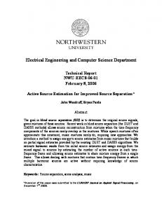
Fig. 1. Variant of the HTC model as presented in [9]. (a) Spectral envelope function Wλn (·, p) for a fixed time frame n, pitch p = 57 (A3, fundamental frequency 220Hz), fundamental frequency parameter τp,n = 0 and some example values for parameter γ. (b) Amplitude progression function Hλ (p, ·) for pitch p = 57, T = 0.5 seconds, and some example values for parameter α. (c) Illustration of the full spectrogram model Yλ combining the submodels shown in (a) and (b).
proach [8, 9] was very successful and forms the basis of many current methods, see for example [11, 12, 14, 15, 17]. The general idea is to use Gaussian functions to represent all parts of the spectrogram model. This way, a harmonic structure can be enforced in frequency direction and a smooth amplitude progression in time direction, see [9, 18] and Fig. 1. In this paper, we employ a slightly simplified version of the HTC model as an illustrative example for parametric models. The following results, however, are general enough to be applicable to the original version of HTC and other parametric models. To describe our model, let X ∈ CM ×N denote the spectrogram and Y = |X| the magnitude spectrogram of a given music recording. Our strategy is to approximate Y by means of a model spectrogram Yλ , where λ denotes a set of free parameters encoding spectral and temporal properties of the recording. To this end, we define Yλ at frequency bin m ∈ [1 : M ] and time frame n ∈ [1 : N ] as X n Yλ (m, n) := Wλ (m, p) · Hλ (p, n), (1) p∈P
where P ⊆ {1, . . . , 127} is a set of MIDI pitches to be considered. The parameter set λ controls the shape of the Gaussian mixture models Wλ and Hλ which capture the spectral envelope and the amplitude progression associated with each MIDI pitch p ∈ P, respectively. More precisely, to describe the frequency and energy distribution of the first L partials of a harmonic sound associated with MIDI pitch p, the parameter set λ contains a time-dependent parameter τ ∈ [−0.5, 0.5]P ×N responsible for fine-tuning the fundamental frequency and a parameter γ ∈ [0, 1]P ×L related to the energy distribution over the L partials, where P := |P|. Using these parameters, we define Wλ as X Wλn (m, p) := γp,` · g(fm − ` · f (p + τp,n )), (2) `∈[1:L]
where fm denotes the center frequency in Hertz associated with the m-th frequency bin of the spectrogram and the function g : R → R≥0 is a suitably chosen Gaussian centered at zero, which is used to describe the shape of a partial in frequency direction. Furthermore, f : R → R≥0 defined by f (p) := 2(p−69)/12 · 440 maps the MIDI pitch to the frequency scale. See Fig. 1(a) for an illustration. ×R Similarly, the set λ contains parameters α ∈ RP controlling ≥0 the amplitude progression over time. More precisely, we define Hλ (p, n) :=
R X r=1
αp,r h(tn − r · T ),
(3)
where tn denotes the center time in seconds associated with time frame n. To allow only smooth amplitude progressions, the zerocentered Gaussian function h : R → R≥0 has a suitably chosen, wide slope. In contrast to Wλ , the position of the individual Gaussians is fixed in Hλ with one of R Gaussians every T seconds, where R := dtN /T e. See Fig. 1(b) for an illustration. Overall, combining the submodels given in Eq. 2 and 3 as in Eq. 1 yields a spectrogram model Yλ suppressing non-harmonic elements in frequency direction and spurious peaks in time direction, see Fig. 1(c) for an illustration. 3. EFFICIENT DATA ADAPTION To explain a given recording using the HTC model, the goal is to find parameters λ = (γ, τ, α) minimizing a distance function between the given spectrogram and the model subject to the non-negativity and domain constraints specified above (e.g. γ ∈ [0, 1]P ×L ). In the following, we use the distance d(γ, τ, α) := kY − Y(γ,τ,α) kF , where k·kF denotes the Frobenius norm. To minimize d, most approaches develop update rules using the same algorithmic framework for all parameters based on some form of gradient descent. For example, approaches based on the HTC model typically compute the partial derivative of d with respect to a single parameter (for our model this means one out of P · (L + N + R) parameters in total). This single dimension gradient descent is often referred to as coordinate descent. To account for non-negativity constraints of the parameters, the step-size for the coordinate descent can be chosen such that the update rules are multiplicative (similar to NMF, see also [6]). For instance, adapting the formulas in [14], the component-wise multiplicative update rule for the parameter γ is: P m,n Y (m, n)g(fm − ` · f (p + τp,n ))Hλ (p, n) . γp,` ← γp,` · P m,n Yλ (m, n)g(fm − ` · f (p + τp,n ))Hλ (p, n) (4) While using an iterative single-parameter update strategy based on the same optimization framework typically leads to easy-toimplement and uniform update rules, it is often computationally expensive. In particular, such methods do not exploit specific properties for the parameters (for example linearity of the spectrogram model), which limits the overall computational efficiency. As a consequence, such methods often require a high number of iterations to converge. This is particularly problematic for update rules as the one given in Eq. 4, as here several computationally expensive Gaussian functions have to be evaluated in each iteration. For a more detailed discussion of the limitations of coordinate descent methods, see also [19, Ch.9].
3.1. Reformulation as an SLLS-BC Problem In order to accelerate the data adaption process, we exploit the linearity of the model for some parameters explicitly using parameterspecific methods instead of using the same algorithmic framework for all parameter. In addition, we update whole parameter groups at the same time instead of optimizing the individual parameters one after another. Using again the parameter γ as an example, we write Yλ as: Yλ (m, n) =
P X X
� � γp,` · g(fm − ` · f (p + τp,n ))Hλ (p, n) .
p=1 `∈[1:L]
(5) In this form, it is straightforward to see that Yλ is linear in γ, i.e. Y(a·γ+b·˜γ ,τ,α) = a·Y(γ,τ,α) +b·Y(˜γ ,τ,α) for a, b ∈ R. Similarly, Yλ is also linear in the amplitude parameters α. To exploit this linearity, we reformulate our parameter estimation problem as follows. First, we define a vector Y˜ ∈ RM ·N by Y˜ ((n − 1)M + m) := Y (m, n), i.e. we simply regard the spectrogram matrix Y as a vector Y˜ by stacking all columns of Y on top of each other. Similarly, fixing τ and α, we define a matrix Aτ,α ∈ R(M ·N )×(P ·L) by Aτ,α ((n − 1)M + m, (p − 1)L + `) :=
(6)
g(fm − ` · f (p + τp,n ))Hλ (p, n) and a vector γ˜ ∈ RP ·L by γ˜ ((p − 1)L + `) := γp,` . As a result it can easily be shown that: d(γ, τ, α) = kY − Y(γ,τ,α) kF = kY˜ − Aτ,α γ˜ k2 .
(7)
With this minor reformulation of our distance function, we have the original problem reduced to a standard linear least squares (LLS) problem, for which many well-studied approaches exist. However, we have to take some additional considerations into account. On the one hand, we require methods respecting the domain constraints for our parameters (e.g. γ ∈ [0, 1]P ×L ). In numerical optimization such constraints are more commonly referred to as bound constraints. On the other hand, the system of linear equations described by Aτ,α is very large. More precisely, Aτ,α as defined in Eq. 6 has a memory requirement of P · L the size of the given spectrogram Y . On the positive side, Aτ,α has additional structure that can be exploited. In particular, comparing Eq. 5 and Eq. 6 we see that column (p−1)L+` of Aτ,α contains only the part of our model spectrogram Yλ that can be scaled using the parameter γp,` . This part only corresponds to a single partial in the entire spectrogram model (the `-th partial in the spectral envelope for pitch p). Therefore, the spectrogram model is only affected in a small area around the center frequency of that partial and hence most entries in each column of Aτ,α are close to zero (in our experiments, typically more than 98% of all entries in Aτ,α were smaller than 10−9 ). By simply thresholding Aτ,α we can store it using sparse matrix data structures and thus significantly reduce the memory requirements. As long as the thresholding is applied carefully the resulting model will not be significantly effected (in our experiments we set every entry in Aτ,α below 10−9 to zero). Overall, our parameter estimation problem can now be considered as a sparse linear least squares problem with bound constraints (SLLSBC) [20]. 3.2. Solving the SLLS-BC Problem In optimization theory, SLLS-BC problems are often considered as a subclass of more generals problems, in particular quadratic and nonlinear programming problems. The majority of these more general
methods are not applicable in our case as they often do not preserve the sparse structure of Aτ,α . However, there are a few methods specific to our problem, see [20] for a detailed discussion. Most of these are based either on the active set (AS) or the interior points (IP) paradigm. The ideas behind both are quite straightforward. Active set methods exploit that solving a linear least squares problem is very efficient as long as there are no constraints to consider, such as our bound constraints. Therefore, AS methods start by solving the unconstrained LLS problem. Given that no constraints are violated we already have our final solution, for example if all entries of the solution vector γ˜ are already between 0 and 1. Otherwise, an algorithm is employed to estimate the so called active set, which encodes the current believe which entries in the final solution vector will be affected by the constraints. Note that in general the active set is not identical to the set of entries violating constraints in the unconstrained solution, see [19] for details. Then the unconstrained LLS problem is solved again with all entries in the active set considered as constant setting them either to the lower or the higher bound. Based on this new solution the active set is reestimated by adding or removing some entries. This process is repeated until the correct active set and the final solution are found, see also [19]. Approaches based on interior point techniques are essentially Newton-type gradient descent methods, i.e. they try to identify a local minimum of our distance function by finding positions where its gradient vanishes. In contrast to active set methods, bound constraints are considered by interior point methods from the start in the form of so called barriers. Barriers constitute additional terms added to the function to be minimized, which penalize violations of constraints in a soft way. After each gradient descent step the influence of the penalty terms is varied in such a way that the method actually converges to the original minimum of d we are looking for. For more details, see for example [19]. In the following, we consider the active set (AS) and the interior points (IP) methods presented in [20]1 . Both were specifically designed for SLLS-BC problems and, as actual solvers, both identify the global minimum of the convex SLLS-BC problem, see [20] for more details. 3.3. Fine-Tuning the Active Set Method Next, we show how the active set method can be adjusted to our specific needs to further raise its computational efficiency. To this end, we exploit that the parameters γ, τ , and α are updated iteratively, i.e. after updating γ, τ , and α, parameter γ is updated again, and so on. The active set method presented in [20] , however, does not exploit this situation as every information about the last iteration is discarded. This is relevant for two steps in the algorithm as we explain next using again parameter γ as an example. First, [20] proposes the use of so called direct methods (Cholesky factorization) to solve the intermediate unconstrained LLS problems as described in the last section. Here, the idea is to factorize the matrix Aτ,α in such a way that the LLS problem can easily be solved, see [19] for more details. This strategy, however, does not exploit the fact that the solution for γ found in the last iteration is actually a good starting point for the current iteration and probably only needs little correction. Therefore, we replace the Cholesky factorization by a method based on Preconditioned Conjugate Gradients (PCG), which can be considered as one of the fastest non-direct solvers, see [19]. As a main advantage PCG allows us to employ the parameter values computed in the last iteration as a starting point, which PCG only needs to refine in the current iteration. Such a strategy is often computationally 1 A Matlab implementation of these approaches is available at http:// www.math.liu.se/˜milun/sls/.
Bach (102s) Chop (311s) Beet (541s) 10−2 10−6 10−2 10−6 10−2 10−6 Base 80s 2099s 253s 6952s 431s 38278s (54) (1426) (46) (1264) (66) (5902) AS 25s 177s 117s 911s 163s 1283s (3) (21) (4) (29) (4) (31) IP 21s 153s 86s 641s 106s 997s (3) (21) (4) (29) (4) (31) AS++ 19s 137s 84s 611s 121s 939s (3) (21) (4) (29) (4) (31)
Table 1. Experimental results for three recordings (Bach, Chop, and Beet) and two convergence levels (ε = 10−2 and ε = 10−6 ).
less expensive than computing a full matrix factorization using direct solvers, even if the matrix is very sparse. A second type of information discarded in [20] between iterations is the choice of the active set. In particular, the active set is always initialized as an empty set, although the active set often does not change across iterations. Therefore, it is a natural idea to reuse the active set we found in the last iteration to initialize the active set in the current iteration. This way, we can often reduce the computational costs of our constrained problem to those of an unconstrained problem.
4. EXPERIMENTS In this section, we report on systematically conducted experiments to illustrate the potential performance gain resulting from our proposed methods. Instead of testing our approach only on short sound snippets in the range of 5 to 20 seconds as done in many other source separation approaches, we use full-length music recordings. Exemplarily, we employ recordings of the first movement of three piano pieces taken from the Saarland Music Database (SMD) [21]: Bach’s Prelude No. 6 BWV 875 (length: 102 seconds), Chopin’s Impromptu No. 4 Op. 66 (length: 311 seconds), and Beethoven’s “The Tempest” Op. 31 No. 2 (length: 541 seconds), which we denote by Bach, Chop, and Beet, respectively. We use single channel versions of these recordings with a sampling rate of 22050 Hz. For our experiments, we employ the HTC model as described in Section 2 to approximate the magnitude spectrogram for each recording. The spectrogram is computed using half-overlapped 93ms Hann windows. Furthermore, we set P = {21, . . . , 108}, i.e. we use the full range of MIDI pitches available on a grand piano. To adapt the model to a given recording, we use the various procedures as discussed in Section 3. As a baseline, we employ the method proposed in [14], which employs a coordinate descent method for all parameters γ, α, and τ . Exploiting the linearity of our HTC model for some parameters, our proposed methods keep the update for τ but replace the ones for γ and α with the interior points (IP) and active set (AS) methods presented in Section 3, respectively. In this context, the modified active set method is referred to as AS++ in the following. For all methods, τ is initialized with 0 while γ and α are initialized using random values between zero and one. To allow for a fair comparison, all methods use the same initial values. All methods were implemented in Matlab 2012b and the experiments were conducted on an Intel Core i5-3570K processor with Windows 7. To indicate the computational performance of a method, we measure the time and number of iterations necessary to reach convergence. To this end, we consider a method as converged after k
iterations if conv(k) :=
d(γk , τk , αk ) − d(γk−1 , τk−1 , αk−1 ) ≤ε d(γk , τk , αk )
for a convergence level ε > 0, where γk , τk , and αk denote the HTC parameters after k update iterations. The time in seconds and number of iterations necessary to reach the convergence levels ε = 10−2 and ε = 10−6 are given in Table 1 for all three recordings. Overall, we can observe that the baseline method requires significantly longer to converge compared to the three proposed methods. For example, using ε = 10−2 , the method AS++ converges after 19 seconds for the Bach example, while the baseline method requires 80 seconds (more than four times slower). This difference in performance is even more obvious for very small values of ε. For example, using ε = 10−6 , the baseline runs roughly 15 times longer than AS++ for the Bach example and roughly 40 times longer for the Beet example. Furthermore, the proposed methods require significantly less iterations to reach a given convergence level. For example, using ε = 10−2 , all three proposed methods converge after 3 iterations while the baseline requires 54 iterations for the Bach example (recall that the three proposed methods compute the same result and hence require the same number of iterations). Additionally, we see that while a single iteration using the baseline method takes significantly less time (80s / 54 = 1.48s per iteration) compared to the proposed methods (19s / 3 = 6.33s per iteration for AS++), the reduction of the distance d is much more effective using the proposed methods and hence they converge significantly faster. Moreover, it should be mentioned that after reaching a given convergence level ε, the absolute distance d(γ, τ, α) was for all three examples lower using the proposed methods compared to the baseline approach. The two extensions presented in Section 3.3 and used in the method AS++ further reduce the time to converge for AS by 23% to 33%. Here, both extensions help to exploit that the last iteration gives valueable information for the current iteration. Comparing IP and AS++, we see no significant differences. However, the simpler implementation of the active set method might be an additional benefit. 5. CONCLUSION In this paper, we presented novel methods to accelerate the data adaption step in parametric models for musical source separation. The idea was to exploit that many parametric models are linear in some parameters and non-linear in others. Treating both groups of parameters individually allowed us to employ highly optimized, problem-specific numerical optimization methods for the linear parameters to solve the data adaption problem efficiently. As indicated by our experiments, the time required for the data adaption step in a source separation application can be reduced by a factor of four or more using our proposed methods compared to a recently presented baseline method. While we focused in this paper on parameters in which our example model is linear, we will explore in the future how the data adaption can be accelerated for parameters where linearity is not given. As discussed in [14], the distance function d is often highly non-convex for non-linear parameters, which makes it difficult to solve the minimization problem efficiently without ending up in a random local minimum of d. For parameters such as our τ it seems promising to discretize the parameter domain such that we only need to pick from a finite set of possible parameter values. Such problems can be solved for example using sparse coding techniques [22].
6. REFERENCES [1] Yushi Ueda, Yuuki Uchiyama, Takuya Nishimoto, Nobutaka Ono, and Shigeki Sagayama, “HMM-based approach for automatic chord detection using refined acoustic features,” in Proceedings of the IEEE International Conference on Acoustics, Speech and Signal Processing (ICASSP), Dallas, USA, 2010, pp. 5518–5521. [2] Jean-Louis Durrieu, Ga¨el Richard, Bertrand David, and C´edric F´evotte, “Source/filter model for unsupervised main melody extraction from polyphonic audio signals,” IEEE Transactions on Audio, Speech and Language Processing, vol. 18, no. 3, pp. 564–575, 2010.
[13] Romain Hennequin, Bertrand David, and Roland Badeau, “Score informed audio source separation using a parametric model of non-negative spectrogram,” in Proceedings of the IEEE International Conference on Acoustics, Speech and Signal Processing (ICASSP), Prague, Czech Republic, 2011, pp. 45–48. [14] Romain Hennequin, Roland Badeau, and Bertrand David, “Time-dependent parametric and harmonic templates in nonnegative matrix factorization,” in Proceedings of the International Conference on Digital Audio Effects (DAFx), Graz, Austria, 2010, pp. 246–253.
[3] Justin Salamon and Emilia G´omez, “Melody extraction from polyphonic music signals using pitch contour characteristics,” IEEE Transactions on Audio, Speech, and Language Processing, vol. 20, no. 6, pp. 1759–1770, 2012.
[15] Jun Wu, Emmanuel Vincent, Stanislaw Andrzej Raczynski, Takuya Nishimoto, Nobutaka Ono, and Shigeki Sagayama, “Multipitch estimation by joint modeling of harmonic and transient sounds,” in Proceedings of the IEEE International Conference on Acoustics, Speech, and Signal Processing (ICASSP), Prague, Czech Republic, 2011, pp. 25–28.
[4] Nattha Phiwma and Parinya Sanguansat, “A music information system based on improved melody contour extraction,” in Proceedings of the IEEE International Conference on Signal Acquisition and Processing (ICSAP), Bangalore, India, 2010, pp. 85–89.
[16] Pablo Sprechmann, Pablo Cancela, and Guillermo Sapiro, “Gaussian mixture models for score-informed instrument separation,” in IEEE International Conference on Acoustics, Speech and Signal Processing (ICASSP), Kyoto, Japan, 2012, pp. 49–52.
[5] Toni Heittola, Anssi P. Klapuri, and Tuomas Virtanen, “Musical instrument recognition in polyphonic audio using sourcefilter model for sound separation,” in Proceedings of the International Society for Music Information Retrieval Conference (ISMIR), Kobe, Japan, 2009, pp. 327–332.
[17] Katsutoshi Itoyama, Masataka Goto, Kazunori Komatani, Tetsuya Ogata, and Hiroshi G. Okuno, “Integration and adaptation of harmonic and inharmonic models for separating polyphonic musical signals,” in Proceedings of the IEEE International Conference on Acoustics, Speech and Signal Processing (ICASSP), Hawaii, USA, 2007, pp. I–57–I–60.
[6] Daniel D. Lee and H. Sebastian Seung, “Algorithms for nonnegative matrix factorization,” in Proceedings of the Neural Information Processing Systems (NIPS), Denver, CO, USA, 2000, pp. 556–562. [7] Madhusudana Shashanka, Bhiksha Raj, and Paris Smaragdis, “Probabilistic latent variable models as nonnegative factorizations (article id 947438),” Computational Intelligence and Neuroscience, vol. 2008. [8] Masataka Goto, “A real-time music-scene-description system: Predominant-F0 estimation for detecting melody and bass lines in real-world audio signals,” Speech Communication (ISCA Journal), vol. 43, no. 4, pp. 311–329, 2004. [9] Hirokazu Kameoka, Takuya Nishimoto, and Shigeki Sagayama, “A multipitch analyzer based on harmonic temporal structured clustering,” IEEE Transactions on Audio, Speech and Language Processing, vol. 15, no. 3, pp. 982–994, 2007. [10] Katsutoshi Itoyama, Masataka Goto, Kazunori Komatani, Tetsuya Ogata, and Hiroshi G. Okuno, “Instrument equalizer for query-by-example retrieval: Improving sound source separation based on integrated harmonic and inharmonic models,” in Proceedings of the International Conference for Music Information Retrieval (ISMIR), Philadelphia, USA, 2008, pp. 133– 138. [11] Sebastian Ewert and Meinard M¨uller, “Estimating note intensities in music recordings,” in Proceedings of the IEEE International Conference on Acoustics, Speech, and Signal Processing (ICASSP), Prague, Czech Republic, 2011, pp. 385–388. [12] Sebastian Ewert and Meinard M¨uller, “Score-informed voice separation for piano recordings,” in Proceedings of the International Society for Music Information Retrieval Conference (ISMIR), Miami, USA, 2011, pp. 245–250.
[18] Sebastian Ewert and Meinard M¨uller, “Score-informed source separation for music signals,” in Multimodal Music Processing, Meinard M¨uller, Masataka Goto, and Markus Schedl, Eds., vol. 3 of Dagstuhl Follow-Ups, pp. 73–94. Schloss Dagstuhl–Leibniz-Zentrum fuer Informatik, Dagstuhl, Germany, 2012. [19] Jorge Nocedal and Stephen J. Wright, Numerical Optimization, Springer (Springer Series in Operations Research and Financial Engineering), 2006. [20] Mikael Adlers, Sparse Least Squares Problems with Box Constraints, Ph.D. thesis, Link¨opings Universitet, Sweden, 1998. [21] Meinard M¨uller, Verena Konz, Wolfgang Bogler, and Vlora Arifi-M¨uller, “Saarland music data (SMD),” in Proceedings of the International Society for Music Information Retrieval Conference (ISMIR): Late Breaking session, 2011. [22] Nicolae Cleju, Maria G. Jafari, and Mark D. Plumbley, “Analysis-based sparse reconstruction with synthesis-based solvers,” in IEEE International Conference on Acoustics, Speech and Signal Processing (ICASSP), Kyoto, Japan, 2012, pp. 5401–5404.